Towards SMT Model Checking of Array-based Systems

Towards SMT Model Checking of Array-based Systems Silvio Ghilardi1 , Enrica Nicolini2 , Silvio Ranise1,2 , and Daniele Zucchelli1 1

Dipartimento di Informatica, Universit` a degli Studi di Milano (Italia) 2 LORIA & INRIA-Lorraine, Nancy (France)

Abstract. We introduce the notion of array-based system as a suitable abstraction of infinite state systems such as broadcast protocols or sorting programs. By using a class of quantified-first order formulae to symbolically represent array-based systems, we propose methods to check safety (invariance) and liveness (recurrence) properties on top of Satisfiability Modulo Theories solvers. We find hypotheses under which the verification procedures for such properties can be fully mechanized.

1

Introduction

Model checking of infinite-state systems manipulating arrays – e.g., broadcast protocols, lossy channel systems, or sorting programs – is a hot topic in verification. The key problem is to verify the correctness of such systems regardless of the number of elements (processes, data, or integers) stored in the array, called uniform verification problem. In this paper, we propose array-based systems as a suitable abstraction of broadcast protocols, lossy channel systems, or, more in general, programs manipulating arrays (Section 3). The notion of array-based system is parametric with respect to a theory of indexes (which, for parametrized systems, specifies the topology of processes) and a theory of elements (which, again for parametrized systems, specifies the data manipulated by the system). Then (Section 3.1), we show how states and transitions of a large class of array-based systems can be symbolically represented by a class of quantified first-order formulae whose satisfiability problem is decidable under reasonable hypotheses on the theories of indexes and elements (Section 4). We also sketch how to extend the lazy Satisfiability Modulo Theories (SMT) techniques [16] by a suitable instantiation strategy to handle universally quantified variables (over indexes) so as to implement the satisfiability procedure for the class of quantified formulae under consideration (Figure 2). The capability to handle a (limited form) of universal quantification is crucial to reduce entailment between formulae representing states to satisfiability of a formula in the class of quantified formulae previously defined. This observation together with closure under pre-image computation of the kind of formulae representing unsafe states allows us to implement a backward reachability procedure (see, e.g., [12], or also [15] for a declarative approach) for checking safety properties of array-based systems (Section 5). In general, the procedure may not terminate;

c

SpringerVerlag 2008

but, under some additional assumptions on the theory of elements, we are able to prove termination by revisiting the notion of configuration (see, e.g., [1]) in first-order model-theory (Section 5.2). Finally (Section 6), we show the flexibility of our approach by studying the problem of checking the class of liveness properties called recurrences [13]. We devise deductive methods to check such properties based on the synthesis of so-called progress conditions at quantifier free level and we show how to fully mechanize our technique under the same hypotheses for the termination of the backward reachability procedure. For space reasons, we did not include proofs; for the same reason, although our framework covers all examples discussed in [2,3] (and more), only one running example is discussed. For both proofs and examples, the reader is referred to the Technical Report [10].

2

Formal Preliminaries

We assume the usual first-order syntactic notions of signature, term, formula, quantifier free formula, and so on; equality is always included in our signatures. If x is a finite set of variables and Σ is a signature, by a Σ(x)-term, -formula, etc. we mean a term, formula, etc. in which at most the x occur free (notations like t(x), ϕ(x) emphasize the fact that the term t or the formula ϕ in in fact a Σ(x)-term or a Σ(x)-formula, respectively). The notions of interpretation, satisfiability, validity, and logical consequence are also the standard ones; when we speak about satisfiability (resp. validity) of a formula containing free variables, we mean satisfiability of its existential (resp. universal) closure. If M = (M, I) is a Σ-structure, a Σ-substructure of M is a Σ-structure having as domain a subset of M which is closed under the operations of Σ (in a Σ-substructure, moreover, the interpretation of the symbols of Σ is given by restriction). The Σstructure generated by a subset X of M (which is not assumed now to be closed under the Σ-operations) is the smallest Σ-substructure of M whose domain contains X and, if this Σ-substructure coincides with the whole M, we say that X generates M. A Σ-embedding (or, simply, an embedding) between two Σ-structures M = (M, I) and N = (N, J ) is any mapping µ : M −→ N among the corresponding support sets which is an isomorphism between M and the Σ-substructure of N whose underlying domain is the image of µ (thus, in particular, for µ to be an embedding, the image of µ must be closed under the Σ-operations). A class C of structures is closed under substructures iff whenever M ∈ C and N is (isomorphic to) a substructure of M, then N ∈ C. Contrary to previous papers of ours, we prefer to have here a more liberal notion of a theory, so we identify a theory T with a pair (Σ, C), where Σ is a signature and C is a class of Σ-structures (the structures in C are called the models of T ). The notion of T -satisfiability of ϕ means the satisfiability of ϕ in a Σ-structure from C; similarly, T -validity of a sentence ϕ (noted T |= ϕ) means the truth of ϕ in all M ∈ C. The Satisfiability Modulo Theory T , SMT(T ), problem amounts to establish the T -satisfiability of an arbitrary first-order formula (hence possibly containing quantifiers), w.r.t. some background theory T .

A theory solver for the theory T (T -solver) is any procedure capable of establishing whether any given finite conjunction of literals is T -satisfiable or not. The so-called lazy approach to solve SMT(T ) problems for quantifier-free formulae consists of integrating a Boolean enumerator (usually based on a refinement of the DPLL algorithm) with a T -solver (see [14,16] for an overview). Hence, by assuming the existence of a T -solver, it is always possible to build a (lazy SMT) solver capable of checking the T -satisfiability of arbitrary Boolean combinations of atoms in T (or, equivalently, quantifier-free formulae). For efficiency, a T -solver is required to provide a more refined interface, such as returning a subset of a T -unsatisfiable input set of literals which is still T -unsatisfiable, called conflict set (again see [16] for details). We say that T admits quantifier elimination iff for every formula ϕ(x) one can compute a quantifier-free formula ϕ0 (x) which is T -equivalent to it (i.e. such that T |= ∀x(ϕ(x) ↔ ϕ0 (x))). Linear Arithmetics, Real Arithmetics, acyclic lists, and enumerated datatype theories (see below) admit elimination of quantifiers. A theory T = (Σ, C) is said to be locally finite iff Σ is finite and, for every finite set of variables x, there are finitely many Σ(x)-terms t1 , . . . , tkx such that for every further Σ(x)-term u, we have that T |= u = ti (for some i ∈ {1, . . . , kx }). The terms t1 , . . . , tkx are called Σ(x)-representative terms; if they are effectively computable from x (and ti is computable from u), then T is said to be effectively locally finite (in the following, when we say ‘locally finite’, we in fact always mean ‘effectively locally finite’). If Σ is finite and does not contain any function symbol (i.e. Σ is a purely relational signature), then any Σ-theory is effectively locally finite; other effectively locally finite theories are Boolean algebras and Linear Arithmetic modulo a fixed integer. Let Σ be a finite signature; an enumerated datatype theory in Σ is a theory whose class of models contains only a single finite Σ-structure M = (M, I); we require M to have the additional property that for every m ∈ M there is a constant c ∈ Σ such that cI = m. It is easy to see that an enumerated datatype theory admits quantifier elimination (since ∃x ϕ(x) is T -equivalent to ϕ(c1 ) ∨ · · · ∨ ϕ(cn ), where c1 , ..., cn are interpreted as the finitely many elements of the enumerated datatype) and is effectively locally finite. In the following, it is more natural to adopt a many-sorted language. All notions introduced above (such as term, formula, structure, and satisfiability) can be easily adapted to many-sorted logic, see e.g. Chapter XX of [8].

3

Array-based Systems and their Symbolic Representation

We develop a framework to state and solve model checking problems for safety and liveness of a particular class of infinite state systems by using deductive (more precisely, SMT) techniques. We focus on the class of systems whose state can be described by a finite collections of arrays, which we call array-based systems. As an example, consider parameterized systems, i.e. systems consisting of an arbitrary number of identical finite-state processes organized in a linear

array: a state a of such a parameterized system can be seen as a state of an array-based system (in the formal sense of Definitions 3.2 and 3.3 below), where the indexes of the domain of the function assigned to the state variable a are the identifiers of the processes and the elements of a are the data describing one of the finitely many states of each process. Array-based Systems. To develop our formal model, we introduce three theories. We use two mono-sorted theories TI = (ΣI , CI ) (of indexes) and TE = (ΣE , CE ) (of elements), whose only sort symbol are called INDEX and ELEM, respectively. TI specifies the ‘topology’ of the processes, e.g., in the case of parameterized systems informally discussed above, ΣI contains only the equality symbol ‘=’ and CI is the class of all finite sets. Other interesting examples of TI can be obtained by taking ΣI to contain a binary predicate symbol R (besides =) and CI to be the class of structures where R is interpreted as a total order, a graph, a forest, etc. For parameterized systems with finite-state processes, TE can be the theory of an enumerated datatype. For the larger class of parameterized systems (e.g., the one considered in [2,3]) admitting integer (or real) variables local to each process, TE can be the theory whose class of models consists of a single structure (like real numbers under addition and/or ordering). Notice that in concrete applications, TE has a single model (e.g. an enumerate datatype, or the structure of real/natural numbers under suitable operations and relations), whereas TI has many models (e.g. it has as models all sets, all finite sets, all graphs, all finite graphs, etc.). The technical hypotheses we shall need in Sections 4 and 5 on TI and TE are fixed in the following: Definition 3.1. An index theory TI = (ΣI , CI ) is a mono-sorted theory (let us call INDEX its sort) which is locally finite, closed under substructures and whose quantifier free fragment is decidable for TI -satisfiability. An element theory TE = (ΣE , CE ) is a mono-sorted theory (let us call ELEM its sort) which admits quantifier elimination and whose quantifier free fragment is decidable for TE -satisfiability. One may wonder how restrictive are the assumptions of the above definition: it turns out that they are very light (for instance, they do not rule out any of the examples considered in [2,3]). In fact, quantifier elimination holds for common datatype theories (integers, reals, enumerated datatypes, etc.) and the hypotheses on index theory are satisfied by most process ‘topologies’.3 The third theory AE I = (Σ, C) we need is obtained by combining an index theory TI and an element theory TE as follows. First, AE I has three sort symbols: INDEX, ELEM, and ARRAY; the signature Σ contains all the symbols in the disjoint union ΣI ∪ ΣE and a further binary function symbol apply of sort ARRAY × INDEX −→ ELEM. (In the following, we abbreviate apply(a, i) with a[i], for a term of sort ARRAY and i term of sort INDEX.) Second, a three-sorted structure M = (INDEXM , ELEMM , ARRAYM , I) is in the class C iff ARRAYM is the set 3

They typically fail when processes are arranged in a ring (e.g. in the ‘dining philosophers’ example): rings require a unary function symbol to be formalized and the bijectivity constraint to be imposed is insufficient to make the theory locally finite.

of (total) functions from INDEXM to ELEMM , the function symbol apply is interpreted as function application (i.e. as the standard reading operation for arrays), and (INDEXM , I|ΣI ), (ELEMM , I|ΣE ) are models of TI and TE , respectively – here I|ΣI , I|ΣE are the restriction of I to the symbols of ΣI , ΣE . (In the following, we use the notations MI and ME for (INDEXM , I|ΣI ) and (ELEMM , I|ΣE ), reM spectively.) If the model M of AE is a finite set, then M I is such that INDEX is called a finite index model. For the remaining part of the paper, we fix an index theory TI = (ΣI , CI ) and an element theory, TE = (ΣE , CE ) (we also let AE I = (Σ, C) be the corresponding combined theory). Once the theories constraining indexes and elements are fixed, we need the notions of state, initial state and state transition to complete our picture. In a symbolic setting, these are provided by the following definitions: Definition 3.2. An array-based (transition) system (for (TI , TE )) is a triple S = (a, I, τ ) where: – a is a tuple of variables of sort ARRAY (these are the state variables); – I(a) is a Σ(a)-formula (this is the initial state formula); – τ (a, a0 ) is a Σ(a, a0 )-formula – here a0 is a renamed copy of the tuple a (this is the transition formula). Definition 3.3. Let S = (a, I, τ ) be an array-based transition system. Given a model M of the combined theory AE I , an M-state (or, simply, a state) of S is an assignment mapping the state variables a to total functions s from the domain of MI to the domain of ME . A run of the array-based system is a (possibly infinite) sequence s0 , s1 , ... of states such that4 M |= I(s0 ) and M |= τ (sk , sk+1 ) for k ≥ 0. For simplicity, below, we assume that the tuple of array state variables a is a single variable a: all definitions and results of the paper can be easily generalized to the case of finitely many array variables and to the case of multi-sorted TI , TE (see [10] for a discussion on these topics). 3.1

Symbolic Representation of States and Transitions

The next step is to identify suitable syntactic restrictions for the formulae I, τ appearing in the definition of an array-based system. Preliminarily, we introduce some notational conventions that alleviate the burden of writing and understanding the various formulae for states and transitions: d, e, . . . range over variables of sort ELEM, a, b . . . over variables of sort ARRAY, i, j, k, . . . over variables of sort INDEX, and α, β, . . . over variables of either sort ELEM or sort INDEX. An underlined variable name abbreviates a tuple of variables of unspecified (but finite) length; by subscripting with an integer an underlined variable name, we indicate the corresponding component of the tuple (e.g., i may abbreviate i1 , . . . , in 4

Notations like M |= I(s0 ) means that the formula I(a) is true in M under the assignment mapping the a’s to the s0 ’s.

and ik indicates ik , for 1 ≤ k ≤ n). We also use a[i] to abbreviate the tuple of terms a[i1 ],V . . . , a[in ]. If j and i are tuples with the same length n, then n i = j abbreviates k=1 (ik = j k ). Possibly sub/super-scripted expressions of the forms φ(α), ψ(α), . . . (with sub-/super-scripts) always denote quantifier-free (ΣI ∪ ΣE )-formulae in which at most the variables α occur (notice in particular that no array variable and no apply constructor a[i] can occur here). Also, φ(α, t/β) (or simply φ(α, t)) abbreviates the substitution of the terms t for the variables β (now apply constructors may appear in t). Thus, for instance, when we write φ(i, a[i]), we mean the formula obtained by the replacements e 7→ a[i] in the quantifier free formula φ(i, e) (the latter contains at most the element variables e and at most the index variables i). We are now ready to introduce suitably restricted classes of formulae for representing states and transitions of array-based systems. States. An ∃I -formula is a formula of the form ∃i φ(i, a[i]): such a formula may be used to model sets of unsafe states of parameterized systems, such as violations of mutual exclusion: ∃i ∃j (i 6= j ∧ a[i] = use ∧ a[j] = use),

(1)

where use is a constant symbol of sort ELEM in an enumerated datatype theory. A ∀I -formula is a formula of the form ∀i φ(i, a[i]): this is logically equivalent to the negation of an ∃I -formula and may be used to model initial sets of states of parameterized systems, such as “all processes are in a given state”: ∀i (a[i] = idle), where idle is a constant symbol of sort ELEM in an enumerated datatype theory. Transitions. The intuition underlying the class of formulae representing transitions of array-based systems can be found by analyzing the structure of transitions of parameterized systems. In such systems, a transition has typically two components. The local component (see the formula φL in the Definition 3.4 below) specifies the transitions of a given fixed number of processes; the global component (see the formula φG in the Definition 3.4 below) specifies the transitions done by all the other processes in the array as a reaction to those taken by the processes involved in the local component. We are lead to the following: Definition 3.4. Consider formulae φL (i, d, d0 ) and φG (i, d, d0 , j, e, e0 ), where φG satisfies the following seriality requirement: 0 0 0 0 AE I |= ∀i ∀d ∀d ∀j ∀e ∃e φG (i, d, d , j, e, e ).

(2)

The T-formula with local component φL and global component φG is the formula ∃i (φL (i, a[i], a0 [i]) ∧ Update G (i, a, a0 )),

(3)

where we used the explicit definition (i.e. the abbreviation) Update G (i, a, a0 ) :⇔ ∀j φG (i, a[i], a0 [i], j, a[j], a0 [j]).

(4)

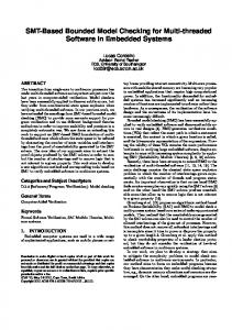
Recall that, according to our conventions, the local component φL and the global component φG are quantifier-free (ΣI ∪ ΣE )-formulae. In φG (i, d, d0 , j, e, e0 ) the variables i, d, d0 are called side parameters (these variables are instantiated in (3)-(4) by i, a[i], a0 [i], respectively) and the variables j, e, e0 are called proper parameters (these variables are instantiated in (3)-(4) by j, a[j], a0 [j], respectively). The intuition underlying the formula Update G (i, a, a0 ) defined by (4) is that the array a0 is obtained as a global update of the array a according to φG . In fact, in (4), the proper parameters of φG are instantiated as j, a[j], a0 [j], i.e. as the index to be updated, the old, and the new content of that index. Notice also that this updating is largely non-deterministic, because a T -formula like (3) does not univocally characterize the system evolution: this is revealed by the fact that φG is not a definable function, and by the fact that the side parameters d0 that may occur in φG are instantiated as the updated values a0 [i] (this circularity makes sense only if we view the T -formula (3) as expressing a constraint – not necessarily an assignment – for the updated array a0 ). In the remaining part of the paper, we fix an array-based system S = (a, I, τ ), in which the initial formula I is a ∀I -formula and the transition formula τ is a disjunction of T-formulae. Example 3.5. We present here the formalization into our framework of the Simplified Bakery Algorithm that can be found for instance in [3]. We take as TI the pure equality theory in the signature ΣI = {=}; to introduce TE , we analyze which kind of local data we need. The data e appearing in an array of processes are records consisting of the following two fields: (i) the field e.s represents the status (e.s ∈ {idle, wait, use, crash}); (ii) the field e.t represents the ticket (tickets range in the real interval [0, ∞), seen as a linear order with first element 0). Thus we need a two-sorted TE and two array variables in the language (or, a single array variable and a three-sorted TE , comprising a sort for the cartesian product): as pointed out above, such multi-sorted extensions of our framework are indeed straightforward. Models for TE are the obvious ones: one sort is interpreted as an enumerated datatype and the other sort is interpreted as the positive real domain. The initial formula I is ∀i (a[i].s = idle). The transition τ (a, a0 ) is the disjunction τ1 (a, a0 ) ∨ τ2 (a, a0 ) ∨ τ3 (a, a0 ), where the T -formulae τn (n ≤ 3) have the standard format from Definition 3.4 – namely ∃i (φnL (i, a[i], a0 [i]) ∧ Update nG (i, a, a0 )) – and the local and the global components φnL , φnG are specified in Figure 1 below. When formalizing the component transitions τ1 , τ2 , we use the approximation trick (see [2,3]): transitions τ1 , τ2 , in order to fire, would require a universally quantified guard which cannot be expressed in our format. We circumvent the problem by imposing that all the processes that are counterexamples to the guard go into a ‘crash’ state: this trick augments the possible runs of the system by introducing ‘spurious runs’, however if a safety property holds for the augmented ‘approximate’ system, then it also holds for the original system (the same is true for the recurrence properties of Section 6). a

Local components. The local components φn L , for n ≤ 3, are – φ1L :≡ a[i].s = idle ∧ a0 [i].s = wait ∧ a0 [i].t > 0 (the selected process goes from the state idle to wait and takes a nonzero ticket); – φ2L :≡ a[i].s = wait ∧ a0 [i] = huse, a[i].ti (the selected process goes from the state wait to use and keeps the same ticket); – φ3L :≡ a[i].s = use ∧ a0 [i] = hidle, 0i (the selected process goes from the state use to idle and the ticket is reset to zero). 0 0 Global components. The global components φn G (i, a[i], a [i], j, a[j], a [j]), for n ≤ 3, make case distinction as follows (the first case delegates the update to the local component):

– φ1G :≡ (j = i ∧ a0 [j] = a0 [i]) ∨ (j 6= i ∧ a[j].t < a[i].t ∧ a0 [j] = a[j]) ∨ (j 6= i ∧ a[j].t ≥ a[i].t ∧ a0 [j] = hcrash, a[j].ti) (if the selected process i goes from idle to wait, then any other process j keeps the same state/ticket, unless it has a ticket bigger or equal to the ticket of i – in which case j crashes); – φ2G :≡ (j = i ∧ a0 [j] = a0 [i]) ∨ (j 6= i ∧ (a[j].t > a[i].t ∨ a[j].t = 0) ∧ a0 [j] = a[j]) ∨ (j 6= i ∧ ¬(a[j].t > a[i].t ∨ a[j].t = 0) ∧ a0 [j] = hcrash, a[j].ti) (if the selected process i goes from wait to use, then any other process j keeps the same state/ticket, unless it has a nonzero ticket smaller than the ticket of i – in which case j crashes); – φ3G :≡ (j = i ∧ a0 [j] = a0 [i]) ∨ (j 6= i ∧ a0 [j] = a[j]) (if the selected process i goes from use to idle, then any other process keeps the same state/ticket).

Fig. 1. The Simplified Bakery Transition

4

Symbolic Representation and SMT solving

To make effective use of our framework, we need to be able to check whether certain requirements are met by a given array-based system. In other words, we A,I I ∀ need a powerful reasoning engine: it turns out that AE I -satisfiability of ∃ 5 sentences introduced below is just what we need. A,I I Theorem 4.1. The AE ∀ -sentences, i.e. of sentences of I -satisfiability of ∃ the kind

∃a1 · · · ∃an ∃i ∀j ψ(i, j, a1 [i], . . . , an [i], a1 [j], . . . , an [j]),

(5)

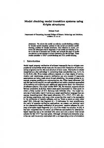
is decidable. We leave to [10] the detailed proof of the above theorem, here we focus on a discussion oriented to the employment of SMT-solvers in the decision procedure: Figure 2 depicts an SMT-based decision procedure for ∃A,I ∀I -sentences (in the simplified case in which only one variable of sort ARRAY occurs). 5

A,I I Decidability of AE ∀ -sentences plays in this paper a role similar I -satisfiability of ∃ to the Σ10 -decidability result employed in [4].

function AE I -check(∃a ∃i ∀j ψ(i, j, a[i], a[j])) t ←− compute-repsTI (i); φ ←− t = l; Atoms ←− IE(l) for each substitution σ mapping the j into the t’s do φ0 ←− purify(ψ(i, jσ, a[i], a[jσ])); φ ←− φ ∧ φ0 ; Atoms ←− Atoms ∪ atoms(φ0 ); end for each while Bool(φ) = sat do βI ∧ βE ∧ ηI ←− pick-assignment(Atoms, φ) (ρI , πI ) ←− TI -solver(βI ∧ ηIV ) (ρE , πE ) ←− TE -solver(βE ∧ l =l ∈ηI (es1 = es2 )) s1

s2

if ρI = sat and ρE = sat then return sat if ρI = unsat then φ ←− φ ∧ ¬πI if ρE = unsat then φ ←− φ ∧ ¬πE end while return unsat end

Fig. 2. The SMT-based decision procedure for ∃A,I ∀I -sentences

The set t of representative terms over i is computed by compute-repsTI (to simplify the matter, we can freely assume t ⊇ i). This function is guaranteed to exist since TI is effectively locally finite (for example, when ΣI contains no function symbol, compute-repsTI is the identity function). In order to purify formulae, we shall need below fresh index variables l abstracting the t and fresh element variables e abstracting the terms a[l]: the conjunction of the ‘defining equations’ t = l is stored as the formula φ, whereas the further defining equations a[l] = e (not to be sent to the Boolean solver) will be taken into account inside the second loop body. Then, the first loop is entered where we instantiate in all possible ways the universally quantified index variables j with the representative terms in the set t. For every such substitution σ, the formula ψ(i, jσ, a[i], a[jσ]) is purified by replacing the terms a[t] with the element variables e; after such purification, the resulting formula is added as a new conjunct to φ. Notice that this φ is a quantifier-free formula whose atoms are pure, i.e. they are either ΣI - or ΣE atoms. The function IE(l) returns the set of all possible equalities among the index variables l. Such equalities are added to the set of atoms occurring in φ as the TI - and TE -solvers need to take into account an equivalence relation over the index variables l so as to synchronize. We can now enter the second (and main) loop: the Boolean solver, by invoking the interface function pick-assignment inside the loop, generates an assignment over the set of atoms occurring in φ and IE(l). The loop is exited when φ is checked unsatisfiable (test of the while). The TI -solver checks for unsatisfiability the set βI of ΣI -literals in the Boolean assignment and the literals of the possible V partition ηI on l. Then, only the equalities {es1 = es2 | (ls1 = ls2 ) ∈ ηI } (and not also inequalities) among the purification variables e induced by the partition

ηI on l are passed to the TE -solver together with the set βE of ΣE -literals in the Boolean assignment (this is to take into account the congruence of a[l] = e). If both solvers detect satisfiability, then the loop is exited and AE I -check also returns satisfiability. Otherwise (i.e. if at least one of the solvers returns unsat), the negation of the computed conflict set (namely, πI or πE ) is conjoined to φ so as to refine the Boolean abstraction and the loop is resumed. If in the second loop, satisfiability is never detected for all considered Boolean assignments, then AE I -check returns unsatisfiability. The second loop can be seen as a refinement of the Delayed Theory Combination technique [5]. The critical point of the above procedure is the fact that the first loop may produce a very large φ: in fact, even in the most favourable case in which compute-repsTI is the identity function, the purified problem passed to the solvers of the second loop has exponential size (this is consequently the dominating cost of the whole procedure, see [10] for complexity details). To improve performances, an incremental approach is desirable: in the incremental approach, the second loop may be entered before all the possible substitutions have been examined. If the second loop returns unsat, one can exit the whole algorithm and only in case it returns sat further substitutions (producing new conjuncts for φ) are taken into consideration. Since when AE I -check is called in conclusive steps of our model checking algorithms (for fixpoint, safety, or progress checks), the expected answer is unsat, this incremental strategy may be considerably convenient. Other promising suggestions for reducing the number of instantiations (in the case of particular index and elements theories) come from recent decision procedures for fragments of theories of arrays, see [6,11].

5

Safety Model Checking

Checking safety properties means checking that a set of ‘bad states’ (e.g., of states violating the mutual exclusion property) cannot be reached by a system. This can be formalized in our settings as follows: Definition 5.1. Let K(a) be an ∃I -formula (whose role is that of symbolically representing the set of bad states). The safety model checking problem for K is the problem of deciding whether there is an n ≥ 0 such that the formula I(a0 ) ∧ τ (a0 , a1 ) ∧ · · · ∧ τ (an−1 , an ) ∧ K(an )

(6)

is AE I -satisfiable. If such an n does not exist, K is safe; otherwise, it is unsafe. Notice that the AE I -satisfiability of (6) means precisely the existence of a finite run leading from a state in I to a state in K. 5.1

Backward Reachability

If a bound for n in the safety model checking is known a priori, then safety can be decided by checking the AE I -satisfiability of suitable instances of (6) (this is

possible because each formula (6) is equivalent to a ∃A,I ∀I -formula). Unfortunately, this is rarely the case and we must design a more refined method. In the following, we adapt algorithms that incrementally maintain a representation of the set of reachable states in an array-based system. Definition 5.2. Let K(a) be an ∃I -formula. An M-state s0 is backward reachable from K in n steps iff there exists a sequence of M-states s1 , . . . , sn such that M |= τ (s0 , s1 ) ∧ · · · ∧ τ (sn−1 , sn ) ∧ K(sn ). We say that s0 is backward reachable from K iff it is backward reachable from K in n steps for some n ≥ 0. Before designing our backward reachability algorithm, we must give a symbolic representation of the set of backward reachable states. Preliminarily, notice that if K(a) is an ∃I -formula, the set of states which are backward reachable in one step from K can be represented as follows: P re(τ, K) := ∃a0 (τ (a, a0 ) ∧ K(a0 )).

(7)

Although P re(τ, K) is not an ∃I -formula anymore, we are capable of finding an equivalent one in the class: Proposition 5.3. Let K(a) be an ∃I -formula; then P re(τ, K) is AE I -equivalent to an (effectively computable) ∃I -formula K 0 (a). The proof of this Proposition can be obtained by a tedious syntactic computation while using (2) together with the fact that TE admits quantifier elimination. Abstractly, the set of states that can be backward reachable from K can be recursively characterized as follows: (a) P re0 (τ, K) := P ren+1 (τ, K) := WnK and (b) n n s P re(τ, P re (τ, K)). The formula BR (τ, K) := s=0 P re (τ, K) (having just one free variable of type ARRAY) symbolically represents the states that can be backward reached from K in n steps. The sequence of BRn (τ, K) allows us to rephrase the safety model checking problem (Definition 5.1) using symbolic representations by saying that K is safe iff the formulae I ∧ BRn (τ, K) are all not AE I -satisfiable. This still requires infinitely many tests, unless there is an 6 n such that the formula ¬(BRn+1 (τ, K) → BRn (τ, K)) is AE I -unsatisfiable. n n+1 The key observation now is that both I ∧ BR (τ, K) and ¬(BR (τ, K) → BRn+1 (τ, K)) can be easily transformed into ∃A,I ∀I -formulae so that their AE I satisfiability is decidable and checked by the procedure AE -check of Figure 2. I This discussion suggests the adaptation of a standard backward reachability algorithm (see, e.g., [12]) depicted in Figure 3, where Pre takes a formula, it computes Pre as defined in (7), and then applies the required syntactic manipulations to transform the resulting formula into an equivalent one according to Proposition 5.3. 6

n n+1 Notice that the AE (τ, K)) is obvious by I -unsatisfiability of ¬(BR (τ, K) → BR n+1 definition. Hence, the AE -unsatisfiability of ¬(BR (τ, K) → BRn (τ, K)) implies I n+1 that AE (τ, K) ↔ BRn (τ, K). I |= BR

function BReach(K) i ←− 0; BR0 (τ, K) ←− K; K 0 ←− K 0 if AE I -check(BR (τ, K) ∧ I) = sat then return unsafe repeat K i+1 ←− Pre(τ, K i ) BRi+1 (τ, K) ←− BRi (τ, K) ∨ K i+1 i+1 if AE (τ, K) ∧ I) = sat then return unsafe I -check(BR else i ←− i + 1 i+1 until AE (τ, K) → BRi (τ, K)) = unsat I -check(¬(BR return safe end

Fig. 3. Backward Reachability for Array-based Systems Theorem 5.4. Let K(a) be an ∃I -formula; then the function BReach in Figure 3 semi-decides the safety model checking problem for K. Example 5.5. In the Simplified Bakery example of Figure 1 (with the formula K to be tested for safety given like in (1)), the algorithm of Figure 3 stops after four loops and certifies safety of K. a 5.2

Termination of Backward Reachability

Indeed, the main problem with the semi-algorithm of Figure 3 is termination; in fact, it may not terminate when the system is safe. In the literature, termination of infinite state model checking is often obtained by defining a well-quasi-ordering (wqo – see, e.g., [1]) on the configurations of the system. Here, we adapt this approach to our setting, by defining model-theoretically a notion of configuration and then introducing a suitable ordering on configurations: once this is done, it will be immediate to prove that termination follows whenever the ordering among configurations is a wqo. An AE I -configuration (or, briefly, a configuration) is an M-state in a finite index model M of AE I : a configuration is denoted as (s, M), or simply as s, leaving M implicit. Moreover, we associate a ΣI -structure sI and a ΣE -structure sE with an AE I -configuration (s, M) as follows: the ΣI -structure sI is simply the finite structure MI , whereas sE is the ΣE -substructure of ME generated by the image of s (in other words, if INDEXM = {c1 , . . . , ck }, then sE is generated by {s(c1 ), . . . , s(ck )}). We remind few definitions about preorders. A preorder (P, ≤) is a set endowed with a reflexive and transitive relation; an upset of such a preorder is a subset U ⊆ P such that (p ∈ U and p ≤ q imply q ∈ U ). An upset U is finitely generated iff it is a finite union of cones, where a cone is an upset of the form ↑ p = {q ∈ P | p ≤ q} for some p ∈ P . A preorder (P, ≤) is a well-quasi-ordering (wqo) iff every upset of P is finitely generated (this is equivalent to the standard definition, see [10]). We define now a preorder among our configurations:

Definition 5.6. Let s, s0 be configurations; s0 ≤ s holds iff there are a ΣI embedding µ : s0I −→ sI and a ΣE -embedding ν : s0E −→ sE such that the set-theoretical compositions of µ with s and of s0 with ν are equal. Let K(a) be an ∃I -formula: we denote by [[K]] the set of AE I -configurations satisfying K; in symbols, [[K]] := {(M, s) | M |= K(s)}. Proposition 5.7. For every ∃I -formula K(a), the set [[K]] is upward closed; also, for every ∃I -formulae K1 , K2 , we have [[K1 ]] ⊆ [[K2 ]] iff AE I |= K1 → K2 . The set of configurations B(τ, K) which are backward reachable from a given ∃I formula K is thus an upset, being the union of infinitely many upsets; however, even in case the latter are finitely generated, B(τ, K) needs not be so. Under the hypothesis of local finiteness of TE , this is precisely what characterizes termination of backward reachability search: Theorem 5.8. Assume that TE is locally finite; let K be an ∃I -formula. If K is safe, then BReach in Figure 3 terminates iff B(τ, K) is a finitely generated upset.7 As a consequence, BReach always terminates when the preorder on AE I configurations is a wqo. The termination result of Theorem 5.8 covers many well-known special cases, like broadcast protocols, some versions of the bakery algorithm, lossy channel systems (notice that for the latter, there doesn’t exist a primitive recursive complexity lower bound); to apply Theorem 5.8, one needs classical facts like Dikson’s Lemma, Higman’s Lemma, Kruskal’s Theorem, etc. (see again [10] for details).

6

Progress Formulae for Recurrence Properties

Liveness problems are difficult and even more so for infinite state systems. In the following, we consider a special kind of liveness properties, which falls into the class of recurrence properties in the classification introduced in [13]. Our method for dealing with such properties consists in synthesizing progress functions definable at quantifier free level. A recurrence property is a property which is infinitely often true in every infinite run of a system; in other words, to check that R is a recurrence property it is sufficient to show that it cannot happen that there is an infinite run s0 , s1 , . . . , si , . . . such that R is true at most in the states from a finite prefix s0 , . . . , sm . This can be formalized in our framework as follows. Definition 6.1. Suppose that R(a) is a ∀I -formula; let us use the abbreviations K(a) for ¬R(a) and τK (a, a0 ) for τ (a, a0 ) ∧ K(a) ∧ K(a0 ).8 We say that R is a recurrence property iff for every m the infinite set of formulae I(b1 ), τ (b1 , b2 ), . . . , τ (bm , a0 ), τK (a0 , a1 ), τK (a1 , a2 ), . . . 7

8

(8)

If K is unsafe, we already know that BReach terminates because it detects unsafety (cf. Theorem 5.4). Notice that τK is easily seen to be equivalent to a disjunction of T -formulae, like the original τ .

is not satisfiable in a finite index model of AE I . The finite prefix I(b1 ), τ (b1 , b2 ), . . . , τ (bm , a0 ) in (8) above ensures that the states assigned to a0 , a1 , . . . are (forward) reachable from an initial state, whereas the infinite suffix τK (a0 , a1 ), τK (a1 , a2 ), . . . expresses the fact that property R is never attained. Observe that, whereas it can be shown that the AE I -satisfiability of (6) for safety problems (cf. Definition 5.1) is equivalent to its satisfiability in a finite index model of AE I , this is not the case for (8). This imposes the above explicit restriction to finite index models since, otherwise, recurrence might unnaturally fail in many concrete situations. Example 6.2. In the Simplified Bakery example of Figure 1, we take K to be ∃i (i = d ∧ a[i] = wait) (here d is a fresh constant of type ΣI ). Then the AE I -satisfiability of (8) implies that the protocol cannot guarantee absence of starvation. a Let R be a recurrence property; we say that R has polynomial complexity iff there exists a polynomial f (n) such that for every m and for k > f (n) the formulae I(b1 ) ∧ τ (b1 , b2 ) ∧ · · · ∧ τ (bm , a0 ) ∧ τK (a0 , a1 ) ∧ · · · ∧ τK (ak−1 , ak )

(9)

are all unsatisfiable in the models M of AE I such that the cardinality of the support of MI is at most n (in other words, f (n) gives an upper bound for the waiting time needed to reach R by a system consisting of less than n processes). Definition 6.3. Let R(a) be a ∀I -formula and let K and τK be as in Definition 6.1. A formula ψ(t(j), a[t(j)]) is an index invariant iff there exists a safe ∃I formula H such that AE I |= ∀a0 ∀a1 ∀j (¬H(a0 ) ∧ τK (a0 , a1 ) → (ψ(t, a0 [t]) → ψ(t, a1 [t]))).

(10)

A progress condition for R is a finite set of index invariant formulae ψ1 (t(j), a[t(j)]), . . . , ψc (t(j), a[t(j)]) for which there exists a safe ∃I -formula H such that AE I |= ∀a0 ∀a1 ¬H(a0 )∧τK (a0 , a1 ) → ∃j

c _


(¬ψk (t, a0 [t]) ∧ ψk (t, a1 [t])) . (11)

k=1

Suppose there is a progress condition as above for R; if M is a model of AE I such that the support of MI has cardinality at most n, then the formula (9) cannot be satisfiable in M for k > c · n` (here ` is the length of the tuple j). This argument shows the following: Proposition 6.4. If there is a progress condition for R, then R is a recurrence property with polynomial complexity.

Example 6.5. In the Simplified Bakery example of Example 6.2, the following four index invariant formulae: a[j].s = crash a[j].t > a[d].t

a[j].t = 0 ∨ a[j].t > a[d].t ¬(a[j].t < a[d].t ∧ a[j].s = wait)

constitute a progress condition, thus guaranteeing that each non faulty process d can get (in polynomial time) the resource every time it asks for it. The algorithm of Figure 3 is needed for certifying safety of some formulae (like ∃i (a[i].s = use ∧ a[i].t = 0)) to be used as the H of Definition 6.3. a Let us now discuss how to mechanize the application of Proposition 6.4. The validity tests (10) and (11) can be reduced to unsatisfiability tests covered by Theorem 4.1; however, the search space for progress conditions looks to be unbounded for various reasons (the number of the ψ’s of Definition 6.3, the length of the string j, the ‘oracle’ safe H’s, etc.). Nevertheless, the proof of the following unexpected result shows (in the appropriate hypotheses) how to find progress conditions whenever they exist: Theorem 6.6. Suppose that TE is locally finite and that safety of ∃I -formulae can be effectively checked. Then the existence of a progress condition for a given ∀I -formula R is decidable.

7

Related work and Conclusions

A popular approach to uniform verification (e.g., [2,3,4]) consists of defining a finitary representation of the (infinite) set of states and then to explore the state space by using such a suitable data structure. Although such a data structure may contain declarative information (e.g., constraints over some algebraic structure or first-order formulae), a substantial part is non-declarative. Typically, the part of the state handled non-declaratively is that of indexes (which, for parametrized systems, specify the topology), thereby forcing to re-design the verification procedures whenever their specification is changed (for the case of parametrized systems, whenever the topology of the systems changes). Since our framework is fully declarative, we avoid this problem altogether. There has been some attempts to use a purely logical techniques to check both safety and liveness properties of infinite state systems (e.g., [7,9]). The hard part of these approaches is to guess auxiliary assertions (either invariants, for safety, or ranking functions, for liveness). Indeed, finding such auxiliary assertions is not easy and automation requires techniques adapted to specific domains (e.g., integers). In this paper, we have shown how our approach does not require auxiliary invariants for safety and proved that the search for certain progress conditions can be fully mechanized (Theorem 6.6). In order to test the viability of our approach, we have built a prototype implementation of the backward reachability algorithm of Figure 3. The function AE I -check has been implemented by using a naive instantiation algorithm and

a state-of-the-art SMT solver. We have also implemented the generation of the proof obligations (10) and (11) for recognizing progress conditions. This allowed us to automatically verify the examples discussed in this paper and in [10]. We are currently planning to build a robust implementation of our techniques.

References 1. P. A. Abdulla, K. Cerans, B. Jonsson, and Y.-K. Tsay. General decidability theorems for infinite state systems. In Proc. of LICS ’96, pages 313–321, 1996. 2. P. A. Abdulla, G. Delzanno, N. Ben Henda, and A. Rezine. Regular model checking without transducers. In Proc of TACAS ’07, volume 4424 of LNCS, pages 721–736. Springer, 2007. 3. P. A. Abdulla, G. Delzanno, and A. Rezine. Parameterized verification of infinitestate processes with global conditions. In Proc. of CAV ’07, volume 4590 of LNCS, pages 145–157. Springer, 2007. 4. A. Bouajjani, P. Habermehl, Y. Jurski, and M. Sighireanu. Rewriting systems with data. In Proc. of FCT ’07, volume 4639 of LNCS, pages 1–22. Springer, 2007. 5. M. Bozzano, R. Bruttomesso, A. Cimatti, T. A. Junttila, S. Ranise, P. van Rossum, and R. Sebastiani. Efficient theory combination via boolean search. Information and Computation, 204(10):1493–1525, 2006. 6. A. R. Bradley, Z. Manna, and H. B. Sipma. What’s decidable about arrays? In Proc. of VMCAI ’06, volume 3855 of LNCS, pages 427–442. Springer, 2006. 7. L. M. de Moura, H. Rueß, and M. Sorea. Lazy theorem proving for bounded model checking over infinite domains. In Proc. of CADE ’02, volume 2392 of LNCS, pages 438–455. Springer, 2002. 8. H. B. Enderton. A Mathematical Introduction to Logic. Academic Press, New York-London, 1972. 9. Y. Fang, N. Piterman, A. Pnueli, and L. D. Zuck. Liveness with invisible ranking. Software Tools for Technology, 8(3):261–279, 2006. 10. S. Ghilardi, E. Nicolini, S. Ranise, and D. Zucchelli. Towards SMT model checking of array-based systems. Technical Report RI318-08, Universit` a degli Studi di Milano, 2008. Available at http://homes.dsi.unimi.it/~zucchell/publications/ techreport/GhiNiRaZu-RI318-08.pdf. 11. C. Ihlemann, S. Jacobs, and V. Sofronie-Stokkermans. On local reasoning in verification. In Proc. of TACAS ’08, volume 4963 of LNCS, pages 265–281. Springer, 2008. 12. Y. Kesten, O. Maler, M. Marcus, A. Pnueli, and E. Shahar. Symbolic model checking with rich assertional languages. Theoretical Computer Science, 256(12):93–112, 2001. 13. Z. Manna and A. Pnueli. A hierarchy of temporal properties. In Proc. of PODC ’90, pages 377–410. ACM Press, 1990. 14. R. Nieuwenhuis, A. Oliveras, and C. Tinelli. Solving SAT and SAT Modulo Theories: From an abstract Davis–Putnam–Logemann–Loveland procedure to DPLL(T ). Journal of the ACM, 53(6):937–977, 2006. 15. T. Rybina and A. Voronkov. A logical reconstruction of reachability. In Proc. of PSI ’03, volume 2890 of LNCS, pages 222–237. Springer, 2003. 16. R. Sebastiani. Lazy satisfiability modulo theories. Journal on Satisfiability, Boolean Modeling and Computation, 3:141–224, 2007.