Tracking Data Structures Coherency in Animated Ray Tracing for Real-Time 3D-Rendering Sajid Hussain
Håkan Grahn
Department of Systems and Software Engineering Blekinge Institute of Technology, Sweden
[email protected]
Department of Systems and Software Engineering Blekinge Institute of Technology, Sweden
[email protected]
Abstract— Ray tracing is a well known method for photorealistic image synthesis, volume visualization and rendering. Over the last decade the method is being adopted throughout the research community around the world. With the advent of the high speed processing units, the method has been emerging from offline rendering towards real time rendering. The success behind ray tracing algorithms lies in the use of acceleration data structures and modern processing power of CPUs and GPUs. kd-tree is one of the most widely used data structures based on surface area heuristics (SAH). The major bottleneck in kd-tree construction is the time consumed to find optimum split locations. In this paper, we propose a prediction algorithm for animated ray tracing based on Kalman filtering. The algorithm successfully predicts the split locations for the next consecutive frame in the animation sequence. Thus, giving good initial starting points for one dimensional search algorithms to find optimum split locations – in our case parabolic interpolation combined with golden section search. With our technique implemented, we have reduced the “running kd-tree construction” time by between 78% and 87% for dynamic scenes with 16.8K and 252K polygons respectively. Keywords-component; Ray Tracing; Tracking; Kalman Filter
I.
INTRODUCTION
Ray tracing is one of the most widely used algorithms for interactive graphics applications and geometric processing. The performance of these algorithms is accelerated by using bounding volume hierarchies (BVH). BVHs are efficient data structures used for intersection tests or culling in computer graphics. Ray tracing algorithms compute and transverse BVHs in real time to perform intersection test. While ray tracing has evolved into a real time image synthesis technique in the last decade, more efficient hardware, effective acceleration structures and more advanced transversal algorithms have contributed to the increased performance. Among different acceleration structures [3][4], kd-trees have given better or at least comparable performance in terms of speed as compared to others [1]. These structures are more efficient if built using surface area heuristics (SAH) [2]. Interactive ray tracing demands fast construction of BVHs but an optimized fast construction of kd-tree is very expensive for large dynamic scenes. Although, efforts are being made to optimize kd-tree construction for large dynamic scenes [5][6][7][8][9], there still lies a gulf between kd-tree construction and interactive large dynamic scene applications.
In this paper, we present an approach to improve and optimize the construction of kd-trees for ray tracing of dynamic scenes. We are concerned about the decision of the separation plane location. In most of the dynamic scenes used in research, consecutive frames do not depict considerable differences in terms of geometry information. Our approach is to make use of this particular property for constructing kd-tree structures. We start with the approach used in [9] for static scenes, where parabolic interpolation is combined with golden section search to reduce the amount of work done when building the kd-trees. We further extend this approach for dynamic scenes and make use of the vector Kalman filter to predict the split locations for the next consecutive frame. The same golden section search and parabolic interpolation is then used to find the minimum but this time the predicted location is used as a starting point, hence reducing the number of steps used to find the minimum of the parabolic cost function. We have evaluated our technique against a standard SAH algorithm for dynamic scenes with varying complexities and behaviors. With our algorithm, we have achieved average kd-tree built times of 30msec for 1617k triangles scene and 210msec for 252k triangles scene. This corresponds to a reduction of the kd-tree construction time by between 78% and 87%. The rest of the paper is organized as follows. Section 2 gives some related research work on kd-tree construction followed by the theory behind SAH based kd-trees in section 3. We describe the mathematics behind the Kalman filter in section 4 along with our proposed technique in section 5. Section 6 gives our implementation results and some discussion. We conclude the paper in section 7 with future work. II.
RELATED WORK
kd-tree construction has mainly focused on optimized data structure generation for fast ray tracing. The state-of-theart O ( n log n ) algorithm has been analyzed in depth by [10] and [11]. Further in [12], the theoretical and practical aspects of ray tracing including kd-tree cost function modeling and experimental verifications have been described. Current work in [5] and [13] also aims at fast construction of kd-trees. By adaptive sub-sampling they approximate the SAH cost function by a piecewise quadratic function.
There are many different other implementations of the kdtree algorithm using SIMD instructions like in [14]. Another approach is used by [15], where the author experiments with stream kd-tree construction and explores the benefits of parallelized streaming. Both [5] and [15] demonstrate considerable improvements as compared to conventional SAH based kd-tree construction. The cost function to optimally determine the depth of the subdivision in kd-tree construction has been demonstrated by several authors. In [16], the authors derive an expression that confirms that the time complexity is less dependent on the number of objects and more on the size of the objects. They calculate the probability that the ray intersects an object as a function of the total area of the subdivision cells that (partly) contain the object. In [2], the authors use a similar strategy but refine the method to avoid double intersection tests of the same ray with the same object. They determine the probability that a ray intersects at least one leaf cell from the set of leaves within which a particular object resides. They use a cost function to find the optimal cutting planes for a kd-tree construction. A similar method was also implemented in [17]. Recently, kd-tree acceleration structures for modern graphics hardware have been proposed in [8] and [18], where they experimented with kd-tree acceleration structure for GPU ray tracers and achieved considerable improvement. III.
SAH BASED KD-TREE CONSTRUCTION
In this section, we give some background about the kd-tree algorithm, which will be the foundation for the rest of the paper. Consider a set of points in a space Rd, the kd-tree is normally built over these points. In general, kd-trees are used as a starting point for optimized initialization of k-means clustering [19] and nearest neighbour query problems [20]. In computer graphics, and especially in ray tracing applications, kd-trees are applied over a scene S with points as bounding boxes of scene objects. The kd-tree algorithm subdivides the scene space recursively. For any given node Lnode of the kd-tree, a splitting plane splits the bounding box of the node into two halves, resulting in two bounding boxes, left and right. These are called child nodes and the process is repeated until a certain criterion is met. In [1], the author reports that the adaptability of the kd-tree towards the scene complexity can be influenced by choosing the best position of the splitting plane. The choice of the splitting plane is normally the mid way between the scene maximum and minimum along a particular coordinate axis [21] and a particular cost function is minimized. In [2], SAH is introduced for the kd-tree construction algorithm which works on probabilities and minimizes a certain cost function. The cost function is built by firing an arbitrary ray through the kd-tree and applying some assumptions. Figure 1 uses the conditional probability P(y|x) that an arbitrary fired ray hits the region y inside region x provided that it has already touched the region x. Bayes rule can be used to calculate the conditional probability P(y|x) as
P( y | x ) =
P( x | y ) P( y ) . P( x )
(1) Ray
y x Figure 1. Visualization of Conditional Probability P(y|x).
P(x|y) is the conditional probability that the ray hits the region x provided that it has intersected y, and here P(x|y) = 1. P(x) and P(y) can be expressed in terms of areas [1]. If we start from the root node or the parent node and assume that it contains N elements and the ray passing the root node has to be tested for intersection with N elements. If we assume that the computational time it takes to test the ray intersection with element n ⊆ N is Tn, then the overall computational cost C of the root node would be N
C = ∑ Tn .
(2)
n =1
After further division of root node, the ray intersection test cost for each left and right child nodes changes to CLeft and CRight. Thus the overall new cost becomes CTotal and (3) CTotal = CTrans + CRight + CLeft . Where CTrans is the cost of traversing the parent or root node and N Left
N Right
i =1
j =1
CTotal = CTrans + PLeft . ∑ Ti + PRight . ∑ T j ,
(4)
where A and PRight = Right . (5) A A Where A is the surface area of the root node and the area of two child nodes are ALeft and ARight. PLeft and PRight are the probabilities of a ray hitting the left and the right child nodes. NLeft and NRight are the number of objects present in the two nodes and Ti and Tj are the computational time for testing ray intersection with the ith and jth objects of the two child nodes. The kd-tree algorithm minimizes the cost function CTotal, and then subdivides the child nodes recursively. As shown in [15], the cost function is a bounded variation function as it is the difference of two monotonically varying functions CLeft and CRight. In [15], this important property of the cost function has been exploited to increase the approximation accuracy of the cost function and only those regions that can contain the minimum have been adaptively sampled. We have used the technique in [9], called golden section search, to find out the region that could contain the minimum and combined it with parabolic interpolation to search for the minimum. Further, we predict the minimums of the cost function (split locations) for next consecutive frame using the Kalman filter. We use predicted split locations as starting points for kd-tree construction over consecutive frames. In the next section, we present some mathematics behind the Kalman filter. PLeft =
ALeft
IV.
THE KALMAN FILTER
The Kalman filter is named after its inventor Kalman in 1960 [22]. The Kalman filter presents a recursive approach to discrete data linear filtering and prediction problems. The filter estimates the state of an underlying discrete time controlled process x ∈ ℜ n which is presented by the following difference equation xk = Axk −1 + Buk −1 + wk −1 , (6) with the measurement or observation z ∈ℜ m and presented by zk = Hxk + vk .
(7)
The random variables wk and vk are process and measurement noises respectively and assumed to be independent, white and normally distributed with zero mean and covariance matrices Q and R . p ( w ) ≈ N ( 0, Q ) p ( v ) ≈ N ( 0, R )
.
(8)
Matrix A in equation 6 is an n × n matrix and it represents the state relationship from previous time step k − 1 to current time step k . The n × 1 matrix B relates the optional control input u to the state x . The m × n matrix H in equation 8 relates the state xk to the measurement zk . A more detailed introduction about the Kalman filter could be found in any good book on the Kalman filter, we will just describe some basic steps of the filter. The Kalman filter has two main steps called time update (prediction) and measurement update (correction). The prediction state projects the current state estimate ahead in time and the correction state adjusts the projected estimate by an actual measurement at that time. The filter prediction and update steps are described as follows (the details could be found in [23] along with the derivation). Prediction ∧−
∧
x k = A x k −1 + Buk −1
.
(9)
. ∧ ∧− ∧− ⎞ ⎛ x k = x + K k ⎜ zk − H x ⎟ ⎝ ⎠ Error Covariance Correction
(10)
Error Covariance Projection Pk − = APk −1 AT + Q Kalman Gain K k = Pk H T ( HPk H T + R )
−1
State Ahead Correction
Pk = ( I − K k H ) Pk−
V.
FAST CONSTRUCTION OF KD-TREES
We combine golden section search and parabolic interpolation [9] with the Kalman filter to construct kd-trees for animated ray tracing. We take advantage of the fact that adjacent frames in animated ray tracing do not depict a dramatic change in most of the animated scenes (we are
talking about scenes normally used by the research community in computer graphics). The algorithm we present here is simple to describe. In our algorithm, we start with the technique described in [9] and construct the kd-tree for the first frame of an animated scene. We then use a Kalman filter to predict split locations for the next consecutive frame. The algorithm also keeps track of kd-tree depth and split orientations. We then apply golden section combined with parabolic interpolation for a one dimensional search of split plane but this time the starting point for the one dimensional search is the predicted split location. This gives us a very fast convergence towards the cost function optimum. The beauty of the Kalman filter is that we do not need any previous history to predict the future. This gives us memory free prediction. What we do need is the memory to store the predicted values in the prediction step of the Kalman filter. The same memory locations are updated during the update step. Algorithm 1 shows the pseudo code for the Kalman filter, where we initialize the parameters to their default initial values and predict the future states. Note that in the Kalman filter step, we use initial split positions information from the first frame and add measurement noise to construct virtual next observations. We then predict the actual split positions for the next frame based on these virtual next observations. In the last step, we update the information for the Kalman filter parameters based on actual split locations information returned by the one dimensional search Algorithm 2. The OptSplit function in Algorithm 2 takes KalmanStruct which includes all the information about Kalman Orientation (KalmanOrient), Kalman Depth (KalmanDepth) and Kalman predicted optimum split location (KalmanStartPt). The KalmanOrient and the KalmanDepth are the two variables used to track the axis orientation for particular depth for Kalman filter. The algorithm itself finds the optimal split orientation for a given depth information and compares it with that of the Kalman Orientation. If the two orientations match, the algorithm uses the start point as predicted by the Kalman filter. Otherwise, it starts looking for an optimum from extreme positions. The Kalman Orientation (KalmanOrient) and the Kalman Depth (KalmanDepth) are the two vectors which store the orientation and corresponding depth information from the previous consecutive frame. The objective behind the orientation match is to track the requirements for orientation change because of the dynamic scene. If there is no match, we update the Klaman filter parameters with the new orientation and apply the one dimensional search algorithm starting from extreme boundaries of the particular bounding box. Algorithm 1 – The Kalman Filter // Kalman filter initialization parameters // State vector x and covariance P apriori estimate S.x = 0 and S.P = 0; // Input control vector u and Input matrix B S.u = 0 and S.B = 0; S.A = 1; // State transition matrix // Covariance of process noise Q S.Q = Std[InitSplitPos InitSplitPos*p(w)]^2;
S.H = 1; // Observation matrix H // Measurement noise covariance S.R = Std_Dev[InitSplitPos - InitSplitPos*p(v)]^2; // Kalman Filter function KalmanFilter(S(k)) True(k) = InitSplitPos(k) // Construct measurement S.z(k) = True(k)+p(v)*True(k); Time update as in equation 10 Measurement update as in equation 11 return S(k+1) end function
Algorithm 2 – Optimum Split Search function OptSplit(Polygons,AABB,KalmanStruct) Orient = OptSplitOrient(Polygons); // Predict the next split location KalmanStartPt = KalmanFilter(S(k)); if (Orient = KalmanOrient and Depth = KalmanDepth) Optimum = OptSearch(Polygons, AABB, KalmanOrient, KalmanStartPt); else Optimum = OptSearch(Polygons, AABB, Orient); return Optimum; end function
VI.
RESULTS AND DISCUSSION
We have tested our algorithm on a variety of animation sequences as shown in Figure 2. The scenes differ with triangular count and animation behaviour. The scenes consist of regularly sized and uniformly distributed triangles. We ran our kd-tree construction algorithm and recorded the Kalman prediction accuracy and the time our algorithm took to build kd-tree for each frame in the sequence. We have chosen MATLAB® and C++ for implementation of our algorithm. We have implemented the Kalman filter prediction routine in MATLAB® and the kd-tree construction routine in C++. The kd-tree construction is linked in MATLAB® through Dynamic Link Library (DLL). Routines for PLY file reading are also implemented in MATLAB®. The timing results shown in this paper are only for kd-tree construction in DLL. We have performed all the simulations on a workstation with an Intel Core2 CPU, 2.16 GHz processor and 2GB of RAM. The scenes we have used in our simulations vary in terms of their complexities and behaviours. Figure 2 shows four different animation sequences. In Figure 3 and Figure 4, we analyze how the cost functions change in the horse (16.8K 48 Frames) and bunny-dragon (252.5K - 16 Frames) animations for the two axis (y and z) as shown in Figure 2 and for only root node split positions. We also plot the actual and predicted split positions of the Kalman filter. Note that the actual split positions have been calculated on basis of Surface Area Heuristics (SAH). Let’s analyse Figure 3 closely, the upper two sub-figures in Figure 3 (left to right) show the cost function shift for each frame in the horse animation sequence for y and z axis respectively. The minimums of these parabolic cost functions are the optimum split plan locations. The bottom two subfigures in Figure 3 (left to right) show how the actual optimum split plan locations change over time, the predicted split plan
locations by the Kalman filter (time is no. of frames in this case) for y and z axis respectively. The red dots are the virtual measurement observations constructed through measurement noise p ( v ) added (equation 8) and the term responsible for constructing these observations in Algorithm 1 is S . z ( k ) = True ( k ) + p ( v ) × True ( k ) . Also note the periodic behaviour of split plan locations change as the horse animation sequence is periodic in nature. Our algorithm has successfully predicted the split plan locations for consecutive frames. Hence, it provides a good initial guess for one dimensional search (parabolic interpolation combined with golden section search). If we closely analyse the prediction curves, we see that in almost all the cases, the prediction error is very small. Since, the entire scene dataset exhibits a strong coherency between consecutive frames; we have successfully exploited this property here. Although, in all these scenes, there remain a constant number of polygons (triangles) throughout a particular animation sequence, we see a random behaviour in the kd-tree build time. The phenomenon occurs due to random noise added by the Kalman filter prediction steps as in Algorithm 1, where we have constructed the virtual observations by adding the measurement noise from equation 8. The added noise maximum error difference is not greater than 1msec. Table 1 shows the time difference between an initial build and a running build of kd-tree data structures for each animation sequence used in this paper. See the considerable improvement in the build time in running mode. We have not yet added the overhead of the Kalman filter in Table 1. In MATLAB®, the Kalman filter’s average aggregated overhead is approx. 400-450msec for the whole sequence of 50 frames with average of 84K polygons (triangles) in each frame. We expect this time down to 100-150msec if efficiently implemented in C++. So, in worst case we could add 3-5msec per frame. TABLE I.
CONVENTIONAL VS MODIFIED KD-TREE BUILD TIME
Scene
Polygons
Normal kd-Tree Build (msec)
Horse Elephant ClothBall Bunny Dragon
16.8K 84.6K 92.2K 252.5K
135 710 802 1610
Modified kd-Tree Build (msec) Initial Running Build Build 135 30 710 105 802 120 1610 210
Time Reduc ed 78% 85% 85% 87%
VII. CONCLUSION AND FUTURE WORK We have presented an algorithmic speedup technique for fast kd-tree construction for animated ray tracing. The optimum split location search for kd-tree construction is the main time consuming job. As many of the animation sequences used by the research community for animated ray tracing exhibit strong data structures coherency properties, we have made use of a Kalman filter for predicting the next possible data structure (kd-tree in our case) state of the animated sequence. We use here the vector Kalman filter and load it with initial split plan
locations (we build kd-tree for starting frame in the sequence based on the technique described in [9]). The vector Kalman filter then predicts the next possible split locations for the next frame in the sequence. The prediction error is very small as we can see in the above sample simulation pictures. We use these predicted locations as starting points for the one dimensional optimum search algorithm. With best initial guess, the algorithm exhibits very fast convergence and we see the results quite promising for the running kd-tree build time as compared to static or initial kd-tree build. We achieve 78% to 87% increase in kd-tree construction time for the scenes with as low as 17K and as high as 252K polygons. We have implemented our proposed model in MATLAB® and C++. Main prediction engine of the Kalman filter is implemented in MATLAB®. C++ handles the kd-tree construction routines. We have used five different animation sequences with a varying number of complexities and behaviours i.e., between 17K to 252K primitives and 16 to 73 frames. We have demonstrated a considerable decrease in build time as compared to standard SAH based kd-tree. Further use of the technique could be demonstrated on scenes with varying number of complexities in connective frames and scenes with non-uniform polygons distribution. REFERENCES
[8] T Foley and J Sugerman. kd-tree Acceleration Structures For A GPU [9] [10] [11] [12] [13] [14] [15] [16] [17]
[18]
[1] V. Havran. Heuristic Ray Shooting Algorithms. PhD thesis, Faculty of Electrical Engineering, Czech Technical University in Prague, 2001.
[2] J. D. MacDonald and K. S. Booth. Heuristics for Ray Tracing Using [3] [4] [5] [6] [7]
Space Subdivision. In Graphics Interface Proceedings 1989, pages 152– 163, Wellesley, MA, USA, June 1989. A.K. Peters, Ltd. G. Stoll.: Part I: Introduction to Realtime Ray Tracing. SIGGRAPH 2005 Course on Interactive Ray Tracing, 2005. J. Zara.: Speeding Up Ray Tracing - SW and HW Approaches. In Proceedings of 11th Spring Conference on Computer Graphics (SSCG’95), pages 1-16, Bratislava, Slovakia, May 1995. W. Hunt, G. Stoll, and W. Mark. Fast kd-tree Construction With An Adaptive Error-Bounded Heuristic. In Proceedings of the 2006 IEEE Symposium on Interactive Ray Tracing, Sept. 2006. I.Wald and V. Havran. On Building Fast kd-trees For Ray Tracing, and on Doing That In O(N log N). In Proceedings of the 2006 IEEE Symposium on Interactive Ray Tracing, Sept. 2006. S. Woop, G. Marmitt, and P. Slusallek. B-kd trees for Hardware Accelerated Ray Tracing of Dynamic Scenes. In Proceedings of Graphics Hardware, 2006.
[19] [20] [21] [22] [23]
Raytracer, Proceedings of the ACM SIGGRAPH/EUROGRAPHICS conference on Graphics hardware, pp. 15-22. (2005). Sajid Hussain and Håkan Grahn. Fast kd-Tree Construction for 3DRendering Algorithms like Ray Tracing. Lecture Notes in Computer Science No. 4842, pages 681-690, November, 2007. I. Wald. Realtime Ray Tracing and Interactive Global Illumination. PhD thesis, Computer Graphics Group, Saarland University, Saarbrucken, Germany, 2004. V. Havran. Heuristic Ray Shooting Algorithm. PhD thesis, Czech Technical University, Prague, 2001. Allen Y. Chang. Theoretical and Experimental Aspects of Ray Shooting. PhD Thesis, Polytechnic University, New York, May 2004. V. Havran, R. Herzog and H.-P. Seidel. On Fast Construction of Spatial Hierarchies for Ray Tracing. In Proceedings of the 2006 IEEE Symposium on Interactive Ray Tracing, pages 71-80, Sep. 2006. C. Benthin. Realtime Raytracing on Current CPU Architectures. PhD thesis, Saarland University, 2006. S. Popov, J. Gunther, H.-P. Seidel and P. Slusallek. Experiences with Streaming Construction of SAH KD-Trees. In Proceedings of IEEE Symposium on Interactive Ray Tracing, pages 89-94, Sep. 2006. Cleary, J. G., Wyvill, G. Analysis Of An Algorithm For Fast Ray Tracing Using Uniform Space Subdivision. The Visual Computer (4), 65-83. (1988). Whang, K.-Y., Song, J.-W., Chang, J.-W., Kim, J.-Y., Cho, W.-S.,Park, C.-M., Song, I.-Y. An Adaptive Octree for Efficient Ray Tracing. IEEE Transactions on Visualization and Computer Graphics 1(4), 343-349. (1995). D R Horn, J Sugerman, M Houston, P Hanrahan, Interactive kd-tree GPU Raytracing. Symposium on Interactive 3D Graphics. I3D, pp. 167174. (2007). S.J. Redmonds and C. Heneghan. A Method for Initializing the K-Means Clustering Algorithm Using kd-trees. Pattern Recognition Letters, 28(8)965-973, Jun. 2007. H. Stern. Nearest Neighbor Matching Using kd-Trees. PhD thesis, Dalhousie University, Halifax, Nova Scotia, Aug. 2002. M. Kaplan. The Use of Spatial Coherence in Ray Tracing. ACM SIGGRAPH’85 Course Notes 11, pp. 22–26, Jul. 1985. Kalman, R. E. A New Approach to Linear Filtering and Prediction Problems, Transaction of the ASME—Journal of Basic Engineering pp. 35-45, March 1960. Greg Welch and Gary Bishop. An Introduction to Kalman Filter. Department of Computer Science, University of North Carolina, July 2006.
Figure 2. Animation sequences (top to bottom): Horse (16.8K - 48 Frames), Elephant (84.6K - 48 Frames), BunnyDragon (252.5K - 16 Frames) and ClothBall (92.2K - 73 Frames).
Figure 3. Horse animation statistics, average build time (30msec).
Figure 4. BunnyDragon animation statistics, average build time (210msec).