Virtual Coupling Schemes for Position Coherency in ... - CiteSeerX

Virtual Coupling Schemes for Position Coherency in Networked Haptic Virtual Environments

Ganesh Sankaranarayanan

A dissertation submitted in partial fulfillment of the requirements for the degree of

Doctor of Philosophy

University of Washington

2007

Program Authorized to Offer Degree: Electrical Engineering

University of Washington Graduate School

This is to certify that I have examined this copy of a doctoral dissertation by Ganesh Sankaranarayanan and have found that it is complete and satisfactory in all respects, and that any and all revisions required by the final examining committee have been made.

Chair of the Supervisory Committee:

Blake Hannaford

Reading Committee:

Blake Hannaford Eric Klavins Steven Craig Venema

Date:

In presenting this dissertation in partial fulfillment of the requirements for the doctoral degree at the University of Washington, I agree that the Library shall make its copies freely available for inspection. I further agree that extensive copying of this dissertation is allowable only for scholarly purposes, consistent with “fair use” as prescribed in the U.S. Copyright Law. Requests for copying or reproduction of this dissertation may be referred to Proquest Information and Learning, 300 North Zeeb Road, Ann Arbor, MI 48106-1346, 1-800-521-0600, to whom the author has granted “the right to reproduce and sell (a) copies of the manuscript in microform and/or (b) printed copies of the manuscript made from microform.”

Signature

Date

University of Washington Abstract

Virtual Coupling Schemes for Position Coherency in Networked Haptic Virtual Environments Ganesh Sankaranarayanan Chair of the Supervisory Committee: Professor Blake Hannaford Electrical Engineering

In networked haptic virtual environments (NHVEs), multiple users remotely collaborate sharing the same virtual space. Maintaining position coherency between the copies of the virtual object in these environments is necessary to achieve consistency in collaboration, especially in the presence of time delays between users. To this end, three virtual coupling schemes are introduced in this thesis to maintain position coherency. Two of these utilize a peer-to-peer architecture and the third is a client-server. An experimental collaborative haptic system was built to objectively test the performance of the virtual coupling schemes. The schemes were first tested for constant time delays with virtual coupling parameters that resulted in stable operation. The experimental results demonstrate that one of the virtual coupling schemes has a comparable performance to the server-based method. Several globalscale haptic collaboration experiments were performed using the Internet to test the three three virtual coupling schemes under realistic network conditions and at three fixed packet transmission rates of 1000 Hz, 500 Hz and 100 Hz. Locally, the haptic update rate was maintained at 1000 Hz during all the experiments. The results show that the position error and the force rendered to the users increased with the reduction in the packet transmission rate. The results also demonstrated that a global-scale haptic collaboration is possible with a peer-to-peer architecture and maintaining position coherency at the same time. Two time-delay compensation techniques, wave variables and time-domain passivity

controllers were used to stabilize the peer-to-peer scheme 1. The performance of these controllers was compared to a tuned PD controller in both stable and unstable regions of operation. The experimental results show that the tuned PD controller gave the best performance in terms of position error and wave variables in terms of force. In order to test the NHVE under repeatable network conditions, an emulator was implemented that can create realistic Internet-like characteristics in a laboratory setting. Experimental comparison of the performance of the virtual coupling schemes using the emulator and the Internet show that the emulator is best suited for testing NHVE under packet transmission rates below 1000 Hz.

TABLE OF CONTENTS Page List of Figures . . . . . . . . . . . . . . . . . . . . . . . . . . . . . . . . . . . . . . . . iv List of Tables . . . . . . . . . . . . . . . . . . . . . . . . . . . . . . . . . . . . . . . . . ix Glossary . . . . . . . . . . . . . . . . . . . . . . . . . . . . . . . . . . . . . . . . . . . . xii Chapter 1:

Introduction . . . . . . . . . . . . . . . . . . . . . . . . . . . . . . . . .

1

1.1

Focus of This Thesis . . . . . . . . . . . . . . . . . . . . . . . . . . . . . . . .

7

1.2

Organization of the Thesis . . . . . . . . . . . . . . . . . . . . . . . . . . . . .

7

Chapter 2:

Background . . . . . . . . . . . . . . . . . . . . . . . . . . . . . . . . .

9

2.1

Centralized or Client-server Architecture . . . . . . . . . . . . . . . . . . . . . 10

2.2

Distributed or Peer-to-peer Architecture . . . . . . . . . . . . . . . . . . . . . 11

2.3

Previous Work with One-at-a-time Force Rendering Techniques . . . . . . . . 12

2.4

Previous Work with Simultaneous Force Rendering Techniques . . . . . . . . 13

2.5

Media Synchronization Techniques . . . . . . . . . . . . . . . . . . . . . . . . 13

Chapter 3:

Virtual Coupling Schemes . . . . . . . . . . . . . . . . . . . . . . . . . 15

3.1

Motivation

3.2

General Collaboration Framework

3.3

Virtual Coupling Schemes . . . . . . . . . . . . . . . . . . . . . . . . . . . . . 16

3.4

Virtual Coupling Schemes Implementation Issues . . . . . . . . . . . . . . . . 22

3.5

Comparison to Other Virtual Coupling Schemes . . . . . . . . . . . . . . . . . 22

3.6

Comparison of the Client-server Virtual Coupling Schemes . . . . . . . . . . . 23

Chapter 4:

. . . . . . . . . . . . . . . . . . . . . . . . . . . . . . . . . . . . . 15 . . . . . . . . . . . . . . . . . . . . . . . . 15

Experimental Collaborative Haptic System . . . . . . . . . . . . . . . . 25

4.1

Collaboration Software Framework . . . . . . . . . . . . . . . . . . . . . . . . 25

4.2

Experiment Procedure . . . . . . . . . . . . . . . . . . . . . . . . . . . . . . . 34 i

Chapter 5:

Constant Delay Experiment . . . . . . . . . . . . . . . . . . . . . . . . 35

5.1

Motivation

5.2

Goals of This Study . . . . . . . . . . . . . . . . . . . . . . . . . . . . . . . . 36

5.3

Experiment Design . . . . . . . . . . . . . . . . . . . . . . . . . . . . . . . . . 36

5.4

Experimental Results . . . . . . . . . . . . . . . . . . . . . . . . . . . . . . . . 37

5.5

Statistical Analysis . . . . . . . . . . . . . . . . . . . . . . . . . . . . . . . . . 42

5.6

Discussion . . . . . . . . . . . . . . . . . . . . . . . . . . . . . . . . . . . . . . 42

Chapter 6:

. . . . . . . . . . . . . . . . . . . . . . . . . . . . . . . . . . . . . 35

Experimental Internet Haptic Collaboration using Virtual Coupling Schemes . . . . . . . . . . . . . . . . . . . . . . . . . . . . . . . . . . . 45

6.1

Motivation

6.2


6.3

Results . . . . . . . . . . . . . . . . . . . . . . . . . . . . . . . . . . . . . . . . 47

6.4

Statistical Analysis . . . . . . . . . . . . . . . . . . . . . . . . . . . . . . . . . 57

6.5

Discussion . . . . . . . . . . . . . . . . . . . . . . . . . . . . . . . . . . . . . . 59

Chapter 7:

. . . . . . . . . . . . . . . . . . . . . . . . . . . . . . . . . . . . . 45

Time-varying Network Delay Characterization and Emulation . . . . . 61

7.1

Motivation

7.2

Background . . . . . . . . . . . . . . . . . . . . . . . . . . . . . . . . . . . . . 62

7.3

Network Emulators . . . . . . . . . . . . . . . . . . . . . . . . . . . . . . . . . 62

7.4


7.5

Experiment Setup . . . . . . . . . . . . . . . . . . . . . . . . . . . . . . . . . 64

7.6

Experimental Procedure . . . . . . . . . . . . . . . . . . . . . . . . . . . . . . 70

7.7

Results . . . . . . . . . . . . . . . . . . . . . . . . . . . . . . . . . . . . . . . . 70

7.8

Discussion . . . . . . . . . . . . . . . . . . . . . . . . . . . . . . . . . . . . . . 81

Chapter 8:

. . . . . . . . . . . . . . . . . . . . . . . . . . . . . . . . . . . . . 61

Comparison of the Performance of Virtual Coupling Schemes for Haptic Collaboration using Real and Emulated Internet Connections . . . 82

8.1


8.2


8.3

Experimental Results . . . . . . . . . . . . . . . . . . . . . . . . . . . . . . . . 83

8.4

Discussion . . . . . . . . . . . . . . . . . . . . . . . . . . . . . . . . . . . . . . 91

Chapter 9:

Experimental Comparison of Internet Haptic Collaboration with TimeDelay Compensation Techniques . . . . . . . . . . . . . . . . . . . . . 92

9.1

Motivation

. . . . . . . . . . . . . . . . . . . . . . . . . . . . . . . . . . . . . 92

9.2

Background . . . . . . . . . . . . . . . . . . . . . . . . . . . . . . . . . . . . . 93 ii

9.3 9.4 9.5 9.6 9.7

Methods . . . . . . . . Experiment Design . . Experimental Results . Statistical Analysis . . Discussion . . . . . . .

. . . . .

. . . . .

. . . . .

. . . . .

. . . . .

. . . . .

. . . . .

. . . . .

. . . . .

. . . . .

. . . . .

. . . . .

. . . . .

. . . . .

. . . . .

. . . . .

. . . . .

. . . . .

. . . . .

. . . . .

. . . . .

. . . . .

. . . . .

. . . . .

. . . . .

. . . . .

. . . . .

. . . . .

. . . . .

. . . . .

. 93 . 94 . 99 . 106 . 107

Chapter 10: Conclusion and Future Work . . . . . . . . . . . . . . . . . . . . . . . 109 10.1 Specific Contributions . . . . . . . . . . . . . . . . . . . . . . . . . . . . . . . 109 10.2 Future Work . . . . . . . . . . . . . . . . . . . . . . . . . . . . . . . . . . . . 110 Bibliography . . . . . . . . . . . . . . . . . . . . . . . . . . . . . . . . . . . . . . . . . 114 Appendix A:

Force, Tracking Profile, and Statistics Table For Constant Delay Experiment . . . . . . . . . . . . . . . . . . . . . . . . . . . . . . . . . . . 119 A.1 Tracking and Force Profile . . . . . . . . . . . . . . . . . . . . . . . . . . . . . 119

Appendix B:

Statistics Table For Chapter 6 . . . . . . . . . . . . . . . . . . . . . . . 134

Appendix C:

Statistics Tables for Chapter 9 . . . . . . . . . . . . . . . . . . . . . . 148

iii

LIST OF FIGURES Figure Number 1.1 1.2 1.3 1.4 1.5 1.6

Page

Two persons collaborating to install a windshield in a car. . . . . . . . Screen shot from Active Worlds application showing people interacting avatars in a NVE. . . . . . . . . . . . . . . . . . . . . . . . . . . . . . Typical CAD assembly environment in aerospace industry. . . . . . . . Relationship between mobility/error tolerance and force in a NHVE. . Relationship between bandwidth and delay in a NHVE. . . . . . . . . Relationship between dexterity and computational complexity/DOF NHVE. . . . . . . . . . . . . . . . . . . . . . . . . . . . . . . . . . . .

. . . with . . . . . . . . . . . . in a . . .

.

2

. . . .

2 3 4 4

.

5

2.1 2.2 2.3

Shared virtual environment with dual displays . . . . . . . . . . . . . . . . . . 10 Client-Server Architecture . . . . . . . . . . . . . . . . . . . . . . . . . . . . . 11 Peer-to-Peer Architecture . . . . . . . . . . . . . . . . . . . . . . . . . . . . . 12

3.1 3.2 3.3 3.4 3.5 3.6 3.7

General schematic . . . . . . . . . . General collaboration framework . . Virtual coupling scheme 1 . . . . . . Virtual coupling scheme 2 . . . . . . Virtual coupling scheme 3 . . . . . . Peer-to-peer virtual coupling scheme Client-server virtual coupling scheme

4.1 4.2 4.3 4.4 4.5 4.6

Haptic collaboration software architecture . . . . . . . . Snapshot of the simulation during the initial experiment Snapshot of the simulation after display modifications . Experiment setup . . . . . . . . . . . . . . . . . . . . . . Snapshot during a subject study . . . . . . . . . . . . . Experiment network topology . . . . . . . . . . . . . . .

5.1 5.2 5.3 5.4

Position of the two cubes for a delay of 200 ms . . . . . . . . Position of the two cubes for a delay of 250 ms . . . . . . . . Target tracking in Scheme 1 for 200 ms delay . . . . . . . . . RMS position error between Cube 1 and Cube 2 for the three iv

. . . . . . .

. . . . . . .

. . . . . . .

. . . . . . .

. . . . . . .

. . . . . . .

. . . . . . .

. . . . . . .

. . . . . . .

. . . . . . .

. . . . . . .

. . . . . . .

. . . . . . .

. . . . . . .

. . . . . . .

. . . . . . .

. . . . . . .

. . . . . . .

. . . . . . .

. . . . . . .

. . . . . . .

. . . . . . .

. . . . . . .

17 18 19 20 21 24 24

. . . . . . . . . . .

. . . . . .

. . . . . .

. . . . . .

. . . . . .

. . . . . .

. . . . . .

. . . . . .

. . . . . .

. . . . . .

. . . . . .

26 30 31 32 32 33

. . . . . . . . . . . . . . . schemes

. . . .

. . . .

. . . .

. . . .

37 38 39 40

5.5

Peak position error between Cube 1 and Cube 2 for the three schemes . . . . 41

5.6

RMS value of the force applied to User 1 for the three schemes . . . . . . . . 41

5.7

RMS value of the force applied to User 2 for the three schemes . . . . . . . . 42

6.1

a, Histogram of one-way time-varying delay. b, one-way delay between WS2 and WS1 . . . . . . . . . . . . . . . . . . . . . . . . . . . . . . . . . . . . . . 51

6.2

a, Positions of Cube 1 and Cube 2 tracking the target. b, Positions of Cube 1 and Cube 2 zoomed to show the variable delay and ZOH effect . . . . . . . 52

6.3

(a), RMS position error between Cube 1 and Cube 2 measured at WS 1 for Scheme 1. (b), Peak position error between Cube 1 and Cube 2 measured at WS1 for Scheme 1 . . . . . . . . . . . . . . . . . . . . . . . . . . . . . . . . . 52

6.4


6.5


6.6

(a), RMS force applied to User 1 for Scheme 1. (b), RMS force applied to User 2 for Scheme 1 . . . . . . . . . . . . . . . . . . . . . . . . . . . . . . . . 54

6.7


6.8


6.9

(a), Percentage of out-of-sequence packets for all the experiments combined. (b), Percentage of packets lost in transmission for the experiments combined . 56

7.1

Network emulator with variable delay . . . . . . . . . . . . . . . . . . . . . . 64

7.2

Network topology for the delay characterization experiment . . . . . . . . . . 66

7.3

Abilene Internet2 backbone network . . . . . . . . . . . . . . . . . . . . . . . 66

7.4

GEANT2 research network . . . . . . . . . . . . . . . . . . . . . . . . . . . . 67

7.5

GARR research network . . . . . . . . . . . . . . . . . . . . . . . . . . . . . . 67

7.6

Route between the Local and USA servers . . . . . . . . . . . . . . . . . . . . 68

7.7

Route between Local and Italy servers . . . . . . . . . . . . . . . . . . . . . . 69

7.8

Delay emulator experiment setup . . . . . . . . . . . . . . . . . . . . . . . . . 69

7.9

Round-trip delay distribution for packets from the Local server to Italy . . . 72

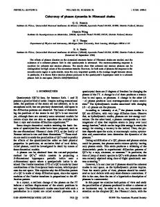
7.10 Round-trip delay distribution for packets from the Local server to USA . . . 72 7.11 Phase plot of round-trip delay for a packet interval of 1 ms . . . . . . . . . . 73 7.12 Phase plot of round trip delay for a packet interval of 100 ms . . . . . . . . . 73 v

7.13 Phase plot of round trip delay for a packet interval of 500 ms . . . . . . . . . 75 7.14 Round-trip delay plot emulated using NIST Net default parameters table for expected delay condition of 200 ms and std 7.07 ms . . . . . . . . . . . . . . 76 7.15 Round-trip delay plot emulated using measured Italy parameters table for expected delay condition of 200 ms and std 7.07 ms . . . . . . . . . . . . . . 76 7.16 Actual mean delay versus expected mean delay for 7.07 ms standard deviation 77 7.17 Actual standard deviation versus expected standard deviation for 100 ms, Italy acquired parameters table . . . . . . . . . . . . . . . . . . . . . . . . . . 78 7.18 Percentage of packets rejected at WS2 versus packet transmission rate . . . . 79 7.19 Phase plot of emulated round-trip delay for a packet transmission rate of 1000 Hz and input delay parameters of 200 ms mean delay and 14.14 ms standard deviation. . . . . . . . . . . . . . . . . . . . . . . . . . . . . . . . . . . . . . . 79 7.20 Phase plot of emulated round-trip delay for a packet transmission rate of 250 Hz and input delay parameters of 200 ms mean delay and 14.14 ms standard deviation. . . . . . . . . . . . . . . . . . . . . . . . . . . . . . . . . . . . . . . 80 7.21 Comparison of simulated versus emulated out of sequence packets for input delay condition of 100 ms mean delay and 7.07 ms standard deviation . . . . 80 8.1

Histogram of one-way time varying delay for 1000 Hz packet transmission rate using NIST net (a), and with data from the Italy experiment (b) . . . . 84

8.2

Histogram of one-way time varying delay for 500 Hz packet transmission rate using NIST Net (a), and with data from the Italy experiment (b) . . . . . . . 85

8.3

Histogram of one-way time varying delay for 100 Hz packet transmission rate using NIST Net (a), and with data from the Italy experiment (b) . . . . . . . 85

8.4

RMS position error between Cube 1 and Cube 2 for all the schemes using NIST Net (a), and with data from the Italy experiment (b) . . . . . . . . . . 87

8.5

Peak position error between Cube 1 and Cube 2 for all the schemes using NIST Net (a), and with data from the Italy experiment (b) . . . . . . . . . . 87

8.6

RMS force user applied to User 1 for all the schemes using NIST Net (a), and with data from the Italy experiment (b) . . . . . . . . . . . . . . . . . . . 88

8.7

RMS force user applied to User 2 for all the schemes using NIST Net (a), and with data from the Italy experiment (b) . . . . . . . . . . . . . . . . . . . 89

8.8

Comparison of out-of-sequence packets, and packets lost in transmission at WS1 . . . . . . . . . . . . . . . . . . . . . . . . . . . . . . . . . . . . . . . . . 90

9.1

Peer-to-peer scheme with wave variable delay compensation . . . . . . . . . . 95

9.2

Peer-to-peer scheme with time domain PO/PC delay compensation . . . . . . 96

9.3

(a), Histogram of one-way time varying delay (b), Time series plot . . . . . . 100

9.4

(a), Tracking of the cubes for wave variables (b), Wave variables . . . . . . . 100 vi

9.5

(a), Tracking of the cubes for TDP controller (b), PC action during the trial (c), The input and output energy at both user ends (d), Passivity control force applied to stabilize the system . . . . . . . . . . . . . . . . . . . . . . . 102

9.6

RMS position error between Cube 1 and Cube 2 measured at User 1 with parameter A . . . . . . . . . . . . . . . . . . . . . . . . . . . . . . . . . . . . 103

9.7

RMS position error between Cube 1 and Cube 2 measured at User 1 with parameter B . . . . . . . . . . . . . . . . . . . . . . . . . . . . . . . . . . . . . 103

9.8

Peak position error between Cube 1 and Cube 2 measured at User 1 with parameter A . . . . . . . . . . . . . . . . . . . . . . . . . . . . . . . . . . . . 104

9.9

Peak position error between Cube 1 and Cube 2 measured at User 1 with parameter B . . . . . . . . . . . . . . . . . . . . . . . . . . . . . . . . . . . . . 104

9.10 RMS Force rendered to User 1 with parameter A . . . . . . . . . . . . . . . . 105 9.11 RMS Force rendered to User 1 with parameter B . . . . . . . . . . . . . . . . 105 9.12 RMS Force rendered to User 2 with parameter A . . . . . . . . . . . . . . . . 105 9.13 RMS Force rendered to User 2 with parameter B . . . . . . . . . . . . . . . . 106 10.1 1-DOF target tracking with planar target on the side of the cube. . . . . . . . 111 10.2 Coordination task experiment with two users balancing a ball to stay within the specified boundary. . . . . . . . . . . . . . . . . . . . . . . . . . . . . . . . 113 A.1 Target tracking in Scheme 1 for 0 ms delay . . . . . . . . . . . . . . . . . . . 119 A.2 Force rendered to User 1 in Scheme 1 for 0 ms delay . . . . . . . . . . . . . . 120 A.3 Force rendered to User 2 in Scheme 1 for 0 ms delay . . . . . . . . . . . . . . 120 A.4 Target tracking in Scheme 1 for 0 ms delay . . . . . . . . . . . . . . . . . . . 121 A.5 Force rendered to User 1 in Scheme 1 for 200 ms delay . . . . . . . . . . . . . 121 A.6 Force rendered to User 2 in Scheme 1 for 200 ms delay . . . . . . . . . . . . . 122 A.7 Target tracking in Scheme 2 for 0 ms delay . . . . . . . . . . . . . . . . . . . 122 A.8 Force rendered to User 1 in Scheme 2 for 0 ms delay . . . . . . . . . . . . . . 123 A.9 Force rendered to User 2 in Scheme 2 for 0 ms delay . . . . . . . . . . . . . . 123 A.10 Target tracking in Scheme 2 for 200 ms delay . . . . . . . . . . . . . . . . . . 124 A.11 Force rendered to User 1 in Scheme 2 for 200 ms delay . . . . . . . . . . . . . 124 A.12 Force rendered to User 2 in Scheme 2 for 200 ms delay . . . . . . . . . . . . . 125 A.13 Target tracking in Scheme 3 for 0 ms delay . . . . . . . . . . . . . . . . . . . 126 A.14 Force rendered to User 1 in Scheme 3 for 0 ms delay . . . . . . . . . . . . . . 126 A.15 Force rendered to User 2 in Scheme 3 for 0 ms delay . . . . . . . . . . . . . . 127 A.16 Target tracking in Scheme 3 for 0 ms delay . . . . . . . . . . . . . . . . . . . 127 A.17 Force rendered to User 1 in Scheme 3 for 200 ms delay . . . . . . . . . . . . . 128 vii

A.18 Force rendered to User 2 in Scheme 3 for 200 ms delay . . . . . . . . . . . . . 129 A.19 RMS Position error between the target and cube 1 for three schemes . . . . . 129 A.20 RMS Position error between the target and cube 2 for three schemes . . . . . 130

viii

LIST OF TABLES Table Number

Page

3.1

Virtual coupling implementation issues . . . . . . . . . . . . . . . . . . . . . . 23

5.1 5.2

Virtual coupling parameters . . . . . . . . . . . . . . . . . . . . . . . . Two-factor design for the constant delay experiment. The 15 possible combinations are shown in numbers 1 - 15 . . . . . . . . . . . . . . . . Repeated-measures ANOVA summary (significant results only) . . . .

5.3 6.1 6.2 6.3 6.4 6.5 6.6

. . . . 38 trial . . . . 39 . . . . 43

Two-factor design for the Time-varying-delay experiment 1. The 12 possible trial combinations are shown in numbers 1 - 12 . . . . . . . . . . . . . . . . Three-factor design for the Time-varying-delay experiment 3. The 18 possible trial combinations are shown in numbers 1 - 18 . . . . . . . . . . . . . . . . Virtual coupling parameters . . . . . . . . . . . . . . . . . . . . . . . . . . . Delay condition with packet reflector location . . . . . . . . . . . . . . . . . Repeated-measures ANOVA summary for Experiments 1 and 2 (significant results only) . . . . . . . . . . . . . . . . . . . . . . . . . . . . . . . . . . . . Repeated-measures ANOVA summary for Experiment 3 (significant results only) . . . . . . . . . . . . . . . . . . . . . . . . . . . . . . . . . . . . . . . .

. 47 . 48 . 49 . 50 . 58 . 59

7.1 7.2

Emulator delay parameters input and expected round-trip characteristics . . 71 Average values from Internet delay characterization experiments . . . . . . . 74

8.1 8.2 8.3

NIST Net emulator delay parameters . . . . . . . . . . . . . . . . . . . . . . . 83 One-way emulated delay measured at WS1 . . . . . . . . . . . . . . . . . . . 86 Independent-samples t-test for all measures - significant results only . . . . . 89

9.1 9.2 9.3

Delay condition with packet reflector location . . . . . . . . . . . . . . . . Experiment parameters for time-delay compensation experiment . . . . . . Two-factor design for the time-delay compensation experiment. The 17 possible trial combinations are shown in numbers 1 - 17 . . . . . . . . . . . . . Paired-samples t-test - significant results only . . . . . . . . . . . . . . . . .

9.4

. 98 . 98 . 99 . 107

A.1 Test of Within Subjects Effects for Measure: RMSPE . . . . . . . . . . . . . 131 A.2 Pairwise Comparison Measure: RMSPE . . . . . . . . . . . . . . . . . . . . . 131 A.3 Test of Within Subjects Effects for Measure: PPSE . . . . . . . . . . . . . . . 132 ix

A.4 Pairwise Comparison Measure: PPSE . . . . . . . . . . . . . . . . . . . . . . 132 A.5 Test of Within Subjects Effects for Measure: RMSF1 . . . . . . . . . . . . . . 133 A.6 Pairwise Comparison Measure: RMSF1 . . . . . . . . . . . . . . . . . . . . . 133 A.7 Test of Within Subjects Effects for Measure: RMSF2 . . . . . . . . . . . . . . 133 A.8 Pairwise Comparison Measure: RMSF2 . . . . . . . . . . . . . . . . . . . . . 133 B.1 Test of Within Subjects Effects for Measure RMSPE From 1000 Hz Experiment134 B.2 Test of Within Subjects Effects for Measure PPSE From 1000 Hz Experiment 134 B.3 Test of Within Subjects Effects for Measure RMSF1 From 1000 Hz Experiment134 B.4 Test of Within Subjects Effects for Measure RMSF2 From 1000 Hz Experiment135 B.5 Test of Within Subjects Effects for Measure RMSPE From 500 Hz and 100 Hz Experiment . . . . . . . . . . . . . . . . . . . . . . . . . . . . . . . . . . . 135 B.6 Test of Within Subjects Effects for Measure PPSE From 500 Hz and 100 Hz Experiment . . . . . . . . . . . . . . . . . . . . . . . . . . . . . . . . . . . . . 135 B.7 Test of within Subjects Effects for Measure RMSF1 from 500 Hz and 100 Hz Experiment . . . . . . . . . . . . . . . . . . . . . . . . . . . . . . . . . . . . . 136 B.8 Test of Within Subjects Effects for Measure RMSF2 From 500 Hz and 100 Hz Experiment . . . . . . . . . . . . . . . . . . . . . . . . . . . . . . . . . . . 136 B.9 Pairwise Comparison of Schemes for Measure RMSPE from 1000 Hz Experiment . . . . . . . . . . . . . . . . . . . . . . . . . . . . . . . . . . . . . . . . 137 B.10 Pairwise Comparison of Delays for Measure RMSPE from 1000 Hz Experiment . . . . . . . . . . . . . . . . . . . . . . . . . . . . . . . . . . . . . . . . 137 B.11 Pairwise Comparison of Schemes for Measure PPSE from 1000 Hz Experiment . . . . . . . . . . . . . . . . . . . . . . . . . . . . . . . . . . . . . . . . 137 B.12 Pairwise Comparison of Delays for Measure PPSE from 1000 Hz Experiment 138 B.13 Pairwise Comparison of Schemes for Measure RMSPE from 500 Hz and 100 Hz Experiment . . . . . . . . . . . . . . . . . . . . . . . . . . . . . . . . . . . 138 B.14 Pairwise Comparison of Rates for Measure RMSPE from 500 Hz and 100 Hz Experiment . . . . . . . . . . . . . . . . . . . . . . . . . . . . . . . . . . . . . 138 B.15 Pairwise Comparison of Delays for Measure RMSPE from 500 Hz and 100 Hz Experiment . . . . . . . . . . . . . . . . . . . . . . . . . . . . . . . . . . . 139 B.16 Pairwise Comparison of Schemes for Measure PPSE from 500 Hz and 100 Hz Experiment . . . . . . . . . . . . . . . . . . . . . . . . . . . . . . . . . . . . . 139 B.17 Pairwise Comparison of Rates for Measure PPSE from 500 Hz and 100 Hz Experiment . . . . . . . . . . . . . . . . . . . . . . . . . . . . . . . . . . . . . 139 B.18 Pairwise Comparison of Delays for Measure PPSE from 500 Hz and 100 Hz Experiment . . . . . . . . . . . . . . . . . . . . . . . . . . . . . . . . . . . . . 140 x

B.19 Pairwise Comparison of Schemes for Measure RMSF1 from 500 Hz and 100 Hz Experiment . . . . . . . . . . . . . . . . . . . . . . . . . . . . . . . . . . B.20 Pairwise Comparison of Rates for Measure RMSF1 from 500 Hz and 100 Hz Experiment . . . . . . . . . . . . . . . . . . . . . . . . . . . . . . . . . . . . B.21 Pairwise Comparison of Delays for Measure RMSF1 from 500 Hz and 100 Hz Experiment . . . . . . . . . . . . . . . . . . . . . . . . . . . . . . . . . . . . B.22 Pairwise Comparison of Schemes for Measure RMSF2 from 500 Hz and 100 Hz Experiment . . . . . . . . . . . . . . . . . . . . . . . . . . . . . . . . . . B.23 Pairwise Comparison of Rates for Measure RMSF2 from 500 Hz and 100 Hz Experiment . . . . . . . . . . . . . . . . . . . . . . . . . . . . . . . . . . . . B.24 Pairwise Comparison of Delays for Measure RMSF2 from 500 Hz and 100 Hz Experiment . . . . . . . . . . . . . . . . . . . . . . . . . . . . . . . . . . . . B.25 Independent-samples t-test for measure RMSPE . . . . . . . . . . . . . . . B.26 Independent-samples t-test for measure PPSE . . . . . . . . . . . . . . . . . B.27 Independent-samples t-test for measure RMSF1 . . . . . . . . . . . . . . . . B.28 Independent-samples t-test for measure RMSF2 . . . . . . . . . . . . . . . .

. 143 . 144 . 145 . 146 . 147

C.1 C.2 C.3 C.4 C.5 C.6 C.7 C.8

. . . . . . . .

Test of Within-Subjects Effects for Measure: RMSPE Pairwise Comparison Measure: RMSPE . . . . . . . . Test of Within-Subjects Effects for Measure: PPSE . . Pairwise Comparison Measure: RMSPE . . . . . . . . Test of Within-Subjects Effects for Measure: RMSF1 . Pairwise Comparison Measure: RMSF1 . . . . . . . . Test of Within-Subjects Effects for Measure: RMSF2 . Pairwise Comparison Measure: RMSF2 . . . . . . . .

xi

. . . . . . . .

. . . . . . . .

. . . . . . . .

. . . . . . . .

. . . . . . . .

. . . . . . . .

. . . . . . . .

. . . . . . . .

. . . . . . . .

. . . . . . . .

. . . . . . . .

. . . . . . . .

. 141 . 141 . 141 . 142 . 143

148 149 150 151 152 153 154 155

GLOSSARY Networked Haptic Virtual Environment.

NHVE:

RMS:

Root Mean Square.

DOF:

Degrees of Freedom.

UDP:

User Datagram Protocal

TCP:

Transmission Control Protocal

3D:

Three Dimensional

GUI:

Graphical User Interface

HCOLGUI:

Haptic Collaboration Graphical User Interface

HC:

Haptic Controller

HO:

Human Operator

QOS:

Quality of Service

DC:

Direct Current

RMSPE:

PPSE:

Root Mean Square Position Error

Peak Position Error

RMSF1:

Root Mean Square Force Appplied to User 1 xii

RMSF2:

Root Mean Square Force Appplied to User 2

xiii

ACKNOWLEDGMENTS

I would like to express my sincere appreciation and gratitude to Dr. Blake Hannaford for his constant guidance, patience and motivation. His helpful nature, both academic and personal, have helped in easing my anxiety and allowed me to feel at home here. His ability to pierce through a problem simply amazes me. I am truly honored to have worked with him. I thank my committee members Dr. Steven Venema, Dr. Howard Chizeck and Dr. Eric Klavins for their guidance with my thesis work. Especially I want to thank Dr. Steven Venema for tirelessly going over several drafts of this thesis even with his busy schedule at the Boeing Company and Dr. Howard Chizeck on many valuable comments and insights during our weekly teleoperation meetings. I also want to thank Dr. Jim Troy, Dr. Kevin Puterbaugh and Dr. Steven Venema from Boeing Company for many of the initial discussions that lead to this thesis. This work could not have been possible without our collaborators who hosted the packet reflectors in their server. I want to thank, Dr. Tim Salcudean and Orcun Goskel from University of British Columbia, Canada, Dr. Oliver Tonet from Scuola Superiore Sant’Anna, Italy and Krish Karthik from North Carolina State University, USA for hosting the packet reflector network in their servers. I also want to thank all the members of the bioRobotics Laboratory for the great time I had during the course of this study. It is such a great place to work and I am glad I chose to come here to work on my PhD. I am truly going to miss them. I thank my wife Sol for being so kind and understanding during the final stages of my work. Her constant encouragement, tireless proofreading of this thesis have helped me tremendously. Its due to her strength and fortitude that I was able to invest the time and effort needed to complete this thesis work. xiv

I thank my parents for the sacrifices they have made to assist me during my studies here. I am truly indebted to them. Their love and affection from thousands of miles away have given me the much needed strength in pursuing my goals. Finally, I thank the Almighty, Lord Muruga for answering my prayers and giving me true wisdom.

xv

DEDICATION To my parents Sankaranarayanan and Saraswathy and to my wife Sol Vedovato.

xvi

1

Chapter 1 INTRODUCTION

As humans we are social creatures, interacting through speech, touch and vision. For instance, the experience of holding a piece of a particular rock in hand and learning about it gives far greater wisdom than learning about it through books. Moreover, we all learned to write by either our parents or the teachers holding our hands and guiding us to complete the alphabet. As an example, the task of windshield placement for a car is shown in Fig. 1.1. Here the two persons collaborate in the task by distributing the weight of the windshield and then maneuvering it to the right place to be fitted permanently. In this situation, one person could be a trainee and the other, an instructor teaching the process of installing the windshield. Visual, auditory and tactile cues are all used to complete the task. Modern day computers have evolved to be a single user interface, which greatly hinders our natural interaction process[1]. Nevertheless, they also have enormous computing power compared to systems just a decade ago; and even an off-the-shelf graphics card is capable of producing computer graphic scenes with moderate complexities, a far cry from the line drawings that early computers used to render. Internet connectivity is getting better and cheaper each day. These developments have spurred the growth of networked virtual environment (NVE) applications such as multiplayer games and interactive 3D virtual worlds were multiple users interact using avatars (Fig. 1.2). In [1], they cite an example of a street in foreign city that one could visit in this virtual space to converse with the local people and learn their native language. Virtual reality systems like CAVE [2] have been developed to give the users a complete immersive environment that mimics day-to-day natural interaction. Such systems also allow multiple users to share the same virtual space thereby enabling interaction among them. For example, in the windshield installation task, two users could interact in the virtual

2

Figure 1.1: Two persons collaborating to install a windshield in a car.

Figure 1.2: Screen shot from Active Worlds application showing people interacting with avatars in a NVE.

3

Figure 1.3: Typical CAD assembly environment in aerospace industry.

space holding a virtual windshield and placing it on a virtual car. With computer aided design (CAD) used in all manufacturing processes, a computer graphic model of the various manufacturing parts could be added in a virtual space which then could be used for making design decisions, and training of parts assembly tasks and maintenance tasks. An example of a CAD model from the aerospace industry is shown in Fig. 1.3. Haptics is an important sensory mode that has been lacking in many of the virtual reality systems. Virtual reality systems with haptic feedback could be in military training [3], surgery training [4], CAD assembly [5], virtual sculpting [6] and haptic painting, [7] among other applications. Many of these applications require collaboration among multiple users. For example, in a CAD assembly task, the experts might not be in the same location and they might have to connect to the virtual environment by a dedicated network or the Internet. This is increasingly true in today’s globalized manufacturing environment. A Networked Haptic Virtual Environment(NHVE) is an important necessity in such applications. Moreover, NHVEs have the potential to bring realistic force feedback to multi-player networked games, thereby vastly enhancing their realism. NHVEs are implemented as either peer-to-peer (distributed) or client-server (centralized) architectures using either a dedicated network or the Internet. Since NHVEs have a wide range of applications, the implementation of such systems poses several challenges. For

4

Figure 1.4: Relationship between mobility/error tolerance and force in a NHVE.

Figure 1.5: Relationship between bandwidth and delay in a NHVE.

5

Figure 1.6: Relationship between dexterity and computational complexity/DOF in a NHVE.

example, in gaming applications, the ability of users to move quickly and interact with virtual objects is more important, compared to CAD assembly tasks where importance is given to maintaining very low position errors between the copies of the virtual objects that the users share. In general, depending on the type of NHVE application, the design specifications for a NHVE includes: • Delay and bandwidth • Error tolerance • Force range • Mobility • Dexterity • DOF

6

• Computational complexity Figs. 1.4, 1.5 and 1.6 show the relationship among different design specifications based on three chosen applications, namely surgery training, virtual assembly training and entertainment/gaming. Fig. 1.4 shows a plot of mobility/error tolerance versus force range for a NHVE. Here the error tolerance refers to the magnitude of error between the copies of the virtual objects that the users share in a NHVE that is acceptable for a given application. Mobility is the ability of the users to move the virtual object in the NHVE. For the surgery training application, very low error tolerance is required and applications such as CAD virtual assembly task a low to medium error tolerance is required since any position drift between the copies of the virtual object would make the collaboration meaningless after certain time. Entertainment/gaming applications usually can tolerate larger position errors but mobility is crucial for them. In surgery and virtual assembly tasks, the mobility requirements usually ranges from low to medium respectively. Fig. 1.5 shows a plot of bandwidth versus delay for a NHVE. The delay is characterized as local, regional, and global corresponding to local area network (LAN), wide area network (WAN) with single backbone and WAN with multiple backbone networks. All three applications may be operated in all the delay conditions whereas entertainment/gaming applications usually occupy less bandwidth than surgery training or virtual assembly tasks. In addition, the latter might require medium to high bandwidth because of the high update rate of 1000 Hz required to feel stiffer objects, such as metal parts [8]. Fig. 1.6 shows a plot of dexterity versus computational complexity/DOF for a NHVE. The DOF refers to number of degrees of freedom of force feedback available to users in NHVE. Devices with more DOFs are also expensive. For entertainment/gaming applications, usually the force feedback is limited to one to two DOFs whereas in surgery training and virtual assembly tasks three to six DOFs are often required. High dexterity is required for the surgery training and virtual assembly tasks compared to low dexterity required for entertainment/gaming applications as well. Apart from these design specifications, a NHVE system should be guaranteed to remain stable during the entire duration of the collaboration. This is particularly important since

7

bilateral systems —in which energy flows in both directions— like those in NHVEs tend to quickly destabilize in the presence of time delays. Moreover in collaboration using networks such as Internet the system should also be resilient against delay variations (jitter) and loss of communication packets since this can adversely affect the stability of the system. 1.1

Focus of This Thesis

This thesis focuses on implementation of NHVEs that require low error tolerance such as for virtual assembly tasks and surgery training. It presents three different virtual coupling schemes, one using client-server and two using peer-to-peer architectures for maintaining position coherency among the copies of virtual objects in a NHVE. A client-server architecture with a central server which manages one copy of the virtual object is efficient in maintaining position coherency, but round-trip delay is added between the clients and the server. In contrast, in a peer-to-peer architecture, each peer maintains a copy of the virtual object and updates it locally. Therefore, this architecture has half the delay of the client-server architecture but is more susceptible to position discrepancy among the virtual objects. Hence the two peer-to-peer virtual coupling schemes are compared to a client-server based virtual coupling scheme in terms of how well they minimize the error between the positions of the virtual copy of the rigid body that multiple users share in a NHVE, as well as in terms of force, target tracking error, and other measures of performance. 1.1.1

Position Coherency

We define position coherency in a NHVE as the position discrepancy between the multiple copies of a virtual object at a single instant of global time. 1.2

Organization of the Thesis

This document is organized as follows: The Introduction chapter gives a brief overview of the research area and its problems, followed by the Background chapter, in which previous literature in this area is classified and explained. The motivation for introducing the schemes in terms of general collaboration setup is given in the Virtual Coupling Schemes chapter, and the three virtual coupling schemes are explained in detail. Subsequently, the

8

Experimental Collaborative Haptic System chapter expounds the experimental setup and procedure for the experiments, while the Constant Delay Experiments chapter presents a comprehensive explanation of the results from testing the virtual coupling schemes for constant time delay. The sixth chapter, Experimental Internet Haptic Collaboration using Virtual Coupling Schemes thoroughly explains the results from the global scale Internet haptic collaboration experiment using these virtual coupling schemes. In the Time Varying Network Delay and Characterization chapter, the experiments to characterize the Internet and emulation of similar characteristics in a laboratory setting are presented followed by the analysis of their performances in the chapter named Comparison of Performance of Virtual Coupling Schemes for Haptic Collaboration using Real and Emulated Internet Connections. Additionally, in Experimental Comparison of Internet Haptic Collaboration with Time-Delay Compensation Techniques, the performance of two time-delay compensation techniques and a tuned PD controller applied to one of the virtual coupling scheme was compared. The final chapter presents the conclusion and future work.

9

Chapter 2 BACKGROUND

It has been shown in [9, 10, 11] that the inclusion of haptics in a shared virtual environment increased the task performance and virtual presence felt by the users. The general scheme of testing used in these methods is shown in Fig. 2.1. The experiments consist of two display monitors and two haptic devices connected to a single computer. The second monitor and the haptic device are usually kept in a separate room connected by a long cable to the computer. In [11], there were five tasks comprised of jointly manipulating a set of cubes inside a virtual environment. The experiment was evaluated using a questionnaire. There were no time delays between the two users. In [10], a simple game called “ring on a wire” was used: In this game two users collaborate to thread a ring along a wire between two ends. The effectiveness of the collaboration was determined using the number of times the users make contact with the wire as they move the ring along the wire. In [12], the inclusion of network delays in a cooperative shared haptic virtual environment was found to reduce the task performance. Time delay in a closed loop system poses a serious problem by driving the system unstable. For example, teleoperation has been studied extensively and it has been shown that feedback delays in excess of one-third of a second become troublesome for the operator [13, 14, 15]. Bilateral teleoperation —in which forces are fed back to the master to enable the sense of touch and feel of the remote environment– requires the transmission of forces from DC to very high frequency to enable the operator to feel the normal and tangential forces. For larger delays, feedback bandwidth is either limited to very low frequencies or energy dissipating elements are added in the system making the device feel very sticky and difficult to operate. Previous work in NHVEs can be classified based on the type of control used as either a centralized (client-server) [16, 17, 18, 19, 20] or a distributed (peer-to-peer) architecture

10

Display 1

Room 1

Haptic device 1

Room 2

Display 2

Haptic device 2

Host Computer

Figure 2.1: Shared virtual environment with dual displays

[21, 22, 23, 24]. Based on the type of force rendering, NHVEs can be further classified into simultaneous [17, 18, 19, 23, 25, 24, 26], where the users manipulate a virtual object at the same time, and one-at-a-time [21, 22, 16], where each user takes turns in manipulating the virtual object.

2.1

Centralized or Client-server Architecture

The centralized architecture as shown in Fig. 2.2 consists of a central server to which multiple clients establish connection. Each client could be at a different location and would generally have different time delays in communicating with the server. The server maintains the status of the virtual objects that the clients share and manipulate. Each client interacts with these virtual objects using a haptic device, whose position is sent to the server usually at the same rate as the local servo loop. The server usually buffers the position input in order to use inputs from all the clients as a single net input. Collision detection between the position inputs of the multiple clients and the virtual objects is performed at the server and the position of the virtual objects is updated. The new position of the virtual objects is then transmitted back to clients for updating at their local computer. Each client uses this updated position locally to compute forces to be transmitted to the haptic device. The advantages of this architecture are:

11

Server Client 1 Client n Client 2

Client 3

Figure 2.2: Client-Server Architecture

• Since the position of the virtual objects is maintained and updated at the server as a single virtual environment model, there are no coherency discrepancies. • Clients can join or leave the simulation at any time. • Virtual objects can be added or deleted easily during the simulation. • By buffering the client inputs, fairness among clients having different delays is achieved. The disadvantages of client-server architecture include: • Each client experiences a round-trip time delay before their copy of virtual object is updated from the server. • By employing a buffering scheme, the clients nearer to server have to unnecessarily experience larger delays. • The connection to the server has to be maintained at all times to continue the simulation.

2.2

Distributed or Peer-to-peer Architecture

A simple peer-to-peer architecture is shown in Fig. 2.3. It consists of a network connecting multiple clients, each running their own simulation with copies of the virtual environment.

12

Client 1

Client 2

Client 3

Client n

Figure 2.3: Peer-to-Peer Architecture

Each client also uses the haptic device for input and output. During the simulation, each client multicasts its position information to all other clients. The clients then individually perform collision detection and update the position of the local copy of the virtual object and render appropriate forces. The advantages of this architecture are: • There is less delay compared to the client-server architecture since each client multicasts information to all other clients. • Since virtual objects are updated locally, the reaction to each client input is reflected immediately. The disadvantages of this architecture are: • Because of the distributed nature of the simulation, the coherency between the copies of the virtual object among the clients is not guaranteed. • It is often difficult to add or remove new clients during the simulation. 2.3

Previous Work with One-at-a-time Force Rendering Techniques

In [21], a haptic collaboration system over the Internet was developed introducing both static (anchored) and dynamic (movable) objects in their collaboration setup. The object database had information about all of the objects in the environment and the node database had information about the IP addresses, latency, and available bandwidth. The nodes that

13

had high bandwidth and low latency multicasted the position and orientation of the objects they own, whereas the nodes with high latency became passive observers. Forces felt by the users were as if they were the only ones interacting with the objects. In [22] a force feedback, multiplayer squash game was implemented using a peer-to-peer architecture on the Internet. An adaptive-dynamic bounder algorithm was used to restrict the maximum change in speed after the collision of the ball with a virtual object. A multi-user heterogeneous system was implemented in [16], which had a single object that each user manipulated. Each user got a short amount of time to manipulate the object and generate reaction forces, and perceived this environment as though all the users simultaneously manipulated the object. 2.4

Previous Work with Simultaneous Force Rendering Techniques

A two-user transatlantic distributed collaboration system was implemented in [23], whose emphasis was on evaluating virtual presence in the presence of large latency with jitter. Two users collaborated in the simple task of moving a cube up from the floor. Force applied by each user at their end was transmitted instead of position, and damping was added to the system at all contacts to make it stable. The virtual presence was evaluated using a questionnaire, which showed that collaboration is still possible in a system with large latency. In [26] a multi-rate control architecture for haptic collaboration was proposed and the stability and performance was studied for a fixed transmission rate of 128 Hz and with small communication latency. In [27], a peer-to-peer system with local and global representation of the virtual objects was used for collaboration. TCP/IP was used for communication at low packet transmission rates and locally an optimistic simulation predicted the position of the virtual objects until new information was updated through the network. The simulation was stopped if there were any large discrepancies in position of the local and global representations. 2.5

Media Synchronization Techniques

Attempts have also been made to implement media synchronization techniques available in video and audio streaming [28] for haptic media. The haptic media synchronization

14

consists of intra-stream, inter-stream, and group(or inter-destination) control. The intrastream media synchronization is used to preserve the timing information among the media units in a single media stream, while the inter-stream media synchronization is used in preserving temporal relationship among multiple media streams. Group synchronization control is used to adjust the output timing of the media streams from multiple clients to enforce fairness among them. A queue monitoring (QM) algorithm was used in [17] for intra-media synchronization of haptic media between a single client and a server. They also used dead reckoning for traffic control of haptic media. They showed improvement in their system with media synchronization using a subjective score of operationality. In [18] a temporal resolution control of haptic media by dynamically changing the output rate of the haptic media was implemented. Group synchronization control for haptic media was implemented in [19]. They used a synchronization “maestro” to adjust the output timing of the haptic media among multiple clients.

15

Chapter 3 VIRTUAL COUPLING SCHEMES 3.1

Motivation

Time delay has been a well known problem in teleoperation. Much work [29, 30, 31, 32, 33, 34, 35, 36, 37, 38, 39, 40, 41, 42] has been done in this area for maintaining stability in the presence of time delays. One might think that, if we could pose the NHVE problem similar to bilateral teleoperation, there would be several methods that could be readily available for maintaining stability in terms of time delays as well as position control of the virtual objects. An attempt will be made in this thesis to integrate NHVEs into an overall collaboration network of which bilateral teleoperation is a also a subpart. The collaboration framework is explained in the subsequent section. 3.2

General Collaboration Framework

The general collaboration framework is shown in Fig. 3.1. It consists of a computer network connecting multiple mechanical devices, which could be active or passive based on the type and application. These devices could interact with virtual or real environments and could be driven by a human operator or coupled to another device. Several interesting subsets of collaboration could be derived from this generalized diagram. To better understand the system, a simplified block diagram representing two haptic devices is shown in Fig. 3.2. Blocks B and G represent haptic devices 1 and 2. Blocks C and F represent the system or controller that the devices are connected to. The virtual environments that the haptic devices interact with are represented in blocks D and E. The human operator and the real environment are represented in blocks A and H respectively. Several interesting subsets that could be derived from the block diagram representation are:

16

• Blocks ABCFGH represent a bilateral teleoperation. Block H could be either HO or Environment.

• Blocks ABCD represent a single user interacting with the virtual environment. • Blocks ABCDEFGH represent a two-user haptic collaboration using a shared virtual environment.

• Blocks ABCDFGH represent a two-user collaboration with a single virtual environment. The subset that will be focus of this thesis is block ABCDEFGH. 3.3

Virtual Coupling Schemes

A virtual coupling is a simulated physical connection between the haptic device and the virtual environment. It may provide stable interaction regardless of the complexity of the virtual environment or the level of human grasp interaction. Such a coupling was first proposed by [43] and a similar god-object method was used in [8]. Furthermore, in [44], a two-port network was used to analyze virtual coupling schemes for both impedance and admittance type of haptic devices. In this work, an impedance-type virtual coupling is used to connect the haptic device and the virtual copies of the rigid bodies that are shared in the NHVE. Depending on the type of NHVE —either peer-to-peer or client-server— additional virtual couplings are proposed to couple the remote users haptic handle positions to the local copy of the rigid body and to track multiple copies of the rigid bodies. Based on the type of virtual coupling connections, two peer-to-peer virtual coupling schemes are proposed, one with a virtual coupling between the copies of the rigid body and the other that couples remote users haptic handle positions locally for each peer. Additionally, a virtual coupling scheme is proposed for the client-server architecture, where each client’s haptic handle positions are coupled to the rigid bodies maintained at the server using virtual couplings. A local virtual

17

HO1

HOi

MECH

MECH

COMPUTER NETWORK

VE1

MECH

REAL ENVIRONMENT

Figure 3.1: General schematic

MECH

18

D

E VE1

VE2

T

C

C1

C2

F

T

B

G HD1

HD2

A HO

Environment

H

Figure 3.2: General collaboration framework

coupling is used to render forces for each client, which provides them with undelayed force responses. Apart from the three schemes proposed in this work, two additional virtual coupling schemes —one representing a peer-to-peer and the other a client-server architecture as proposed in [26]— are also described; their advantages and disadvantages are compared to the virtual coupling schemes presented in this work.

3.3.1

Virtual Coupling Scheme 1

This two-user, one degree of freedom, simplified collaboration model is shown in Figs. 3.3, 3.4 and 3.5 for VC schemes 1-3 respectively. In this simplified model, the human operator input is position while reaction force is the output. A virtual copy of the position of the haptic devices in the collaboration environment is represented by the haptic handles H1−1 and H2−2 . The virtual copies of the rigid body that users manipulate are represented by O1−1 and O1−2 . KV C1 , BV C1 , KV C2 and BV C2 represent virtual couplings that transmit forces to users 1 and 2, respectively. The position of the haptic devices are x1 and x4 and the virtual copies of the rigid bodies are x2 and x3 . Collision detection between the user

19

Figure 3.3: Virtual coupling scheme 1

position input and the rigid body was computed using a bounding box method. The Figs. 3.3 and 3.4 represent the control structure in a peer-to-peer architecture. Fig. 3.5 represents the control structure in a client-server architecture. The objective of all three methods is to minimize the position error between x2 and x3 . The dotted lines separate the local and the remote user that are connected by a communication network. The communication latency between a client and the server and between peers are represented by delays T1 (t) for the communication path left to right and T2 (t) for the path right to left respectively.

F1 = KV C1 (x2 (t) − x1 (t)) + BV C1 (x˙2 (t) − x˙1 (t)) m x¨2 (t) = KT (x3 (t − T2 (t)) − x2 (t)) 2 +BT (x˙3 (t − T2 (t)) − x˙2 (t)) − F1 − Bd x˙2 (t) F2 = KV C2 (x3 (t) − x4 (t)) + BV C2 (x˙3 (t) − x˙4 (t)) m x¨3 (t) = KT (x2 (t − T1 (t)) − x3 (t)) 2 +BT (x˙2 (t − T1 (t)) − x˙3 (t)) − F2 − Bd x˙3 (t)

(3.1)

(3.2) (3.3)

(3.4)

In Scheme 1 (Fig.3.3), a direct virtual coupling is applied between two copies of the rigid body, each having half of the mass. This enables the two virtual copies of the masses to track each other and also to transmit forces between them. This approach is highly reminiscent of the PD controller in bilateral teleoperation [35]. In order for the total mass felt by the user

20


to be consistent, they are equally divided among the two users virtual copies. The virtual coupling between the masses is implemented using a position-position architecture through the simulated communication link. The reaction force applied to Users 1 and 2 is computed using the local virtual coupling and it is given in equations 3.1 and 3.3. The force acting on each user’s copy of the rigid body depends on the user’s position input at the local end and also the position difference between the rigid bodies. Viscous damping Bd is added between the cube and the surface to keep the mass from drifting off when users were not in contact. Equations 3.2 and 3.4 describe the force acting on each user’s copy of the rigid body. 3.3.2


Scheme 2 (fig. 3.4) represents a parallel control structure where each user manipulates the rigid body at his own end. Position input of the haptic device is coupled to the rigid body through a local virtual coupling. Forces are applied to each copy of the mass by a virtual coupling, one for each user. The equations describing Scheme 2 are:

F1 = KV C1 (x2 (t) − x1 (t)) + BV C1 (x˙2 (t) − x˙1 (t))

(3.5)

mx¨2 (t) = KV C21 (x4 (t − T2 (t)) − x2 (t)) +BV C21 (x˙4 (t − T2 (t)) − x˙2 (t)) − F1 − Bd x˙2 (t) F2 = KV C2 (x3 (t) − x4 (t)) + BV C2 (x˙3 (t) − x˙4 (t))

(3.6) (3.7)

21


mx¨3 (t) = KV C12 (x1 (t − T1 (t)) − x3 (t)) +BV C12 (x˙1 (t − T1 (t)) − x˙3 (t)) − F2 − Bd x˙3 (t) 3.3.3

(3.8)


Scheme 3 (Fig. 3.5) represents the client-server architecture where User 1 is on the server and User 2 is in the client. There is only one copy of the rigid body which is in the server. User 2’s position is transmitted to the server where the position of the rigid body is updated. The updated position of the rigid body is then transmitted to the User 2 and it is used to compute local forces using the virtual coupling KV C2 and BV C2 . In this scheme, User 1’s position is not delayed since User 1 is in the server. The equations describing Scheme 3 are:


(3.9)

mx¨2 (t) = KV C21 (x4 (t − T2 (t)) − x2 (t)) +BV C21 (x˙4 (t − T2 (t)) − x˙2 (t)) − F1 − Bd x˙2 (t)

(3.10)

x3 (t) = x2 (t − T1 (t))

(3.11)


(3.12)

22

3.4

Virtual Coupling Schemes Implementation Issues

In order to implement the three virtual coupling schemes, several factors need to be taken into account. First, the number of virtual couplings needed for each schemes varies and moreover for a 6-DOF implementation, twice the number of virtual couplings required for a 3-DOF are needed. With large number of users, managing and computing reaction forces would become cumbersome. The number of collision detections between the user’s haptic handle and the rigid body for each user needs to be minimum since many of the NHVEs will have complex scenes and collision routines are computationally expensive. Moreover, in Scheme 1 the mass of the virtual object is divided equally among the copies of the rigid body that the users share in a NHVE. For predetermined number of users, the implementation of Scheme 1 does not pose any problem. If for some reason a new user needs to be added in the middle of the collaboration, the the mass of the virtual object needs to be redistributed among the new number of copies of the virtual object. Redistributing the mass on the fly may seriously affect the stability and performance of the system. The collaboration may need to be stopped and restarted later after adding the new users and making necessary changes. Table 3.1 summarizes the implementation issues for the virtual coupling schemes in terms of number of virtual couplings and collision detection. It can be seen that Scheme 1 requires the lowest number of collision detection among the three schemes. Moreover, for more than three users, Scheme 3 requires a lesser number of virtual couplings compared to Schemes 1 and 2.

3.5

Comparison to Other Virtual Coupling Schemes

In [26], two virtual coupling schemes one representing peer-to-peer and the other a clientserver architecture was proposed. In this section the difference between their virtual coupling schemes and the ones proposed in this work are described.

23

Table 3.1: Virtual coupling implementation issues

3.5.1

Virtual coupling

No.

of virtual

schemes

couplings

No.

of collision

detections

3 DOF

6 DOF

User

Total

1

n(n+1) 2

n(n + 1)

1

n

2

n2

2n2

n

n2

3

2n

4n

1

2n

Comparison of the Peer-to-peer Virtual Coupling Schemes

A two-user peer-to-peer virtual coupling scheme as proposed in [26] is shown in Fig. 3.6. This scheme is a combination of Schemes 1 and 2 proposed in this work. In addition to the direct virtual coupling between the two copies of the rigid bodies, the user’s haptic handle positions are also coupled to the rigid body through a local virtual coupling. In this architecture, the mass of the rigid body was not equally divided among its multiple copies. Even under no communication delay, the mass of the rigid body felt by the users would be higher than the actual mass. Moreover, in terms of implementation, the number of virtual couplings and collision detections required for this method is more than that required for implementing either Scheme 1 or 2.

3.6

Comparison of the Client-server Virtual Coupling Schemes

A two-user client-server virtual coupling scheme as proposed in [26]is shown in Fig. 3.7. This scheme is similar to the Virtual coupling scheme 3 proposed in this work except that each client’s force feedback is computed at the server. Under zero communication delay, there is no difference between the two virtual coupling schemes. However, in the presence

24

Figure 3.6: Peer-to-peer virtual coupling scheme

Figure 3.7: Client-server virtual coupling scheme

of communication delays, the delayed force feedback to the clients from the server would allow each client to penetrate deeper into the rigid body, thereby making it unstable. In Scheme 3, a local virtual coupling provides immediate force feedback for each client using the most updated position of the rigid body received from the server. This local virtual coupling prevents clients from penetrating deeper into the rigid body in the presence of communication delay. Therefore, Scheme 3 could be used under arbitrary communication delays whereas the client-server scheme[26] cannot be used under communication delays without considerably reducing the impedances of the virtual couplings.

25

Chapter 4 EXPERIMENTAL COLLABORATIVE HAPTIC SYSTEM

In this chapter, I explain in detail the experimental collaborative haptic system built to test the virtual coupling schemes under constant and time-varying network delay conditions. The experimental collaborative haptic system consists of a collaboration software framework that implements the peer-to-peer and client-server NHVE system, collaboration hardware setup, and a network packet reflector setup which enables experiments using the Internet. 4.1

Collaboration Software Framework

The collaboration software framework is shown in Fig. 4.1. There are two separate programs for each user. The Haptic controller program (written in C++) manages communication with the haptic device, performs collision detection and dynamic updates of the virtual object, renders the appropriate forces to the user, and performs haptic UDP communications at variable rates. The graphical display is managed separately by the HColGUI, an application based on Qt 4.1.1.1 and OpenGL libraries.

4.1.1

Haptic Controller

The haptic controller program consists of a main process in which all the application threads are managed. The haptic process —which runs on a separate thread at 1000 Hz— manages communication to the haptic device and updates the collision and virtual coupling forces to the virtual object. The communication to other peers or a server and to the HColGUI are managed via TCP and UDP socket handlers. A collaboration database containing peer/server information is maintained in the haptic controller whose values are all loaded as a configuration file at the beginning of the collaboration. Whenever new information from another peer/server is available at the UDP socket,

26

Figure 4.1: Haptic collaboration software architecture

27

the UDP packet handler function is called by the UDP callback function, where the UDP packet information is processed for update of the peer/server information. Each UDP haptic data packet has a unique packet sequence number generated in the haptic servo loop and a checksum field generated using a simple checksum algorithm. This information is used by the UDP packet handler function to detect corrupt and out-of-sequence packets. For this work, both the corrupt and out-of-sequence packets were dropped and the last valid packet information was utilized until the information is updated; essentially, a zero-order hold (ZOH). The haptic data packets also contain a time stamp field that is applied to compute the network delay characteristics. The valid UDP haptic data from peers/server is then passed to the haptic process in a thread safe manner for force and position updates. The new information for other peers/server is sent from within the haptic process by the packet transmission rate controller function, where the packet transmission rate is precisely controlled by the haptic servo loop. The structure of the UDP haptic data packet is shown below: typedef struct{ unsigned long int servoTick; /* servo loop number */ RtUTCtime p_timestamp; /* peer timestamp */ double g_pos[3]; /* Goal position - Scheme 3 (HIP) */ double c_pos[3]; /* Constraint position - Scheme 2 (IHIP) */ double g_rb[3]; /* Rigid Body Position- Scheme 1*/ double v_rb[3]; /* Rigid Body Velocity - Scheme 1*/ double t_pos[3]; /* Haptic handle velocity - Scheme 2*/ int checksum; }udpPeerData; The event-based TCP/IP communication between the HColGUI and the haptic controller is modeled as a client/server communication with the TCP server running on the haptic controller and the HColGUI acting as a client. The TCP/IP communication from HColGUI is processed by the TCP callback function which in turn calls the TCP packet handler function. The collaboration commands are then enabled through the haptic device

28

interface function that facilitates communication to and from the haptic device at run-time. The peer information received from the TCP packet handler on TCP port 12346 is used to update the local peer database. The same TCP port is also used to exchange tracking information between peers, as explained later in the experiment procedure. The structure of the TCP communication packet is shown below; it consists of integer field containing a secret code for security that is verified before establishing a connection. The deviceAttach field is used to attach the haptic device for the collaboration, while the deviceNum field is for future use to support multiple haptic devices, and the gO field is used to start and stop the collaboration and the tracking field is used to initiate tracking during the collaboration. typedef struct{ int secret; /* secret code */ int deviceAttach; /* Attach specified haptic device */ int deviceNum; /* Haptic device number */ int gO; /* Start collaboration */ int tracking; /* Start target tracking */ }tcpGUI2HC; The graphic display updates from the haptic controller to the HColGUI are done at a rate of 30 Hz using a TCP/IP communication link on TCP port 12345. Whenever new graphic updates need to be sent to the HColGUI, the haptic thread is locked and all information is copied in a synchronous manner to the HColGUI. For the current implementation, the synchronous thread option provided by the OpenHaptics Toolkit is used to copy haptic data in a thread safe manner. The TCP packet structure for graphic display updated is given below: it consists of two position fields that represent the goal position of the haptic probe of the Users 1 and 2 and two position fields that represent the constraint position of the haptic probe of the same users. It also contains a field for the tracker position, which is currently unused, and a field for the position of the rigid body that is used in the collaboration. The integer fields fcolor2 and tracking holds the information about the current display color for the virtual object and the target. typedef struct{

29

double g_pos1[3]; /* User 1 goal position (HIP) */ double g_pos2[3]; /* User 2 goal position (HIP) */ double c_pos1[3]; /* User 1 constraint position (IHIP) */ double c_pos2[3]; /* User 2 constraint position (IHIP) */ double t_pos[3];

/* Target position*/

double position_rb[3]; /* Rigid body position */ int fcolor2; /* Rigid body color */ int tracking; /* Target color */ }tcpHC2GUI;

4.1.2

HColGUI

The graphics app HColGUI gets display updates from the haptic controller through a TCP/IP connection at 30 Hz. The Qt OpenGL Widget interface is used to graphically render the position of the virtual object and the positions of the local and remote users. The HColGUI also has two menu interfaces: the server connection dialog and the peer dialog. The server connection dialog is used by each peer/client to connect to their local haptic controller. This dialog is also used to choose a specific haptic device for collaboration and opt to start and stop the collaboration. The peer dialog is used for managing peers/clients connections. For example —in a peer-to-peer collaboration— the peer that is initiating the collaboration would start a TCP server on port 12346, followed by the other peers connecting to it for collaboration. Figure 4.2 shows the snapshot of the haptic virtual environment as seen by User 1. It consists of a cube that is restricted to one-degree-of-freedom movement on a floor in a threedimensional room. The local and remote user positions are represented by blue and yellow spheres respectively. The haptic virtual environment also contains a target sphere that moves at a constant speed along a solid white line. The task of the users is to jointly move the cube along the line and to make the target align at the center of the cube at all times. The users can feel all the sides of the cube but can contribute to motion only by pressing on the left or right side of the cube. In this work, User 1 was allowed to touch the left side of

30

Target sphere

User 1

User 2

Figure 4.2: Snapshot of the simulation during the initial experiment

the cube and User 2, the right side. Collision detection based on an accelerated bounding box method was chosen to compute collisions between user positions and the cube. The collision between the walls and the cube also restricts the latter to be in the visible scene at all times. Based on subject feedback during the initial experiment, the display was rotated and the cube was rendered translucent. This provides the subjects with a clear view of the side of the cube that he/she is interacting with (Fig. 4.3). A similar virtual environment is displayed for User 2 with its display rotated see the right side of the cube. The virtual environments also had additional attributes in order to aid the users during the experiments. The color of the cube —which is initially white— is changed to blue when the users make contact, and remains blue as long as the reaction force applied to the user exceeds 0.33N (to ensure that the users are in constant contact with the cube and contributing to the collaborations). The color of the cube changes to red when the user reaction force is greater than 3.3N (the maximum recommended continuous force for the Omni haptic device). The color of the target sphere changes from green to purple during tracking and the solid white line gives the user a hint about when the target is going to change direction.

31

Figure 4.3: Snapshot of the simulation after display modifications

4.1.3

Collaboration Hardware Setup

Fig. 4.4 shows the collaboration hardware setup in a network setting. WS1 and WS2 are the two workstations used in the experiment by Users 1 and 2 respectively. WS1 is an AMD Opteron 1.5 GHz with 1 GB RAM and WS2 is an Intel Pentium 4 2.66 GHz with 1GB RAM, both running Fedora Core 4 Linux. The two workstations are situated in the same laboratory but in different cubicles. Both WS1 and WS2 have static IPs assigned to them to enable opening specific ports for UDP and TCP communications. Both the haptic controller and graphics applications are run on WS1 for User 1 and on WS2 for User 2. Additionally, a TCP/IP link between the two users was set to initiate target tracking during the experiments. Two 6 DOF sensing and 3 DOF force rendering PHANToM Omni devices were used for the experiments. Figure 4.5 shows a snapshot taken during one of the experiments. Both users can be seen in their respective workbenches connected to workstations WS1 and WS2 and interacting with a PHANToM Omni haptic device.

32

Figure 4.4: Experiment setup

Figure 4.5: Snapshot during a subject study

33

Figure 4.6: Experiment network topology

4.1.4

Packet Reflector Network

In order to test the NHVE system using the Internet, UDP packet reflector programs have been placed at the servers of our collaborators. The UDP packet reflector program receives the haptic data packets and routes them to predefined IP addresses. In this work, the packet reflector program routed packets between WS1 and WS2. The major advantages of using a packet reflector is that: Human subjects can be located in the same laboratory. This simplified recruiting; gave consistent enforcement of experiment protocol and procedures; and avoided the difficulties with assorted time zones. Different networks with varying delays, number of hops, and bandwidths can be tested seamlessly by switching between the packet reflectors during the experiment. The network topology of our packet reflector set up is shown in Fig. 4.6. It consists of two packet reflector locations, one at the Image Analysis Laboratory at the North Carolina State University (USA), in Raleigh, USA, and the other at the CRIM Lab at Scuola Sup. Sant’Anna (Italy), in Pontedera, Italy. The packets are transmitted to these points from the experimenters’ location at the Biorobotics Laboratory of the University of Washington (Local ) in Seattle, USA. The Local and USA universities are partners in the NLR (National Lambda Rail), a gigabit research network and the NLR link directly connects both locations. The connection between Local and Italy is through NLR, GEANT2 and GARR network (both European gigabit research networks); a switching node

34

in New York City connects GEANT2 to NLR. 4.2

Experiment Procedure

In testing the NHVEs, 10 subjects were recruited for each experiment. Each subject was made to watch a four-minute instructional video that explains the experiment procedure. During the collaboration experiment, they used WS2 while the experimenter used WS1. They were given five practice trials each to get comfortable with the virtual environment and the interaction with the cube. Their performance was monitored at the same time, and if they successfully completed five trials, then the practice trials were stopped and they proceeded to the actual experiment. The subjects were asked to touch and apply forces on the right side of the cube as the experimenter interacted on the left side. They were encouraged to maintain contact with the cube at all times. The target motion was enabled by the experimenter by pressing the button on the stylus of the Omni haptic device. Each subject waited for the change of color in the target to start moving. The constant speed of the target was experimentally chosen as 1.333 mm/s in all the experiments so that the subjects can track the target even for the largest delay experienced in the system. They were also instructed to apply less force when the color of the cube changed to red until it reverted back to blue. In order to reduce the learning effect, the order of the control methods and delay conditions was randomized for the experiments and loaded as a configuration file during the beginning of each experiment. Each subject was also asked complete a questionnaire at the end of the experiment for a subjective evaluation of their experiences with the experimental system.

35

Chapter 5 CONSTANT DELAY EXPERIMENT

In this chapter, I will discuss the results from testing the virtual coupling schemes for constant time delay1 . 5.1

Motivation

In Chapter 3, three virtual coupling schemes were proposed to enforce position coherency in a NHVE. In Scheme 3 —representing the client-server architecture— a copy of the virtual objects is maintained at the server, which makes it the best method in terms of maintaining position coherency. Therefore, the performance of the two peer-to-peer schemes —Scheme 1 and Scheme 2— should be evaluated against Scheme 3. In real world collaboration situations, the users would be at different geographical locations and thus experience time delays between them, which are often time-varying and stochastic in nature. As a result, the performance of the virtual coupling schemes should be analyzed for constant time delays first and afterward they could be used to compare the performance under time-varying delay conditions. Moreover, the NHVE should also be stable during the entire collaboration for all subjected time delays, and as a consequence, the virtual coupling parameters should be chosen so that it would result in a stable operation. Since the focus of this thesis is on NHVEs with low error tolerance, position coherency is the most important measure in evaluating the virtual coupling schemes. Moreover, such NHVEs have applications in fields such as surgery training and virtual assembly training, and thus stability is also an important factor in choosing the virtual coupling parameters. In this work, stability outweighs transparency requirements in the NHVE system. As a result, a more transparent NHVE system with applications to the entertainement/gaming industry is not the focus of the current work. 1

Results from this work have been presented at the BioRob 2006 Conference [25]

36

5.2

Goals of This Study

The goal of this study is to evaluate the three virtual coupling schemes in terms of how well they minimize the error between the positions of the virtual copies of the rigid body that multiple users share in a haptic virtual environment for constant time delays. 5.3

Experiment Design

In order to test the three virtual coupling schemes for constant time delays, first the virtual coupling parameters were chosen, as shown in Table 5.1. The local virtual couplings between the copy of the haptic handle and the virtual objects were set to the recommended values provided in the PHANToM Omni device manual. The mass of the virtual object m was chosen so that the user can comfortably move the object without much difficulty. The viscous damping Bd was selected so that the cube came to rest within the boundaries of the virtual environment. The virtual coupling parameters for Scheme 1, KT and BT , were experimentally chosen to provide low position error between the virtual objects. In order to test the virtual coupling schemes for constant delays, stability was evaluated first, to find the maximum delay that could be applied for stable operation. Two types of stability exist for the schemes introduced in this work: One is the stability for impulse input by a single user, and the other one is the stability when both users are interacting. In this work, the single user input stability was considered for the upper bound of the time delay. An impulse position input x1 was given to the system and the response was analyzed. It can be easily seen that Schemes 2 and 3 were open loop for single user input and thus were stable. Scheme 1 was found to be unstable above a one-way delay of 200 ms (Figs. 5.1, 5.2). Therefore, the time delays vary from 0 to 200 ms one-way (0 to 400 ms round trip) for testing in an interval of 50 ms. A two factor, within-subject, repeated measures design was adopted to test the three virtual coupling schemes. In this design both the virtual coupling schemes and the delays were two independent variables with three and five levels for each respectively. The objective performance measures such as RMS position error, peak position error and RMS Force were the dependent variables. The experiment design is shown in Table 5.2.

37

Position of the two cubes 8 7 cube1 cube2

Position in mm

6 5 4 3 2 1 0

0

0.5

1 1.5 Time in msecs

2

2.5 4

x 10

Figure 5.1: Position of the two cubes for a delay of 200 ms

Ten subjects, seven male and three female, with ages ranging from 19 to 25 were selected for the experiment. Two of the subjects were left-handed and the rest were right-handed. There were a total of 15 trials for each subject corresponding to the three schemes and five delay conditions. The trials were not randomized for this experiment and the results may show some learning effect. 5.4

Experimental Results

We compare the performance of the three schemes for constant one-way time delays from 0 to 200 ms. Fig. 5.3 shows the position of the two cubes relative to the position of the target for a one-way delay of 200ms for Scheme 1. The independent axis represents the time and the dependent axis, the position x2 (t) and x3 (t − T ). The positions of the cubes are represented by the blue and red solid lines. The black dotted lines represent the boundary of the cube. The position of the target is characterized by a solid black line and its boundary, by solid lines in cyan. It can be seen that during the collaboration the target stayed within the boundaries of the cube at all times as a result of the two users tracking the target. Position coherency in terms of peak and RMS position error between x2 (t) and x3 (t − T ) was computed for all the three schemes as a function of time delay (Figs. 5.4 and 5.5). Both

38

Position of the two cubes 5 cube1 cube2

4.5 4

Position in mm

3.5 3 2.5 2 1.5 1 0.5 0

0

0.5

1 1.5 Time in msecs

2

2.5 4

x 10

Figure 5.2: Position of the two cubes for a delay of 250 ms

Table 5.1: Virtual coupling parameters

Parameters

Values

Schemes

Selection

m

0.25Kg

1, 2, 3

experimental

Bd

Ns 0.025 mm

1, 2, 3

experimental

KT

N 2.0 mm

1

experimental

BT

Ns 0.3 mm

1

experimental

N 0.5 mm

1, 2, 3

device manual

Ns 0.003 mm

1,2,3

device manual

KV C1 , KV C2 , KV C12 , KV C21 BV C1 , BV C2 , BV C12 , BV C21

39

Table 5.2: Two-factor design for the constant delay experiment. The 15 possible trial combinations are shown in numbers 1 - 15 Scheme

One-way Delay 0 ms

50 ms

100 ms

150 ms

200 ms

S1

1

2

3

4

5

S2

6

7

8

9

10

S3

11

12

13

14

15

60 cube1 cube1+w cube1−w cube2 target target+w target−w

40

Position in mm

20

0

−20

−40

−60

0

2

4

6 8 Time in msecs

10

12

14 4

x 10

Figure 5.3: Target tracking in Scheme 1 for 200 ms delay

40

4 0 ms 50 ms 100 ms 150 ms 200 ms

RMS Position Error in mm

3.5 3 2.5 2 1.5 1 0.5 0

1

2 Virtual Coupling Schemes

3

Figure 5.4: RMS position error between Cube 1 and Cube 2 for the three schemes

the peak position error and the RMS position error as a whole increased for all the three schemes with increasing time. The peak position error ranged from 0.76 mm to 1.48 mm for Scheme 1, 3.43 mm to 5.11 mm for Scheme 2, and 0.01 mm to 0.08 mm for Scheme 3. The RMS position error ranged from 0.34 mm to 0.56 mm for Scheme 1, 1.4 mm to 1.8 mm for Scheme 2 and 0.001 mm to 0.03 mm for Scheme 3. Scheme 2 showed substantially higher position errors by both measures.

The RMS value of the force applied to User 1 and User 2 was computed for all the three schemes as a function of time delay (Figs. 5.6, 5.7). The RMS value of the force for User 1 ranged from 0.69 N to 1.24 N for Scheme 1, 0.67 N to 0.71 N for Scheme 2, and 0.8 N to 0.91 N for Scheme 3. For User 2, it ranged from 0.73 N to 1.27 N for Scheme 1, 0.71 N to 0.75 N for Scheme 2, and 0.82 N to 0.94 N for Scheme 3. Scheme 2 had the lowest variation in force for both users and Scheme 1, the highest.

41

9 0 ms 50 ms 100 ms 150 ms 200 ms

Peak Position Error in mm

8 7 6 5 4 3 2 1 0

1


3

Figure 5.5: Peak position error between Cube 1 and Cube 2 for the three schemes

3.5 0 ms 50 ms 100 ms 150 ms 200 ms

RMS Force Applied to User 1 N

3 2.5 2 1.5 1 0.5 0

1


3

Figure 5.6: RMS value of the force applied to User 1 for the three schemes

42

3.5 0 ms 50 ms 100 ms 150 ms 200 ms


3 2.5 2 1.5 1 0.5 0

1


3

Figure 5.7: RMS value of the force applied to User 2 for the three schemes

5.5

Statistical Analysis

In order to find the statistical significance of the result, a two-way within-subjects repeated measures ANOVA2 was performed on the objective performance measures using the SPSS statistics software tool. The results from these measures are shown in Tables A.1-A.8. The significant ANOVA results are shown in Table 5.3. Both delay and scheme had a significant effect on all the objective measures. A significant interaction effect was seen as well, between the scheme and delay for all the measures with RMS position error, showing the least interaction at a P value of 0.037. Pairwise comparison of the three schemes shows significant difference for all three schemes. 5.6

Discussion

In our experimental results, Scheme 3 had the lowest peak and RMS position error between Cube 1 and Cube 2. This is not surprising since Scheme 3 represents a client-server architecture, which maintains the position of the cube at the server and where all clients are updated from the server. Between the two peer-to-peer schemes, 1 and 2, Scheme 1 was 2

Mauchly’s sphericity test was used to test the sphericity of the data and in the cases that it was violated, Huynh-Feldt-Test values were used.

43

Table 5.3: Repeated-measures ANOVA summary (significant results only)

Measure

Source

Sig.

RMSPE

Scheme

< 0.001

Delay

< 0.001

Scheme*Delay

0.037

Scheme

< 0.001

Delay

< 0.001

Scheme*Delay

0.024

Scheme

< 0.001

Delay

< 0.001

Scheme*Delay

< 0.001

Scheme

< 0.001

Delay

< 0.001

Scheme*Delay

< 0.001

PPSE

RMSF1

RMSF2

better at preserving position coherency and its performance was comparable to Scheme 3. In terms of force rendered to users, Scheme 1 had the largest force rendered to both users for all the delay values. Statistical analysis also confirms the above results. In Scheme 2, the parameters chosen for the local virtual coupling of remote haptic handle position were too low to correct for errors between the virtual copies of the cube. In Chapter 6, this parameter will be chosen to be same as the one of Scheme 1 for further testing to compare the two peer-to-peer schemes. In this work, constant time delays were simulated via a buffer in the same computer. In Chapter 6, the virtual coupling schemes were tested for time-varying delays by conducting experiment using the real Internet. No time delay compensation technique was used for this work. This becomes critical for applications in which users are located at geographically separate sites. Several methods

44

exist in the teleoperation literature, such as wave variables [30], which could be applied to these schemes for increasing the stability limit for large time delays. For example, Scheme 1 is very similar to a teleoperator system except that the virtual coupling is between the virtual objects (cubes in this paper) compared to the virtual coupling between the haptic devices in a traditional bilateral teleoperator system. In Chapter 9, two time delay compensation techniques based on wave variables and time-domain passivity control methods were applied to Scheme 1 and its performance against the tuned PD controller used in this experiment is compared.

45

Chapter 6 EXPERIMENTAL INTERNET HAPTIC COLLABORATION USING VIRTUAL COUPLING SCHEMES

In this chapter, I will discuss the results from testing the virtual coupling schemes for time-varying-delay conditions at three packet transmission rates1 . 6.1

Motivation

In Chapter 5, the virtual coupling schemes were tested in a NHVE for constant delays up to 200 ms each way. In realistic NHVE applications, either the Internet or some dedicated network has to be used for collaboration. In such networks the communication latency is typically time-varying with packet loss characteristics depending on the bandwidth and QOS of the network. Since a ZOH is used to fill in the missing packet information, the errors may build up considerably, resulting in increased position errors and increased force rendered to the users. This shows that the performance of the virtual couping schemes need to be tested in realistic network conditions. However, on many networks it would be hard to sustain the haptic data communication rates of 1000 Hz. Hence, the performance of the virtual coupling schemes need to be tested at lower packet transmission rates as well. In this work, using the packet reflector network as explained in Chapter 4, a global scale Internet haptic collaboration experiment was conducted at three fixed transmission rates of 1000 Hz, 500 Hz and 100 Hz.

6.1.1

Goals of This Study

Our objective in this paper is to evaluate the three virtual coupling schemes in terms of how well they minimize the error between the positions of the virtual copy of a rigid body that multiple users share in a haptic virtual environment in time-varying-delay network 1

Results from this work has been accepted for presentation in Haptic Symposium 2008 Conference [45]

46

conditions and at three fixed packet transmission rates. 6.2

Experiment Design

We wanted to test the three virtual coupling schemes under time-varying-delay conditions and at three different packet transmission rates. In addition, from the constant delay experiment, the Virtual coupling scheme 2 showed the largest error in terms of RMS and peak position error. In order to reduce this error, the Virtual coupling scheme 2 was also tested with a second set of virtual coupling parameters equal to those of Scheme 1. In order to reduce the number of trials, three different experiments were conducted to test the virtual coupling schemes. The virtual coupling parameters used in the three experiments are shown in Table 6.3. Two different virtual coupling parameters were used to test Scheme 2, distinguished by the labels 2-1 and 2-2.

• The first experiment, tested the three virtual coupling Schemes 1, 2-1 and 3 at the packet transmission rate of 1000 Hz with four delay conditions corresponding to the packet reflector locations Local, Canada, USA and Italy.

• The second experiment tested the virtual coupling Scheme 2-2 for the four delay conditions at packet transmission rate of 1000 Hz.

• The third experiment tested Scheme 1, 2-2 and 3 for the packet transmission rates of 500 Hz and 100 Hz. Only delay conditions Local, USA and Italy were used to reduce the number of trials for each subject.

For Experiment 1, a two-factor within-subjects repeated measures design was used to test the virtual coupling schemes. The virtual coupling schemes and the delays are the two independent variables with three and four levels respectively. The objective performance measures, such as RMS position error, peak position error and RMS force were the dependent variables. The experiment design is shown in Table 6.1. For each subject, there were a total of 12 trials corresponding to the three schemes and four delay conditions.

47

Table 6.1: Two-factor design for the Time-varying-delay experiment 1. The 12 possible trial combinations are shown in numbers 1 - 12 Scheme

Delay condition Local

Canada

USA

Italy

S1

1

2

3

4

S 2-1

5

6

7

8

S3

9

10

11

12

For Experiment 2, a within-subjects repeated measures design was used to test the virtual coupling Scheme 2-2 with four delay conditions. For each subject there were total four trials corresponding to one scheme and four delay conditions. For Experiment 3, a three-factor within-subjects repeated measures design was used to test the virtual coupling schemes. For each subject, there were total 18 trials corresponding to three schemes, two packet transmission rates and three delay conditions. The experiment design is shown in Table 6.2. In total, 18 subjects, 12 male and six female, with ages ranging from 19 to 50 participated in the experiments. Two subjects were left-handed and the rest were right-handed. The position and velocity of the two cubes, along with the position of the target and forces rendered to each user, the number of corrupt, out-of-sequence and lost packets, and the delay in ms computed from the time stamp information were recorded in a file for later analysis. 6.3

Results

The histograms of the one-way delay between WS1 and WS2 for the four delay conditions are shown in Fig. 6.1 (a). The independent axis in logarithmic scale is the time in ms and the dependent axis is the count of the one-way delays in ms measured at WS1. All the delay

48

Table 6.2: Three-factor design for the Time-varying-delay experiment 3. The 18 possible trial combinations are shown in numbers 1 - 18 Scheme, Transmission rate in Hz

Delay condition Local

USA

Italy

S 1, 500

1

2

3

S 1, 100

4

5

6

S 2-2, 500

7

8

9

S 2-2, 100

10

11

12

S 3, 500

13

14

15

S 3, 100

16

17

18

49

Table 6.3: Virtual coupling parameters

Parameters

Values

Schemes

Selection

m

0.25Kg

1, 2-1, 2-2, 3

experimental

Bd

Ns 0.025 mm

1, 2-1,2-2, 3

experimental

N 2.0 mm

1,2-2

experimental

Ns 0.3 mm

1,2-2

experimental

N 0.5 mm

1, 2-1, 3

device manual

Ns 0.003 mm

1,2-1,3

device manual

KT , KV C21 , KV C12 BT , BV C21 , BV C12 KV C1 , KV C2 , KV C12 , KV C21 BV C1 , BV C2 , BV C12 , BV C21

50

values had a peak value around their respective means and a long tail toward increasing delay. Delay condition 4 exhibited the longest tail among all the conditions. Fig. 6.1 (b) shows the time-varying delay as measured at WS1 from one of the trials from Experiment 1. The independent axis is the time in ms and the dependent axis is the measured one-way delay in ms.

Table 6.4: Delay condition with packet reflector location

Delay condition

UDP

Data

WS1 ↔ Reflector

WS2 → WS1

ping time (1000

via. Reflector

Hz)

Mean (ms)

Std (ms)

Mean (ms)

1-Local

1.27

0.35

0.10

2-Canada

43.8

0.53

30.46

3-USA

74.2

0.63

76.53

4-Italy

203.9

2.52

189.65

Fig. 6.2 (a) shows the position of the two cubes relative to the position of the target for Delay condition 4 and for Scheme 1 from Experiment 3. The packet transmission rate was set at 100 Hz. The independent axis represents the time in ms and the dependent axis, the positions x2 , x3 and the target in mm. The position of the two cubes shows the two users tracking the target. Fig. 6.2 (b) shows the zoomed view of Fig. 6.2 (a) to highlight the time-varying delay and ZOH effect on the position of Cube 2 received remotely from WS2. Figs. 6.3 (a), 6.4 (a) and 6.5 (a) show the RMS position error between x2 and x3 (t−T2 (t)) measured at WS1 for all the schemes and packet transmission rates. Due to a system clock drift between WS1 and WS2, the position errors are reported only with respect to WS1.

51

(a)

(b)

4

14

x 10

350

PR 1000 Hz 12

300

250 One−way Delay in ms

Delay Count

10

PR 1000 Hz

Local NCSU − USA

8

6 UBC − Canada 4

SSSUP, Italy

200

150 NCSU, USA

100 SSSUP − Italy

2

UBC, Canada

50 Local

0 0 10

1

2

10 10 One Way Time varying Delay log(ms)

(a)

3

10

0

0

2

4

6 8 Time in ms

10

12

14 4

x 10

(b)

Figure 6.1: a, Histogram of one-way time-varying delay. b, one-way delay between WS2 and WS1

The vertical error bars represent the standard deviation around mean error values. On the whole, the RMS position error increased for all the schemes with increasing time. For Scheme 1 the RMS position error ranged from 0.46 mm to 0.67 mm for the transmission rate of 1000 Hz, 0.75 mm to 0.83 mm for 500 Hz, and 0.71 mm to 0.86 mm for 100 Hz respectively. For Scheme 2-1 it ranged from 1.6 mm to 2.58 mm for a 1000 Hz transmission rate. For scheme 2-2 it ranged from 0.55 mm to 0.93 mm for 1000 Hz, 0.74 mm to 1.01 mm for 500 Hz, and 0.78 mm to 1.13 mm for 100 Hz. For Scheme 3 it ranged from 0 mm to 0.76 mm for 1000 Hz, 0 mm to 0.8 mm for 500 Hz, and 0.09 mm to 0.83 mm for 100 Hz. Figs. 6.3 (b), 6.4 (b) and 6.5 (b) show the peak position error between x2 and x3 (t−T2 (t)) measured at WS1 for all the schemes and packet transmission rates. On the whole, the peak position error increased for all the schemes with increasing time. For Scheme 1, the peak position error ranged from 0.9 mm to 1.6 mm for the transmission rate of 1000 Hz, 1.42 mm to 2.0 mm for 500 Hz, and 1.32 mm to 2.07 mm for 100 Hz. For Scheme 2-1 it ranged from 3.65 mm to 6.33 mm for a 1000 Hz transmission rate, while for Scheme 2-2 it ranged from 1.78 mm to 2.76 mm for 1000 Hz, 2.08 mm to 3.26 mm for 500 Hz, and 2.53 mm to 3.18 mm for 100 Hz. For Scheme 3 it ranged from 0.04 mm to 1.93 mm for 1000 Hz, 0.05 mm to 2.21 mm for 500 Hz, and 0.11 mm to 2.38 mm for 100 Hz.

52

(b)

60

−7

Cube1 Cube1+w Cube1−w Cube2 Target Target+w Target−w

40

Position in mm

20

−8

0

−8.5

−20

−9

−40

−9.5

−60

0

2

4

6 8 Time in ms

10

Cube1 X2 Cube2 X3

PR 100 Hz −7.5

Position in mm

(a)

12

14

−10 7.6

4

x 10

(a)

7.61

7.62

7.63

7.64 7.65 Time in ms

7.66

7.67

7.68 4

x 10

(b)

Figure 6.2: a, Positions of Cube 1 and Cube 2 tracking the target. b, Positions of Cube 1 and Cube 2 zoomed to show the variable delay and ZOH effect

(b)9

4 Delay 1 Delay 2 Delay 3 Delay 4


3.5 3 2.5 2 1.5 1 0.5 0

Delay 1 Delay 2 Delay 3 Delay 4

8 Peak Position Error in mm

(a)

7 6 5 4 3 2 1

1, 1000 1, 500 1, 100 Scheme, Packet Transmission Rate in Hz

(a)

0


(b)

Figure 6.3: (a), RMS position error between Cube 1 and Cube 2 measured at WS 1 for Scheme 1. (b), Peak position error between Cube 1 and Cube 2 measured at WS1 for Scheme 1

53

(b)9



3.5 3 2.5 2 1.5 1 0.5 0



(a)

7 6 5 4 3 2 1 0

2−1, 1000 2−2, 1000 2−2, 500 2−2, 100 Scheme,Packet Transmission Rate in Hz

(a)

2−1, 1000 2−2, 1000 2−2, 500 2−2, 100 Scheme, Packet Transmission Rate in Hz

(b)


(b)9



3.5 3 2.5 2 1.5 1 0.5 0



(a)

7 6 5 4 3 2 1

3, 1000 3, 500 3, 100 Scheme,Packet Transmission Rate in Hz

(a)

0


(b)


54

(b) 3.5 Delay 1 Delay 2 Delay 3 Delay 4

3 2.5 2 1.5 1 0.5 0

RMS Force Applied To User 2 in N


(a)3.5

2.5 2 1.5 1 0.5 0



3

(a)


(b)

Figure 6.6: (a), RMS force applied to User 1 for Scheme 1. (b), RMS force applied to User 2 for Scheme 1


3 2.5 2 1.5 1 0.5 0


(a)



(a)3.5


3 2.5 2 1.5 1 0.5 0


(b)


55


3 2.5 2 1.5 1 0.5 0




(a)3.5


3 2.5 2 1.5 1 0.5 0


(a)

(b)


Figs. 6.6 (a) and 6.6 (b) show the RMS value of the force applied to User 1 and User 2 for Scheme 1 and for all three packet transmission rates. The RMS value of force for User 1 ranged from 0.92 N to 1.36 N for 1000 Hz, and 1.53 N to 1.65 N for 500 Hz, and 1.46 N to 1.72 N for 100 Hz. For User 2 the RMS value of force ranged from 0.95 N to 1.33 N for 1000 Hz, 1.54 N to 1.64 N for 500 Hz, and 1.47 N to 1.69 N for 100 Hz. Figs. 6.7 (a) and 6.7 (b) show the RMS value of the force applied to User 1 and User 2 for Scheme 2-1 and 2-2, and for all three packet transmission rates. For Scheme 2-1 the RMS value of force for User 1 ranged from 0.69 N to 0.88 N for 1000 Hz. For Scheme 2-2 it ranged from and 1.01 N to 1.17 N for 1000 Hz, and 1.3 N to 1.51 N for 500 Hz, and 1.47 N to 1.44 N for 100 Hz. For User 2 the RMS value of force for Scheme 2-1 ranged from 0.76 N to 0.8 N for 1000 Hz. For Scheme 2-2 it ranged from and 1.06 N to 1.32 N for 1000 Hz, 1.4 N to 1.57 N for 500 Hz, and 1.46 N to 1.51 N for 100 Hz. Figs. 6.8 (a) and 6.8 (b) show the RMS value of the force applied to User 1 and User 2 for Scheme 3 and for all three packet transmission rates. For User 1 it ranged from and 0.87 N to 1.02 N for 1000 Hz, 1.48 N to 1.59 N for 500 Hz, and 1.43 N to 1.58 N for 100 Hz respectively. For User 2 the RMS value of force for Scheme 2-1 ranged from 0.87 N to 1.2 N for 1000 Hz, and 1.55 N to 1.62 N for 500 Hz, and 1.45 N to 1.6 N for 100 Hz.

56

(b)

4.5

4.5

Out−of−Sequence Packets (%)

4

1000 Hz 500 Hz 100 Hz

3.5 3 2.5 2 1.5 1 0.5 0

1000 Hz 500 Hz 100 Hz

4 Packets Lost in Communication (%)

(a)

3.5 3 2.5 2 1.5 1 0.5

1

2

3 Delay Condition

(a)

4

0

1

2

3

4

Delay Condition

(b)

Figure 6.9: (a), Percentage of out-of-sequence packets for all the experiments combined. (b), Percentage of packets lost in transmission for the experiments combined

Figs. 6.9 (a) and 6.9 (b) show the network performance in terms of percentage of outof-sequence packets and packets that are lost in communication measured at WS1. Packet measurement data for four delay conditions from all the experiments were combined to calculate the lost and out-of-sequence packets as a percentage of total packets used during the experiments. For Delay condition 1 the out-of-sequence packet percentage were 0.0007% for 1000 Hz, and 0% for both 500 Hz and 100 Hz packet transmission rates. For Delay condition 2 it was 0.0064% for 1000 Hz. For Delay condition 3 it was 0.0086%, 0.0075% and 0.0078% for 1000 Hz, 500 Hz and 100 Hz respectively. For Delay condition 4 it was 0.0396%, 0.0224% and 0.0172% for 1000 Hz, 500 Hz and 100 Hz respectively. The percentage of packets lost in communication was 0% for Delay conditon 1 for all the three transmission rates. For Delay condition 2 it was 0.042% for 1000 Hz. For Delay condition 3 it was 0.0085%, 0.0113% and 0.0088% for 1000 Hz, 500 Hz and 100 Hz respectively. For Delay condition 4 it was 3.67%, 4.05% and 2.83% for 1000 Hz, 500 Hz and 100 Hz respectively. On the whole, the out-of-sequence packets percentage were negligible compared to UDP packets lost in communication. The lost packets percentage was highest for Delay condition

57

4, which was a transatlantic link to Italy from Seattle (Local). 6.4


In order to determine the statistical significance of the results, a two-way within-subjects repeated measures ANOVA2 was performed on the objective performance measures using the SPSS statistics software tool. Results from Experiments 1 and 2 conducted at 1000 Hz packet transmission rate formed one set of data and the results from Experiment 3 conducted at the packet transmission rates of 500 Hz and 100 Hz formed the other set. Scheme 2-1 was not included in the statistical analysis of the data since it was tested only for 1000 Hz transmission rate. Also since Delay condition 2 was not used in Experiment 3, measures corresponding this delay condition from Experiments 1 and 2 was not included in the statistical analysis. The ANOVA results from Experiments 1 and 2 are given in Tables B.1-B.4, and from Experiment 3 in Tables B.1-B.4. Post hoc comparison using Sidak method was performed for the two ANOVA results and is shown in Tables B.9-B.12 for Experiments 1 and 2 and in Tables B.13-B.24 for Experiment 3. Using an independentsamples t-test, objective measures from Experiments 1 and 2 was then compared to measures from Experiment 3. For three virtual coupling schemes, two packet transmission rates (1000 Hz, 500 Hz and 1000 Hz, 100 Hz) and three delay conditions, a total of 18 independentsampled t-tests were performed for each measure. Tables B.25-B.28 show the results from the t-tests for all the measures. Significant results from the two-way repeated measures ANOVA are given in Tables 6.5 and 6.6. For RMS position error the delay had significant effect on all the schemes for all packet transmission rates and all the three schemes were significantly different from each other. Post hoc comparisons further revealed that for Scheme 1, packet transmission rate of 1000 Hz was significantly different from 500 Hz and 100 Hz for all the delay conditions. In Scheme 2-2, the packet transmission rate of 1000 Hz was significantly different from 500 Hz for Delay condition 1 and from 100 Hz for Delay conditions 1 and 3. For Scheme 3, the packet transmission rate of 1000 Hz was significantly different from 500 Hz for Delay 2

Mauchly’s Sphericity test was used to test the sphericity of the data and in the cases that it was violated, Huynh-Feldt-Test values were used.

58

Table 6.5: Repeated-measures ANOVA summary for Experiments 1 and 2 (significant results only) Measure

Source

Sig

RMSPE

Scheme

< 0.001

RMSPE

Delay

< 0.001

RMSPE

Scheme*Delay

0.009

PPSE

Scheme

< 0.001

PPSE

Delay

< 0.001

RMSF1

Delay

< 0.001

RMSF2

Delay

< 0.001

condition 1. Between 500 Hz and 100 Hz, no statistical significance was found for all the three schemes. For peak position error the delay had significant effect on all the schemes for all packet transmission rates and all the three schemes were significantly different from each other. Post Hoc comparisons further revealed that for Scheme 1, packet transmission rate of 1000 Hz was significantly different from 500 Hz and 100 Hz for Delay conditions 1 and 3. In both Scheme 2-2 and Scheme 3, the packet transmission rate of 1000 Hz was significantly different from 100 Hz for Delay condition 1. Between the 500 Hz and 100 Hz, no statistical significance was found for all the three schemes. Scheme 1 had higher values of force for User 1 and User 2. Scheme 2-2 had a lower value of force compared to Scheme 1 and 3. The force values for User 1 and 2 increased on the whole with decrease in the packet transmission rate. Repeated measures ANOVA of the data show that packet transmission rate had significant effect on both RMSF1 and RMSF2 and delay had significant effect on all the three schemes for 1000 Hz packet transmission rate. Post hoc comparisons further revealed that for all the three schemes, the packet transmission rate of 1000 Hz was significantly different from 500 Hz and 100 Hz.

59

Table 6.6: Repeated-measures ANOVA summary for Experiment 3 (significant results only)

6.5

Measure

Source

Sig

RMSPE

Scheme

< 0.001

RMSPE

Delay

< 0.001

RMSPE

Scheme*Delay

< 0.001

PPSE

Scheme

< 0.001

PPSE

Delay

< 0.001

PPSE

Scheme*Delay

< 0.001

RMSF1

Scheme

0.016

RMSF1

Rate

< 0.019

RMSF1

Scheme*Delay

0.007

RMSF2

Rate

0.05

RMSF2

Scheme*Delay

0.01

Discussion

In the experimental results, the peer-to-peer scheme (Scheme 1) showed a comparable performance to that of the server-based scheme, Scheme 3. Between Schemes 2-1 and 2-2, Scheme 2-2 was better in preserving position coherency. In our experiments with two fixed packet transmission rates, both the position error and the force rendered to the users increased with the reduction of the packet transmission rate for all three schemes. Scheme 2-1 showed a large position error due to the compliance between the remote and local user position at each user’s end. When the virtual coupling parameters were increased to the same value of Scheme 1, the position errors reduced to a level comparable to that of Scheme 1. The position error was sensitive to both delay and packet transmission rate. Scheme 1 was most sensitive to packet transmission rate showing significant difference between 1000 Hz and the other two transmission rates of 500 Hz and 100 Hz. Scheme 2 showed significant difference only for Delay conditions 1 and 3. In this Scheme, the ZOH

60

that holds the previous valid haptic data value until the new transmission arrives to each user, due to lost packets, time-varying delay and reduced transmission rate acted as a step disturbance to the local copy of the cube. This effect was dominant for the largest delay corresponding to Delay condition 4, which also has the higher percentage of lost packets. Scheme 3 had the least effect on packet transmission rate in terms of position error which is not surprising since the server maintains the copy of the cube and only positions are transmitted across the network. Both the RMS position error and force rendered to users increased with reduction in the packet transmission rates. As expected, this increase was due to the ZOH used for filling the missing haptic packet information. We plan to further investigate using a higher order hold and prediction techniques to mitigate this problem. In this work, the virtual coupling schemes were tested within its stable region of operation. In Chapter 9, we have implemented time delay compensation techniques using wave variables and time-domain passivity control methods for Scheme 1 and compared the performance to that of a tuned PD Control. In addition, in this work only two users were considered; subsequently, we plan to study the virtual coupling schemes for more than two users.

61

Chapter 7 TIME-VARYING NETWORK DELAY CHARACTERIZATION AND EMULATION

In this chapter, I will discuss results from my Internet delay characterization and emulation experiments1 . The focus of this chapter is to understand the characteristics of a network like the Internet at haptic data rates and efforts to recreate similar characteristics in a local network setting using a network emulator 7.1

Motivation

Global scale haptic collaboration using the Internet requires not only the design and implementation of virtual coupling schemes for position coherency, but also a thorough understanding of the time-varying nature of the network. In networks like the Internet, the delays are time-varying and the packet loss depends on the network traffic. These networks use a packet-switching mechanism to direct the packets to their destinations. As a result, the delay encountered by a packet consists of a fixed propagation delay between the routers, and a varying component that includes processing and queuing delays at each of these routers. Packets may also be dropped or rejected at these routers because of buffer overflows or packet errors. The drop rate and delay characteristics differ considerably depending on the rate and size of the data packets. In NHVEs, the information often needs to be exchanged at a rate of 1000 packets/sec. because of the high sampling rate that many of the haptic devices use [8]. Depending on the packet size, this can occupy a significant portion of the available bandwidth. Unlike the connection-oriented TCP —where there is a back and forth transmission of packets— UDP is faster and much better suited for high packet transmission rate NHVE applications, since it is a connection-less lightweight protocol. 1

Results from this work were presented at the Robocomm 2007 conference [46]

62

It is often difficult to test the robustness of a NHVE system unless it is exposed to a realistic network condition. At the same time, it is desirable to achieve this in a laboratory setting so that the systems can be fine-tuned for performance. These test systems could also be useful for other delay-sensitive systems such as teleoperation. Network characteristics are important to a variety of interactive applications including cooperating robots, teleoperated robots, and multi-user virtual reality. Future applications such as coupled multi-user, multi-robot teleoperation systems would be enabled by robust network performance. For example, a junior surgeon and a mentor surgeon could jointly control a surgical robot with both surgeons and the patient in three separate locations. The work in this chapter focuses on NHVEs. However, in this chapter we also study several different servo rates so that the results can map to multiple applications. 7.2

Background

In [47] the end-to-end packet delay and loss behavior of the Internet was studied using a UDP probe packet at different data rates. They found rapid fluctuations of queuing delays over small intervals, and that the compression of the probe packets and packet loss were random, unless the probe packets used a large amount of the available bandwidth. In [48], the Internet delay and loss behavior was studied using TCP packets to model out-oforder packets and reordering. They found that a large percentage of packet reordering was common throughout the Internet and it was correlated to routing fluctuations. 7.3

Network Emulators

Network emulators (Fig. 7.1) are a type of software that can locally recreate various network conditions such as delay, packet loss, bandwidth limitations, and router congestions in a laboratory setting. Several popular network emulator software packages exist, such as Dummynet for FreeBSD, and the Hitbox pseudo-device for SunOS, which can recreate different network conditions inside of a local area network. NIST Net [49] is a Linux-kernel based open source network emulator. It has features for inputting a user-defined delay table and some of its configurable parameters are: mean delay, standard deviation, bandwidth, packet drop percentage, and packet duplication. In addition, it has both graphical and

63

command line interfaces for user input. It is important to highlight the difference between the network emulator and a simulator: in network emulators, delay and other characteristics are applied to real packets in a local network setting. However, in a simulator, the delay and other characteristics are applied to virtual packets in a computer simulation. 7.3.1

Generation of Random Delay Variables

The NIST Net version 2.0.12 uses a very simple method to generate delay random variables with specified mean and standard deviation based on the input delay distribution table. Let X be the normalized random variable having a probability density function f (x). Then the cumulative distribution function cdf of the continuous random variable X is given by equation 7.1.

FX (x) = P [X < x] =

Z

x

f (t)dt

(7.1)

−∞

Assume that inverse of the cdf exists and is given in equation 7.2. ZY (y) = FX−1 (x)

(7.2)

Let U be a uniformly distributed random variable in the interval [0,1]. Then, a desired random variable Y can be obtained as shown in equation 7.3. The proof of this is straightforward and it is shown in equation 7.4.

Y = Z(U )

(7.3)

P [Y ≤ x] = P [Z(U ) ≤ x] = P [U ≤ FX (x)] = FX (x)

(7.4)

In NIST Net, FX (x) is the cdf of the normalized delay distribution which is obtained through measurements of a network like the Internet. Let the new distribution that is generated using FX (x) have a desired mean delay D ms and standard deviation σ ms. Then, the NIST Net generated delay time is given in equation 7.5.

64

Incoming Packets

Outgoing Packets

UDP

UDP Network Emulator

Figure 7.1: Network emulator with variable delay

Y = D + Z(U ) ∗ σ

(7.5)

For a more detailed implementation of correlation, random packet drop, and other parameters refer to [49]. 7.4

Goals of This Study

The objective of this work is to evaluate NIST Net for its suitability as a network emulator for NHVE systems. 7.5 7.5.1

Experiment Setup Delay Characterization Experiment Setup

To study the characteristics of the Internet for haptic data rates, a packet reflector program was hosted at a server in North Carolina State University, Raleigh, North Carolina USA, and a second reflector hosted at Scuola Superiore Sant’Anna, Pontedera, Italy Italy. The setup consists of two computers, one at our laboratory at the University of Washington, Seattle Local and the other at Raleigh or Pontedera, Italy. UDP data packets with similar data structure as the one used in our NHVE study were used for transmission. The structure of the data packets is given below; it consists of two time stamp fields for the server and client computers, an integer field for the packet sequence number, data arrays for transmitting position information, and a checksum field for doing a simple checksum-based error. typedef struct{ unsigned long int servoTick; /* Servo loop number */

65

RtUTCtime s_timestamp; /* Server timestamp */ RtUTCtime c_timestamp; /* Client timestamp */ double g_pos[3]; /*Goal position - Scheme 3 */ double c_pos[3]; /*Constraint position - Scheme 2 */ double g_rb[3];

/*Rigid Body Position - Scheme 1*/

double t_pos[3]; /* Haptic handle velocity - Scheme 2*/ int checksum; }commData;

The total size of the UDP payload was 120 bytes. The packet reflector program is a simple UDP server which receives predefined packets at a port and reflects them back to the sender with time stamp information. Packet round-trip time was used in analyzing the delay characteristics because of the potential drifts in system clocks at the server and the client computers. The packet sequence number was used to detect the out of sequence packets and the checksum field was used to detect corrupt packets. The simple checksum method used in this experiment is the integer value of the sum of all data arrays and the sequence number in the packet data structure. The network topology for the delay characterization experiment is shown in Fig. 7.2. Both the Local lab and the USA lab are connected via the Abilene2 Internet2 backbone network shown in Fig.7.3. It guarantees a 100Mbps connection between any two computers connected via this network. The connection to Italy consists of three main networks: the Abilene, GEANT2 (Fig. 7.4) and GARR (Fig. 7.5). Both GEANT2 and GARR are European research networks that guarantee high speed connectivity. A switching node at New York City connects GEANT2 to Abilene. The packet switching routes for the two servers were obtained using the traceroute application and are shown in Figs. 7.6 and 7.7. There were at least 17 hops to the USA server and 25 hops to Italy.

2

Experiments carried out in June 2006. In 2007 UW joined the National Lambda Rail (NLR) network

66

Figure 7.2: Network topology for the delay characterization experiment

abilene.gif

Figure 7.3: Abilene Internet2 backbone network

67

GEANT2.jpg

Figure 7.4: GEANT2 research network

GARR.gif

Figure 7.5: GARR research network

68

1 2 3 4 5 6 7 8 9 10 11 12 13 14 15 16 17

astrovac-V1.cac.washington.edu (128.95.205.100) uwbr-ads-01-vl1998.cac.washington.edu (140.142.155.23) hnsp2-wes-ge-0-0-0-0.pnw-gigapop.net (209.124.176.12) abilene-pnw.pnw-gigapop.net (209.124.179.2) dnvrng-sttlng.abilene.ucaid.edu (198.32.8.50) kscyng-dnvrng.abilene.ucaid.edu (198.32.8.14) iplsng-kscyng.abilene.ucaid.edu (198.32.8.80) chinng-iplsng.abilene.ucaid.edu (198.32.8.76) nycmng-chinng.abilene.ucaid.edu (198.32.8.83) washng-nycmng.abilene.ucaid.edu (198.32.8.85) rlgh1-gw-abilene-oc48.ncren.net (198.86.17.65) rlgh7600-gw-to-rlgh1-gw.ncren.net (128.109.70.38) ncsu7600-gw-to-rlgh7600-gw.ncren.net (128.109.70.26) ncsu7609-1-to-ncsu7600-gw.ncren.net (128.109.70.46) cmdfcore-6509-1-gi3-8.ipt.ncstate.net (152.1.6.205) cmdfhub-6509msfc-2.ncstate.net (152.1.7.73) surf.imaging.ncsu.edu (152.14.96.140)

Figure 7.6: Route between the Local and USA servers

7.5.2

Delay Emulator Experiment Setup

The delay emulator experiment setup consists of three workstations in a local network, with one acting as a router between the other two. The router (WS3) was a RedHat Linux AMD Athlon 1.2 GHz computer with 256 MB RAM and 10/100 Mbs network cards. The other two workstations are AMD Opteron 1.5 GHz with 1 GB RAM and Intel Pentium 4 2.66 GHz with 1 GB RAM with both running on Fedora Core 4. They also have 10/100 Mbs high speed Ethernet cards for communication. The local network configuration is shown in Fig. 7.8. The router has two network interface cards connected to it with IP addresses 192.168.0.1 and 192.168.1.1 respectively. The workstations WS1 and WS2 have IP addresses 192.168.0.5 and 192.168.1.5 and are connected to each of the network interfaces of the router and their default gateway is set appropriately. The router was configured to transfer packets from each of the two workstations by establishing a local network. NIST Net was running on WS3.

69

1 2 3 4 5 6 7 8 9 10 11 12 13 14 15 16 17 18 19 20 21 22 23 24 25

astrovac-V1.cac.washington.edu (128.95.205.100) uwbr-ads-01-vl1998.cac.washington.edu (140.142.155.23) hnsp2-wes-ge-0-0-0-0.pnw-gigapop.net (209.124.176.12) abilene-pnw.pnw-gigapop.net (209.124.179.2) dnvrng-sttlng.abilene.ucaid.edu (198.32.8.50) kscyng-dnvrng.abilene.ucaid.edu (198.32.8.14) iplsng-kscyng.abilene.ucaid.edu (198.32.8.80) chinng-iplsng.abilene.ucaid.edu (198.32.8.76) nycmng-chinng.abilene.ucaid.edu (198.32.8.83) 198.32.11.51 (198.32.11.51) so-7-0-0.rt1.ams.nl.geant2.net (62.40.112.133) so-6-2-0.rt1.fra.de.geant2.net (62.40.112.57) so-6-2-0.rt1.gen.ch.geant2.net (62.40.112.21) so-2-0-0.rt1.mil.it.geant2.net (62.40.112.34) garr-gw.it1.it.geant.net (62.40.103.190) rt1-mi1-rt-mi2.mi2.garr.net (193.206.134.190) rt-mi2-rt-to1.to1.garr.net (193.206.134.42) rt-to1-rt-pi1.pi1.garr.net (193.206.134.74) rt-pi1-ru-unipi-1.pi1.garr.net (193.206.136.14) ser-smr.unipi.it (131.114.191.186) jsmr-bd.unipi.it (131.114.191.206) sssup-gw.unipi.it (131.114.191.42) *** *** euron.sssup.it (193.205.82.131)

Figure 7.7: Route between Local and Italy servers

Figure 7.8: Delay emulator experiment setup

70

7.6 7.6.1

Experimental Procedure Delay Characterization Experiment Procedure

For the delay characterization experiment, the packet reflector program was started at our server sites. For each trial, 20,000 UDP data packets were transmitted to the servers. The packet rate was controlled by the haptic servo loop program. The packet reflector program waits for 100 seconds after the last packet was sent before starting the next trial. There were 20 trials in total, 10 for each of the two servers.

7.6.2

Delay Emulator Experiment Procedure

For delay emulation we used WS1 as the server and the packet reflector program was run on that machine. WS2 was used to send UDP data packets through the router. We also used 20,000 UDP packets for every trial. The NIST Net parameters, mean delay in ms, and standard deviation in ms were varied according to Table 7.1. Since delay was included in both directions from WS2 to WS1, the expected round-trip mean delay and standard deviation are also shown in Table 7.1. The NIST Net allows the input from a user-defined table to control the statistics of the generated delay values. In this case, we used tables from our characterization experiments to Italy. There were five trials for each delay condition and the trials were repeated for the packet rates of 1000, 500, 333, and 250 packets/sec respectively. Altogether, there were 120 trials combining all input delay conditions and packet rates. The entire experiment procedure was repeated to study the behavior of NIST Net with the default input table that comes with the software. 7.7 7.7.1

Results Delay Characterization Test Results

The test results from sending 20,000 UDP data packets to the USA and Italy servers are given in Table 7.2. The round-trip delay distribution from both experiments for one of the trials is shown in Figs. 7.9 and 7.10. The delay distribution to USA was mostly concentrated on two peaks close to the mean delay value of 82.52 ms as expected for the mean standard

71

Table 7.1: Emulator delay parameters input and expected round-trip characteristics Delay ms

Std ms

RT Delay ms

RT Std ms

50

5

100

7.07

50

10

100

14.14

100

5

200

7.07

100

10

200

14.14

150

5

300

7.07

150

10

300

14.14

deviation value of 1.69 ms. The delay distribution for Italy is characterized by a “long tail” to the right (longer delay times) compared to a symmetric normal distribution. To better understand the delay characteristics, a phase plot in which the current value of the round-trip delay n is plotted against the next value n+1 and it is shown in Fig. 7.11. At each router, the UDP data packets get in a queue along with other Internet packets like TCP and FTP. Since our test packets are generated and transmitted at a rate of 1000 Hz, which corresponds to a 1 ms time interval, some of the series of these packets get in queue behind other Internet packets in a buffer at the routers. The router then processes these packets after finishing up the Internet packets already in queue. This phenomenon is called “probe compression” [47], in which a sequence of probe UDP packets that are generated at very high rates gets compressed between other Internet packets at the queue. The delay time is highly correlated for such packets and they accumulate along the slope of a line as shown in Fig. 7.11. Two trials were also conducted with a packet transmission rate of 10 and 2 packets/sec and their phase plot is shown in Figs. 7.12 and 7.13. These show that the delay values are much less correlated for lower packet rates.

72

Histogram of Roundtrip time delay 2500

Packet Count

2000

1500

1000

500

0 180

200

220

240 260 Rountrip delay in ms

280

300

320

Figure 7.9: Round-trip delay distribution for packets from the Local server to Italy


10000

Packet Count

8000

6000

4000

2000

0 80

90

100


130

140

Figure 7.10: Round-trip delay distribution for packets from the Local server to USA

73

Phase Plot of Rountrip delay ms 500 450 400

delay (n+1) (ms)

350 300 250 200 150 100 50 0

0

50

100

150

200 250 300 delay n (ms)

350

400

450

500

Figure 7.11: Phase plot of round-trip delay for a packet interval of 1 ms

Phase Plot of Round Trip Delay 700

600

delay (n+1) ms

500

400

300

200

100

0

0

100

200

300 400 delay n (ms)

500

600

700

Figure 7.12: Phase plot of round trip delay for a packet interval of 100 ms

74

Table 7.2: Average values from Internet delay characterization experiments

7.7.2

Location

RT mean ms

RT Std ms

Lost+Dropped packets %

Italy

222.12

38.38

4.4

NCSU

82.52

1.69

2.4

Results From the Delay Emulator Experiment

Data from the Italy experiments was used as input to the NIST Net emulator along with the default input table that comes with the software. On our initial run we found that there was more than 50% packet loss for trials at a packet rate of 1000 Hz. Most of the packet loss was due to out-of-sequence packets and happened at the FIFO of the output buffer of NIST Net. When each packet arrives at the network interface of the router, they are time-stamped and the output time for each packet is calculated based on statistically generated time using the empirical distribution curve provided at the input. When the desired standard deviation is greater or equal to the inter-arrival time of the data packets —which are 1, 2, 3 and 4 ms in this case— a lot of the UDP packets get swapped at the FIFO. This situation is unrealistic given that the real Internet routers have deterministic FIFOs. Therefore, we decided to use a NIST Net model with a modified FIFO, which prevents the datagram packets from swapping while it was waiting at the output buffer. This modification forces the packet to stay in the output queue until all other packets before it have exited. As a result of this modification there are noticibly two effects: • Each packet acquired additional queuing delay. • The resultant distribution was different from the expected distribution based on the input data table. The NIST Net-emulated delay distribution curves using both default and measured Italy parameters are shown in Figs. 7.14 and 7.15. The packet rate was 1000 Hz, corresponding

75

Phase Plot of Rountrip delay ms 500 450 400

delay (n+1) (ms)

350 300 250 200 150 100 50 0

0

50

100

150

200 250 300 delay n (ms)

350

400

450

500

Figure 7.13: Phase plot of round trip delay for a packet interval of 500 ms

to an expected mean delay value of 200 ms and a standard deviation of 7.07 ms. The mean delay emulated when using default parameters was 213 ms with a standard deviation of 5.4 ms. Using the Italy parameters the mean delay was 216 ms with a standard deviation of 3.8 ms. In Fig. 7.16, the measured mean delay in emulator experiments versus the mean specified to NIST Net using the Italy acquired parameters is shown. For an expected mean delay of 100 ms, the actual mean delay varied from 116 ms to 108 ms for packet transmission rates of 1000 Hz to 250 Hz. Similarly, for an expected mean delay of 200 ms, the actual mean delay varied from 216 ms to 208 ms and for an expected mean delay of 300 ms the actual mean varied between 316 ms to 308 ms. In Fig. 7.17, the measured standard deviation in emulator experiments versus the standard deviation specified to NIST Net using the Italy acquired parameters is shown. For an expected standard deviation of 7.07 ms, the actual standard deviation varied from 3.69 ms to 6.01 ms for a packet transmission rate of 1000 Hz to 250 Hz. Comparatively, for an expected standard deviation of 14.14 ms the actual standard deviation varied from 5.53 ms

76


Packet Count

1000

500

0 180

200

220


280

300

320

Figure 7.14: Round-trip delay plot emulated using NIST Net default parameters table for expected delay condition of 200 ms and std 7.07 ms

Histogram of Roundtrip time delay 1600 1400

Packet Count

1200 1000 800 600 400 200 0 180

200

220


280

300

320

Figure 7.15: Round-trip delay plot emulated using measured Italy parameters table for expected delay condition of 200 ms and std 7.07 ms

77

Actual Mean Delay Vs Expected Mean Delay For Std 7.07 ms, Italy Acquired Table 350

Actual Mean Delay in ms

300 1000 Hz 500 Hz 333 Hz 250 Hz

200

100 100

200 Expected Mean Delay in ms

300

Figure 7.16: Actual mean delay versus expected mean delay for 7.07 ms standard deviation

to 10.08 ms. In Fig. 7.18, the percentage of data packets rejected at WS2 out of 20,000 packets for the emulation experiment using the Italy acquired parameters at each packet transmission rate is shown. The packet rejection includes corrupt and out of sequence packets. At the packet transmission rate of 1000 Hz, the percentage of packets rejected was 27.6%, 27.5% and 28.3% for expected mean delay values of 100, 200 and 300 ms and a standard deviation of 7.07 ms. Analogously, for a packet transmission rate of 500 Hz the percentage of packets rejected was 21.9%, 21.5% and 21.7%; for a packet tranmission rate of 333 Hz it was 17.15%, 17.18% and 16.8%; and for a packet transmission rate of 250 Hz, it was 13%, 12.9% and 12.5%. In Figs. 7.19 and 7.20, the phase plot of emulated data using Italy acquired parameters for a packet transmission rate of 1000 and 250 Hz is shown. The delay parameters specified for NIST Net were a mean delay of 200 ms and a standard deviation of 14.14 ms. For the packet transmission rate of 1000 Hz, the delays varied from 212 ms to 254 ms, while for the packet transmission rate of 250 Hz, they varied from 189 ms to 253 ms. Both phase plots

78

Actual Std Vs Expected Std For 100 ms, Italy Acquired Table 14.14

Actual Std in ms

1000 Hz 500 Hz 333 Hz 250 Hz

7.07

0 0

7.07 Expected Std in ms

14.14

Figure 7.17: Actual standard deviation versus expected standard deviation for 100 ms, Italy acquired parameters table

show higher correlation for the delay values.

7.7.3

Simulation of Out of Sequence Packets

A simulation of time-varying delays was performed based on equation 7.5 to mathematically predict an expected number of out of sequence packets. This simulation refers to software code running on a computer that calculates and applies delays to virtual packets generated during the simulation, as opposed to an emulator where the delays are applied directly to real packets connected via hardware. A plot of the percentage of out of sequence packets rejected at WS2 for an expected delay of 100 ms and a standard deviation of 7.07 ms using the Italy acquired table is shown in Fig. 7.21. Also in the same plot the simulated expected percentage of out of sequence packets were plotted. The theoretical percentage value was 41.5%, 37.2%, 35.4% and 34.1% for packet transmission rates of 1000, 500, 333 and 250 Hz respectively. The percentage of packets rejected were 27.6%, 21.9%, 17.2% and 13%.

79

Packet Transmission Rate Vs Percentage of Data Packet Rejected At WS2 For Std 7.07 ms, Italy Acquired Table

Percentage of Data Packets Rejected at WS 2

30 100 ms, 7.07 ms 200 ms, 7.07 ms 300 ms, 7.07 ms linear

25

20

15

10

5

0

0

250 333

500 Packet Transmission Rate

1000

1200

Figure 7.18: Percentage of packets rejected at WS2 versus packet transmission rate

Phase Plot of Rountrip Delay ms (ItalyAcquired Table) 300 (200 ms, 14.14 ms) 1000 Hz

250

delay (n+1) (ms)

200

150

100

50

0

0

50

100

150 delay n (ms)

200

250

300

Figure 7.19: Phase plot of emulated round-trip delay for a packet transmission rate of 1000 Hz and input delay parameters of 200 ms mean delay and 14.14 ms standard deviation.

80

Phase Plot of Rountrip delay ms (Italy Acquired Table) 300 (200 ms, 14.14 ms) 250 Hz

250

delay (n+1) (ms)

200

150

100

50

0

0

50

100

150 delay n (ms)

200

250

300

Figure 7.20: Phase plot of emulated round-trip delay for a packet transmission rate of 250 Hz and input delay parameters of 200 ms mean delay and 14.14 ms standard deviation.

Percentage of Data Packets Rejected at WS 2 Simulated Out of Sequence Packet Percentage

Simulated Out of Sequence Packets and Percentage of Dropped Packets at WS 2 For Mean 100 ms and Std 7.07 ms 50 Theoritical Nist Net linear

45 40 35 30 25 20 15 10 5 0

0

250 333

500 Packet Transmission Rate

1000

Figure 7.21: Comparison of simulated versus emulated out of sequence packets for input delay condition of 100 ms mean delay and 7.07 ms standard deviation

81

7.8

Discussion

We have implemented a NIST Net network emulator and configured it to recreate time varying delay conditions for packet types, sizes, and rates typical of NHVEs. This emulator can take experimental distribution values to generate time varying random delays. We found that the emulated mean delay values were higher than desired for all the four packet transmission rates. In addition, the emulated standard deviation was lower than desired for all the four packet transmission rates. Also, the emulated delay distribution was different than the actual distribution obtained using the delay characterization experiments. This deviation was due to the FIFO modification needed to avoid packet reordering. The percentage of out of sequence packets were considerably reduced due to the modification. The comparison of the percentage of packets rejected at WS2 and the simulated expected percentage of out of sequence packets also confirms this. The packet loss was higher for a packet transmission rate of 1000 Hz, which is the typical rate of haptic applications. While it was lower for a packet transmission rate of 250 Hz, at this low packet transmission rate the networked haptic application may not perform well or may be unstable. The advantage of using this implementation of the network emulator consists in its ability to recreate various network conditions in a laboratory setting. The input parameters for the emulator can be modified to generate the expected delay values. Moreover, NIST Net has additional input parameters like bandwidth, congestion, and random drop that could be used to emulate varying bandwidth, QoS, and wireless like networks. The emulator can also be used in testing teleoperation and other similar systems. In Chapter 8, NIST Net is used to recreate one of the network condition from the Internet experiment in Chapter 6 and the virtual coupling schemes were tested under this network condition at three packet transmission rates and its performance is compared to the actual Internet experiment.

82

Chapter 8 COMPARISON OF THE PERFORMANCE OF VIRTUAL COUPLING SCHEMES FOR HAPTIC COLLABORATION USING REAL AND EMULATED INTERNET CONNECTIONS In this chapter, I will discuss the results from the testing of the virtual coupling schemes using an emulated Internet connection and compare them to the results of using a real Internet connection1 . In Chapter 7, NIST Net —a popular network emulator— was tested in its suitability in reproducing Internet-like network characteristics at haptic data communication rates. In this chapter, the network emulator is tested in an actual NHVE at haptic data communication rates for its effectiveness. 8.1

Goals of This Study

The objective for this work is to compare the performances of the three virtual coupling schemes with a time varying network delay condition emulated using NIST Net to the actual Internet network conditions at three fixed packet transmission rates. 8.2

Experiment Design

From our previous global scale Internet haptic experiment (Chapter 6) we chose to recreate, using the network emulator, the delay mean and standard deviation values corresponding to the packet reflector location in Italy. The delay distribution curve for packets from WS2 to WS1 from one of the experiments to Italy was given as input to NIST Net. Several trials were conducted by transmitting UDP haptic data packets between WS2 and WS1 and the emulator delay parameters were chosen so that they would give the closest possible match to the data from the Italy experiment, as shown in Table 6.4. The emulator delay parameters used in the experiment are shown in Table 8.1. Additional NIST Net parameters 1

Results from this work were presented at the Robocomm 2007 Conference [50]

83

like random drop and duplicate packets were not utilized. The delay conditions were applied only to the UDP communication between WS1 and WS2; the TCP-based target initiation signals between WS1 and WS2 were not delayed. Table 8.1: NIST Net emulator delay parameters

Delay Condition

Mean (ms)

Std (ms)

WS1 to WS2

197.0

2.4

WS2 to WS1

197.0

2.4

A within-subject repeated measures design was adopted to test the three virtual coupling schemes using the emulator at three different packet transmission rates. Ten subjects, eight male and two female, with ages ranging from 22 to 50 years old were selected for these experiments. The experiment was conducted for the three virtual coupling schemes using the parameters shown in Table 6.3. Every scheme was tested for three packet transmission rates: 1000, 500 and 100 Hz with nine trials per subject. The position and velocity of the two cubes, along with the position of the target and the forces rendered to each user, the number of corrupt, as well as out-of-sequence and lost packets, and the delay in ms computed from the time stamp information, were recorded in a file for analysis. Using an independent-samples t-test, each objective measure was then compared to data obtained using the Internet experiment as described in Chapter 6. For three virtual coupling schemes and three packet transmission rates, a total of nine independent-samples t-tests were performed for each measure. 8.3


The histograms of the emulated one-way delay between WS1 and WS2 and the data from the Italy experiment for packet transmission rates of 1000, 500 and 100 Hz are shown in Figs. 8.1, 8.2 and 8.3 respectively. The independent axis represents the delay in ms and

84

(a)

(b)

4

12

x 10

12

10

8 Delay Count

Delay Count

Internet 1000 Hz

10

Emulator 1000 Hz

8

6

6

4

4

2

2

0 190

4

x 10

200

210 220 230 240 One−way Timevarying Delay in ms

250

260

(a)

0 190

200


250

260

(b)

Figure 8.1: Histogram of one-way time varying delay for 1000 Hz packet transmission rate using NIST net (a), and with data from the Italy experiment (b)

the dependent axis, the count of the one-way delays in ms measured at WS1. All the delay values had a peak value around their respective means and a long tail toward increasing delay. Table 8.2 shows the mean delay and the standard deviation values obtained using the emulator for the three packet transmission rates. Figure 8.4 shows the RMS position error between x2 (t) and x3 (t − T2 (t)) measured at WS1 from the experiments using NIST Net and the Internet for the three packet transmission rates of 1000, 500 and 100 Hz. The vertical error bars represent the standard deviation around mean error values. In the experiment using NIST Net, the RMS position error ranged from 0.82 mm to 0.83 mm for Scheme 1, from 1.04 mm to 1.12 mm for Scheme 2, and from 0.73 mm to 0.80 mm for the Scheme 3. In contrast, in the experiment using the Internet, the RMS position error ranged from 0.67 mm to 0.86 mm for Scheme 1, from 0.93 mm to 1.13 mm for Scheme 2, and from 0.76 mm to 0.83 mm for the Scheme 3. The independent-samples t-test between the emulator and the Internet experiment (Table 8.3) show that the RMS position errors for Scheme 1 at 1000 Hz were significantly different, with a p value of 0.007. The significant measure is also shown in the graph with a red asterisk.

85

(b)

4

4

x 10

4

3.5

3.5

3

3

Emulator 500 Hz

2.5

Delay Count

Delay Count

(a)

2 1.5

Internet 500 Hz

2.5 2 1.5

1

1

0.5

0.5

0 190

4

x 10

200


250

0 190

260

200

(a)


250

260

(b)

Figure 8.2: Histogram of one-way time varying delay for 500 Hz packet transmission rate using NIST Net (a), and with data from the Italy experiment (b)

(a)

(b)

8000

8000

7000

7000

Emulator 100 Hz

5000 4000

5000 4000

3000

3000

2000

2000

1000

1000

0 190

200


(a)

250

Internet 100 Hz

6000

Delay Count

Delay Count

6000

260

0 190

200


250

260

(b)

Figure 8.3: Histogram of one-way time varying delay for 100 Hz packet transmission rate using NIST Net (a), and with data from the Italy experiment (b)

86

Table 8.2: One-way emulated delay measured at WS1

Packet Rate (Hz)

Mean (ms)

Std (ms)

1000

203.27

2.75

500

202.21

2.52

100

201.2

2.23

It should be mentioned that we need to interpret the statistical results with care since there is a large number of t-tests. Figure 8.5 shows the peak position error between x2 (t) and x3 (t − T2 (t)) from the experiments using NIST Net and the Internet for the three packet transmission rates of 1000, 500 and 100 Hz. In the experiment using NIST Net, the peak position error ranged from 1.80 mm to 2.21 mm for Scheme 1, from 2.74 mm to 3.39 mm for Scheme 2, and from 1.92 mm to 2.31 mm for the Scheme 3, while in the experiment using the Internet, the peak position error ranged from 1.59 mm to 2.00 mm for Scheme 1, from 2.76 mm to 3.26 mm for Scheme 2, and from 1.93 mm to 2.52 mm for the Scheme 3. The independent-samples t-test between the emulator and the Internet experiment show that the peak position errors for Scheme 1 at 1000 Hz were significantly different, with a p value of 0.029. Figure 8.6 shows the RMS force applied to User 1 for all the three schemes, from the experiments using NIST Net and the Internet for the three packet transmission rates of 1000, 500 and 100 Hz. The lower and upper force thresholds used for changing the color of the cube are shown in horizontal dotted lines. In the experiment using NIST Net, the RMS force ranged from 1.63 N to 1.66 N for Scheme 1, from 1.44 N to 1.50 N for Scheme 2, and from 1.45 N to 1.56 N for Scheme 3. Likewise, In the experiment using the Internet, the RMS force ranged from 1.36 N to 1.69 N for Scheme 1, from 1.17 N to 1.51 N for Scheme 2, and from 1.02 N to 1.50 N for the Scheme 3. All the force values were within the upper

87

(a)4.5

(b) 4.5 1000 Hz 500 Hz 100 Hz

Emulator

3.5 3 2.5 2 1.5 1 0.5

*

0


Internet

3.5 3 2.5 2 1.5 1 0.5

1

1000 Hz 500 Hz 100 Hz

4 RMS Position Error in mm


4

*

0

3

1


(a)

3

(b)

Figure 8.4: RMS position error between Cube 1 and Cube 2 for all the schemes using NIST Net (a), and with data from the Italy experiment (b)

(a)4.5

(b) 4.5 1000 Hz 500 Hz 100 Hz

Emulator

3.5 3 2.5 2

*

1.5 1 0.5 0

1000 Hz 500 Hz 100 Hz

4

Internet Peak Position Error in mm


4

3.5 3 2.5 2 1.5

*

1 0.5

1


(a)

3

0

1


3

(b)

Figure 8.5: Peak position error between Cube 1 and Cube 2 for all the schemes using NIST Net (a), and with data from the Italy experiment (b)

88

(b) 3.5 1000 Hz 500 Hz 100 Hz


3

Emulator 2.5 2 1.5

*

*

*

*

1 0.5 0

3 RMS Force Applied to User 1 N

(a)3.5

1000 Hz 500 Hz 100 Hz

Internet 2.5 2 1.5 1

*

*

*

0.5

1


(a)

3

0

1


3

(b)

Figure 8.6: RMS force user applied to User 1 for all the schemes using NIST Net (a), and with data from the Italy experiment (b)

and lower force thresholds. The independent-samples t-test between the emulator and the Internet experiment show that the RMS force for all the three schemes at 1000 Hz were significantly different, with a p value of 0.007, 0.015 and 0.013 respectively. Figure 8.7 shows the RMS force applied to User 2 for all the three schemes, from the experiments using NIST Net and the Internet for the three packet transmission rates of 1000, 500 and 100 Hz. In the experiment using NIST Net, the RMS force ranged from 1.68 N to 1.73 N for Scheme 1, from 1.52 N to 1.61 N for Scheme 2, and from 1.49 N to 1.60 N for Scheme 3 respectively. Similarly, in the experiment using the Internet, the RMS force ranged from 1.33 N to 1.66 N for Scheme 1, from 1.32 N to 1.57 N for Scheme 2, and from 1.20 N to 1.55 N for Scheme 3. All the force values were within the upper and lower force thresholds. The independent-samples t-test between the emulator and the Internet experiment show that the RMS force for Scheme 1 and Scheme 2 at 1000 Hz was significantly different, with a p value of 0.004 and 0.034 respectively. Figure 8.8 shows the network packet loss characteristics as a percentage of the total packets used in the experiments with NIST Net and the Internet computed at WS1. The horizontal axis represents the packet transmission rate in Hz and the vertical axis, the packet

89

(b) 3.5 1000 Hz 500 Hz 100 Hz


3

Emulator 2.5 2 1.5

*

*

1 0.5 0

3 RMS Force Applied to User 2 N

(a)3.5

1000 Hz 500 Hz 100 Hz

Internet 2.5 2 1.5 1

*

*

0.5

1


3

0

1

(a)


3

(b)

Figure 8.7: RMS force user applied to User 2 for all the schemes using NIST Net (a), and with data from the Italy experiment (b)

Table 8.3: Independent-samples t-test for all measures - significant results only

Measure

t

df

Sig.(2-tailed)

RMSPE, Scheme 1, 1000 Hz

3.061

17

0.007

PPSE, Scheme 1, 1000 Hz

2.386

17

0.029

RMSF1, Scheme 1, 1000 Hz

3.046

17

0.007


2.702

18

0.015


2.772

17

0.013


3.325

17

0.004


2.302

18

0.034

90

(b)

25

25

Internet Emulator

Out−of−Sequence Packets (%)

20

15

10

5

0

1000

500 Packet Transmission Rate in Hz

(a)

100

Internet Emulator Packets Lost In Communication (%)

(a)

20

15

10

5

0

1000

500 Packet Transmission Rate in Hz

100

(b)

Figure 8.8: Comparison of out-of-sequence packets, and packets lost in transmission at WS1

loss percentage. The network data from all the schemes for each packet transmission rate was combined to compute the percentage of out-of-sequence packets and the percentage of packets lost in transmission. The out-of-sequence packet percentages from the Internet experiments were 0.0465%, 0.02% and 0.0172% for 1000, 500 and 100 Hz packet transmission rates respectievly. From the experiments using NIST Net, it was 11.56%, 5.67% and 0.62%. Overall, the percentage of out-of-sequence packages was insignificant in the Internet experiment compared to the NIST Net one. The percentages of packets that were lost (transmitted from WS2 but never arrived to WS1) from the Internet experiment were 2.90%, 4.05% and 2.8% for 1000, 500 and 100 Hz packet transmission rates respectively. For the experiments using NIST Net, it was 21.81%, 6.87% and 2.29%. Overall, the percentages of packets that were lost in the transmission were significantly higher in the experiments using NIST Net for the 1000 Hz packet transmission rate. This packet loss using NIST Net occured even though it was configured not to drop any UDP packets. For the other two packet transmission rates, the loss percentage were within a 2% difference.

91

8.4

Discussion

From the experimental results, the objective performance measures of the virtual coupling schemes obtained by using the network emulator were found to be significantly different from that of the data obtained using the actual Internet experiment for the packet transmission rate of 1000 Hz. However, for the packet transmission rates of 500 and 100 Hz, the t-test did not report any significant differences between the two. Virtual coupling scheme 1 is found to be more sensitive to emulated network delays compared to the other two virtual coupling schemes. This is not surprising, since scheme 1 is more sensitive to delay conditions because of the direct coupling between the copies of the virtual object. The number of out-of-sequence packets was considerably higher while using the network emulator as compared to the experiment using the Internet. We had already adopted the modified FIFO in the NIST Net implementation to mitigate this problem, which greatly helped in reducing this number, but this proved insufficient for the NHVE application at 1000 Hz packet transmission rates. The number of packets that were lost in the transmission were also higher at the 1000 Hz transmission rate. These losses had a considerable effect on the force applied to the user because of the zero-order hold in the virtual coupling schemes. In conclusion, network emulators appear suitable for testing networked haptic virtual environments at lower packet transmission rates. Careful consideration of design parameters and system sensitivity to packet loss should be considered to test the system at higher packet transmission rates.

92

Chapter 9 EXPERIMENTAL COMPARISON OF INTERNET HAPTIC COLLABORATION WITH TIME-DELAY COMPENSATION TECHNIQUES

In this chapter, I will discuss results from the experimental comparison of the peer-topeer virtual coupling scheme with time-delay compensation techniques1 .

9.1

Motivation

In our work so far, we proposed virtual coupling schemes to enforce position coherency in two peer-to-peer architectures and a client-server architecture and tested them with constant time delays [25], and on a global scale Internet connection [45] for three different packet transmission rates. Of the three virtual coupling schemes, we had shown in [25] that one of the peer-to-peer schemes is sensitive to communication delays. The virtual coupling parameters in our previous work were chosen so that the system resulted in a stable operation for all tested delays. Using “Wave variables” [32] in the communication link based on scattering transformation and passivity theory [29] guarantees stability under arbitrary communication delays. Recently, a time-domain passivity based method was proposed for stable bilateral control of teleoperators under time-varying communication delay[51]. In this work both of these methods were used to stabilize a peer-to-peer NHVE system. In this work, we are interested in seeing the performance of the two time delay compensation techniques and the tuned PD controller in the stable region, and of the two time delay compensation techniques in the unstable region (when the PD controller is guaranteed to be unstable). 1

A paper based on this chapter has been accepted for publication in the ICRA 2008 Conference

93

9.1.1

Goals of This Study

Our objective for this work is to experimentally compare the performance of the peer-to-peer virtual coupling scheme implemented using a tuned PD controller against two different time delay compensation techniques, in terms of how well they each minimize the error between the position of the virtual copy of a rigid body that multiple users share in a haptic virtual environment in time-varying delay network condition at a fixed transmission rate of 1000 Hz. 9.2

Background

Time delay compensation techniques have been well studied in bilateral teleoperation. Several techniques for time delay compensation for both constant and time-varying delays have been proposed. For more details on the methods the interested readers can refer to [52]. In [53], a detailed experimental comparison of Internet-based bilateral teleoperation using seven control architectures was performed. 9.3

Methods

In Chapter 5 it was shown that virtual coupling scheme 1 was very sensitive to communication latency. The virtual coupling parameters were experimentally chosen for a stable operation for the largest possible delay during testing. Virtual coupling scheme 1 (Fig. 3.3) was presented in detail in Chapter 3. 9.3.1

Wave Variable Control (WV)

In wave variable control, the communication network is made stable for arbitrary delays by transmitting wave variables instead of power variables across the network [32]. The wave transform encodes the velocity and force into wave variables at both ends before transmitting them across the network. The wave variables are defined as: u=

bx˙ + F √ 2b

v=

bx˙ − F √ 2b

(9.1)

u and v are forward and returning waves from master to slave and vice versa. The wave impedance b is a positive constant that determines the behavior of the communication line.

94

Fig. 9.1 shows the wave variable control implementation in the peer-to-peer NHVE system. The Wave transformation blocks represent a symmetric wave variable implementation where the desired velocities of the virtual objects are extracted at locations 1 and 2. For this implementation u is computed at the User 1 end and v at User 2 end respectively. The corresponding wave variables are then transmitted across the network. In order to reduce wave reflection, the value of wave impedance b is chosen to be the same value as BT . 9.3.2

Time Domain Passivity Control (TDP)

In this compensation method for time varying communication delay in bilateral teleoperation [51], the input energy at the master and slave ports is calculated and transmitted across the network. The Passivity Observer (PO) then monitors the output energy at the master and slave ports and any excess energy is then dissipated using two series Passivity Controllers (PCs) attached to either end of the master and slave ports. Figure 9.2 shows the implementation of the time domain PO/PC method for time delay compensation in a peer-to-peer NHVE. It can be shown that the sufficient conditions for maintaining stability in the above system are:

Ein1 (k − D12 ) ≥ Eout2 (k),

∀k ≥ 0

(9.2)

Ein2 (k − D21 ) ≥ Eout1 (k),

∀k ≥ 0

(9.3)

where k denotes the k ′ th step of the sampling time tk and D12 and D21 represent the communication delay from User 1 to User 2 and User 2 to User 1 respectively. The input energy at User 1 is monitored by the PO Ein1 and transmitted across the network to User 2. The Eout2 at User 2’s end monitors the output energy and activates the damping element α2 to dissipate excess energy. Similarly, the Eout1 at User 1’s end dissipates excess energy using the damping element α1 . 9.4

Experiment Design

In order to compare the performance of the virtual coupling scheme using the tuned PD control, wave variable and time-domain passivity control, the experimental parameters for

Figure 9.1: Peer-to-peer scheme with wave variable delay compensation

95

96

Figure 9.2: Peer-to-peer scheme with time domain PO/PC delay compensation

97

each of the three types were made equal. For wave variable control, the wave impedance b was chosen to be same as the damping value used in PD control to reduce wave reflections. During the initial testing with time-domain passivity control with just proportional control with values same as that of the PD control, the cubes oscillated considerably and was found very difficult to collaborate. So in this work, a PD control was used for time-domain passivity control unlike just proportional control used in [51]. The two packet reflector locations along with the local network connection constitutes three time varying delay conditions whose values obtained during the experiments using UDP packets appear in Table 9.1. Round-trip delay time using ping routine is also shown in Table 9.1. Since we are interested in comparing the performance in both stable and unstable regions, two values of BT were chosen for the PD controller for all the three methods. The value of KT for the PD controller Ns , the PD controller was stable for was kept constant for this experiment. For BT = 0.3 mm

the largest delay, corresponding to the delay condition Italy. The control methods PD-A, TDP-A and WV-A corresponding to this value of BT were used to compare the performance Ns for the PD controller was chosen so under stable operation. Another value of BT = 0.15 mm

that the PD controller is unstable for the largest delay corresponding to the delay condition Italy. The control methods PD-B, TDP-B and WV-B corresponding to this value of BT were used to compare the performance under stable operation for delay conditions Local and USA and the performance of TD-B and WV-B control methods for the delay condition Italy. The experiment parameters are shown in Table 9.2.

A two factor within-subject repeated measures design was adopted to test the six control methods. In this design both the control methods and the delays are two independent variables with six and three levels for each respectively. The objective performance measures such as RMS position error, peak position error and RMS force were the dependent variables. The experiment design is shown in Table 9.3.

A total of 10 subjects, eight male and two female, with ages ranging from 19 to 50 years old were selected for the experiment. Two subjects were left-handed and the rest were right-handed.

98

Table 9.1: Delay condition with packet reflector location

Delay condition

UDP

Data

WS1 ↔ Reflector

WS2 → WS1

ping time (1000

via. Reflector

Hz)

Mean (ms)

Std (ms)

Mean (ms)

1-Local

0.006

0.58

0.10

2-USA

71.43

11.24

76.53

3-Italy

182.72

1.84

189.65

Table 9.2: Experiment parameters for time-delay compensation experiment

Parameters

Values

Control type

Selection

m

0.25Kg

All

experimental

Bd

Ns 0.025 mm

All

experimental

KV C1 , KV C2

N 0.5 mm

All

device manual

BV C1 , BV C2

Ns 0.003 mm

All

device manual

KT

N 2.0 mm

All

experimental

BT , b

Ns 0.3 mm

PD-A, WV-A, TDP-A

experimental

Ns 0.15 mm

PD-B, WV-B, TDP-B

experimental

99

Table 9.3: Two-factor design for the time-delay compensation experiment. The 17 possible trial combinations are shown in numbers 1 - 17 Control Type

Delay Local

NCSU

Italy

PD-A

1

2

3

PD-B

4

5

Xa

TD-A

6

7

8

TD-B

9

10

11

WV-A

12

13

14

WV-B

15

16

17

This condition is unstable for tuned PD control and was not included in testing. a

9.5


The histograms of the one-way delay between WS1 and WS2 for the three delay conditions are shown in Fig. 9.3(a). The independent axis in logarithmic scale is the time in ms and the dependent axis is the count of the one-way delay measured at WS1. All the delay values had a peak value around their respective means and a long tail toward increasing delay. Fig. 9.3(b) shows the time-series plot of the measured delay during a trial. The independent axis is the time in ms and the dependent axis is the measured one-way delays measured in ms. The large spikes in the measured delay are due to queuing delays at the routers in the Internet. The position of the two cubes relative to the position of the target for delay condition 3 and for control type WV-A is shown in Fig. 9.4(a). The wave variables U, V from this trial is shown in Fig. 9.4(b). Fig. 9.5(a), shows the position of the two cubes relative to the position of the target for delay condition three and control type TDP-B. The passivity controller action over the duration of the trial is shown in Fig. 9.5(b). The I/O energy computed at both Cubes 1

100

(b)

4

14

x 10

700

12

600

10

500

8

One−way Delay in ms

Delay Count

(a)

NCSU, USA

6

Local

400

300 SSSUP, Italy 200

4 SSSUP, Italy

NCSU, USA

100

2

Local

0

0

−2

10

0

2

4

10 10 One−way Time Varying Delay log(ms)

0

10

2

4

6 8 Time in ms

(a)

10

12

14 4

x 10

(b)

Figure 9.3: (a), Histogram of one-way time varying delay (b), Time series plot

(a)

(b)

50 Cube1 X2 Cube2 X3 Target

40 30

Watt

4

√

10

Wave Variables in

Position in mm

20

0 −10 −20

2

0

−2

−4

−30 −40 −50

U V

6

−6 0

2

4

6 8 Time in ms

(a)

10

12

14 4

x 10

0

2

4

6 8 Time in ms

10

12

14 4

x 10

(b)

Figure 9.4: (a), Tracking of the cubes for wave variables (b), Wave variables

101

and 2 is shown in Fig. 9.5(c). The passivity controller force applied to Cube 1 and Cube 2 to keep the system stable is shown in Fig. 9.5(d).

Figures 9.6 and 9.7 show the RMS position error between the positions of the cube x2 and x3 (t − T2 (t)) measured at User 1 for the control types A and B. The vertical bars represent the standard deviation around mean error values and the horizontal bars represents the measured standard deviation for each delay condition. The RMS position error ranged from 0.5012 mm to 0.7328 for the control type PD-A, and 2.4182 mm to 2.4680 mm for WV-A and 0.5178 mm to 0.7074 mm for TDP-A. It ranged from 0.4944 mm to 0.5666 mm for PD-B, and 2.5601 mm to 2.7239 mm for WV-B and 0.5227 mm to 1.3658 mm for TDP-B.

Figures 9.8 and 9.9 show the peak position error between the cubes measured at User 1. The peak position error ranged from 0.9523 mm to 1.8848 mm for control type PD-A, and 3.6108 mm to 4.3553 mm for WV-A and 1.0035 mm to 1.7280 mm for TDP-A. It ranged from 1.0294 mm to 1.2585 mm for PD-B, and 3.3515 mm to 4.0754 mm for WV-B and 0.9851 mm to 4.3102 mm for TDP-B.

Figures 9.10 and 9.11 show the RMS Force applied to User 1 for the three control methods. The RMS value of force ranged from 1.0202 N to 1.4760 N for control type PD-A, 0.8718 N to 0.8849 N for WV-A and 1.0449 N to 1.4145 N for TDP-A. It ranged from 0.9979 N to 1.1431 N for PD-B, 0.7726 N to 0.8089 N for WV-B and 1.0563 N to 1.3328 N for TDP-B.

Figures 9.12 and 9.13 show the RMS Force applied to User 2 for the three control methods. The RMS value of force ranged from 1.0261 N to 1.4741 N for control type PD-A, 0.8759 N to 0.8963 N for WV-A and 1.0619 N to 1.4704 N for TDP-A. It ranged from 1.0158 N to 1.1031 N for PD-B, 0.7777 N to 0.8194 N for WV-B and 1.0563 N to 1.3328 N for TDP-B.

102

(b)

50

PC Activation Cube 1

(a)

Cube1 X2 Cube2 X3 Target

40 30

10

0.6 0.4 0.2 0

0

2

4

0 −10

PC Activation Cube 2

Position in mm

20

1

0.8

−20 −30 −40 −50

2

4

6 8 Time in ms

10

12

14

0

2

4

4

x 10

(a) x 10

Ein Cube 2 Eout Cube 1

4 2 0

0

10

14 4

x 10

12

14 4

x 10

(b)

5

6

6 8 Time in ms

12

(b) Passivity Control Force N

Energy in Nmm

(a)

10

1

0 0

6 8 Time in ms

2

4

6 8 Time in ms

10

12

14

5 Cube 1

0

−5

0

2

4

4

x 10

6 8 Time in ms

10

12

14 4

x 10

5

x 10

Passivity Control Force N

Energy in Nmm

6

Ein Cube 1 Eout Cube 2

4

2

0

0

2

4

6 8 Time in ms

(c)

10

12

14 4

x 10

5 Cube 2

0

−5

0

2

4

6 8 Time in ms

10

12

14 4

x 10

(d)

Figure 9.5: (a), Tracking of the cubes for TDP controller (b), PC action during the trial (c), The input and output energy at both user ends (d), Passivity control force applied to stabilize the system

103

4.5 PD−A WV−A TDP−A

4


3.5 3 2.5 2 1.5 1 0.5 0

0

60 120 One−way Time Varying Delay in ms

180

Figure 9.6: RMS position error between Cube 1 and Cube 2 measured at User 1 with parameter A

4.5 PD−B WV−B TDP−B

4


3.5 3 2.5 2 1.5 1 0.5 0

0


180

Figure 9.7: RMS position error between Cube 1 and Cube 2 measured at User 1 with parameter B

104

7 PD−A WV−A TDP−A


6

5

4

3

2

1

0

0


180

Figure 9.8: Peak position error between Cube 1 and Cube 2 measured at User 1 with parameter A

7 PD−B WV−B TDP−B


6

5

4

3

2

1

0

0


180

Figure 9.9: Peak position error between Cube 1 and Cube 2 measured at User 1 with parameter B

105



3

2.5

2

1.5

1

0.5

0

0


180

Figure 9.10: RMS Force rendered to User 1 with parameter A


RMS Force Applied to User 1

3

2.5

2

1.5

1

0.5

0

0


180

Figure 9.11: RMS Force rendered to User 1 with parameter B



3

2.5

2

1.5

1

0.5

0

0


180

Figure 9.12: RMS Force rendered to User 2 with parameter A

106


RMS Force Applied to User 2

3

2.5

2

1.5

1

0.5

0

0


180

Figure 9.13: RMS Force rendered to User 2 with parameter B

9.6


In order to determine the statistical significance of the results, a two-way within-subjects repeated measures ANOVA2 was performed on the objective performance measures using the SPSS statistics software tool. Since the control method PD-B was unstable for delay condition 3 and no measurements were taken, the resultant design is unbalanced. Hence, PD-B was not included in the two-way repeated measures ANOVA. A paired-samples t-test was used to compare PD-B to PD-A, TD-A and TD-B. The paired-samples t-test was also used to compare TD-B and WV-B and WV-A for the delay condition 3. For both RMSPE and PPSE, repeated measures ANOVA (Tables C.1, C.2, C.3 and C.4) of the results show that both delay and control types had significant effect. Multiple comparison tests show no significant difference between WV-A and WV-B. Both WV-A and WV-B was significantly different from other control types. As expected no significant difference was found between PD-A and TDP-A control types. The paired-samples t-test (Tables 9.4 and 9.4) futher show that for delay condition 3, both WV-A and WV-B control types were different from TDP-B control type for objective measure RMSPE. For both RMSF1 and RMSF2, repeated measures ANOVA (Tables C.5, C.6, C.5 and 2

Mauchly’s Sphericity test was used to test the sphericity of the data and in the cases that it was violated, Huynh-Feldt-Test values were used.

107

Table 9.4: Paired-samples t-test - significant results only

Measure

Pair

t

df

Sig.(2-tailed)

RMSPE

TDP-B, WV-A

-3.494

9

0.007

RMSPE

TDP-B, WV-B

-4.021

17

0.003

RMSF1

TDP-B, WV-A

8.020

9

0.000

RMSF1

TDP-B, WV-B

13.623

9

0.000

RMSF2

TDP-B, WV-A

7.366

9

0.000

RMSF2

TDP-B, WV-B

10.087

9

0.000

C.6 ) of the results show that both delay and control types had significant effect. Multiple comparison tests show no significant difference between WV-A and WV-B. No significant difference was found between PD-A and TDP-A and TDP-B. As expected, no significant difference was found between PD-A and TDP-A control types either. The paired-samples t-test (TABLES 9.4 and 9.4) futher show that for delay condition 3, both WV-A and WV-B control types were different from TDP-B control type.

9.7

Discussion

In the experimental results, both WV-A and WV-B control methods gave the highest RMS and peak position error between the two cubes. The forces rendered to both users were the lowest for the above methods. Because we used symmetric wave transformations and set the wave impedance equal to the damper value of the PD controller, the resultant wave impedance gave a high penalty for force at the expense of the velocity of the cube. The subjective feedback from users also confirms this as the users reported that during some of the trials, the cube was much more responsive than during other times. For implementation using just WV-A or WV-B control methods, the wave impedance b can be chosen to be much higher than the one used in this work and thus reduce the position error. Consequently, the force rendered to the user would also increase with the increment in the wave impedance.

108

The damper value in the PD controller should also be made equal to the wave impedance to minimize reflections. Among the PD and TDP control methods, both PD-A and PD-B gave the lowest RMS and peak position errors. The forces rendered to the users were much higher compared to the WV control method. The performance of the TDP and PD controllers were not significantly different except for the case of TDP-B with the global Internet delay condition. PD-B control was unstable but TDP-B control was stable with the passivity controller acting to stabilize the system. The TDP-B controller gave large position errors, but less than that of wave variables. Also for the Italy delay condition with TDP-B, the damping provided by the passivity controller to stabilize the system was not sufficient to prevent oscillations during the collaboration. The subjective feedback from the TDP-B experiments also confirmed that during the trial, the oscillations were large enough to be a distraction to the collaborators. Considering all three systems, the tuned PD controller gave the best performance in terms of position error and wave variables in terms of force.

109

Chapter 10 CONCLUSION AND FUTURE WORK 10.1

Specific Contributions

In this thesis we proposed three virtual coupling schemes, two representing a peer-to-peer or distributed architectures, and one, a client-server or centralized architecture. We also built an experimental test platform to objectively evaluate the performance of the three schemes. In Chapter 5 the three virtual coupling schemes were tested for constant time delays and their objective performance was measured. We chose experimental parameters so that the system would be stable for the largest delay experienced. We showed in this chapter that the client-server scheme, Scheme 3, was the best in terms of maintaining position coherency, and that the performance of the peer-to-peer scheme, Scheme 1, was comparable to that of Scheme 3. In Chapter 6, we tested the virtual coupling schemes on a global scale Internet-based haptic collaboration at three fixed transmission rates of 1000 Hz, 500 Hz and 100 Hz. We found that transmission rate has a significant effect on the force rendered to the users at the expense of minimizing the position error. Also, in terms of RMSPE, the 1000 Hz transmission rate was significantly different from both 500 Hz and 100 Hz. No significant difference was found between the 500 Hz and 100 Hz transmission rates. This is the first significant work in this area to objectively compare the performance between peer-to-peer and client-server architectures for haptic collaboration using real Internet at global scale and multi-rate. In Chapter 7, we studied the characteristics of the Internet and implemented a network emulator using NIST Net to recreate Internet-like characteristics at haptic data communication rates. With this implementation, NHVEs can be tested in a local network setting with various network characteristics generated by the emulator. This will also be greatly helpful for testing more than two users in a NHVE. Though this work is specific for a NHVE,

110

the emulator implementation is applicable to variety of interactive applications including cooperating robots, teleoperated robots, and multi-user virtual reality. In Chapter 8, we compared the performance of the virtual coupling schemes using real and emulated Internet connections. In this work, the network emulator was tuned to emulate the same Internet characteristics that existed during the global scale Internet haptic collaboration. We demonstrated that the network emulators are suitable for NHVEs at lower rates of 500 Hz and 100 Hz. At a haptic data rate of 1000 Hz, the performance was found to be statistically significant. This experimental result is not limited to just NHVEs but it is also applicable to other areas. For both constant delay and time-varying delay experiments, the virtual coupling parameters were tuned so that it resulted in stable operation. In Chapter 9, we applied two time-delay compensation techniques —the wave variables and time-domain passivity controllers— to compensate for the time varying delay in the peer-to-peer virtual coupling scheme (Scheme 1). We also compared their performance to a PD controller which was tuned to be stable for the largest possible delay in the network. Our work shows that the tuned PD controller outperformed both wave variables and the time-domain passivity controller in maintaining position coherency. This was also the first work that applied time delay compensation techniques to NHVEs and tested their performance objectively. This is a significant result not only in NHVE, but also in teleoperated systems where one has to choose between frequency and time-domain approaches for delay compensation. 10.2 10.2.1

Future Work Accurate Target Tracking

In the current work, the target for tracking was implemented as a 3D sphere. With the view of the virtual environment rotated to see the side of the cube at all times, it becomes difficult for users to align the cube to be at the center of the target at all times. Since the experimental task was a 1 DOF target tracking, a modification to the current system is shown in Fig.10.1. It consists of the same NHVE with the target represented as a circle at the front face of the cube, essentially a 2D target. Cross hairs are also drawn to show the

111

Figure 10.1: 1-DOF target tracking with planar target on the side of the cube.

center of the target and the center of the front face of the cube, which users could use to align the cube to the target perfectly. Experiments with the proposed modification might provide more accurate target tracking results.

10.2.2

Random Target Tracking

In the current work, during all the experiments, the target had a constant speed of 1.333 mm/s and moved on a fixed straight line trajectory parallel to the floor of the NHVE. The constant speed of the target was chosen so that the users could track it comfortably, even for the largest time delay used in this work, without exceeding the force limit. One of the drawbacks of using this constant speed tracking was that the motion of the target was predictable for the users in the NHVE. Two modifications to this tracking method are proposed in this future work: In the first modification, the lower and upper bounds for the speed of the target would be chosen based on the various time delays that the NHVE is subjected to. During the experiment, the speed of the target would be varied randomly within these bounds for the various

112

time delays. This proposed modification would make the target motion unpredictable and would challenge the users to track the target at all times. In the second modification, the position of the target would be varied randomly along the 1-DOF of motion of the cube and the users would then align the cube with the target after which the target would be each time moved to a new random location. This proposed modification could also be used to measure the index of difficulty in moving to the target using Fitts’ law[54].

10.2.3

Coordinated Task

In our current work, the experimental task consisted of tracking a target moving at a constant speed. NHVE tasks such as virtual assembly require a lot of coordination between the users to perfectly align and assemble parts. To this end, a more coordinated task, consisting of balancing a ball on a bar, is proposed as future work. Fig. 10.2 shows an example of this kind of task, where the two users have perfectly balanced the ball on the bar. The finite width bar is pivoted to ground at the center and the two users can apply force to the bar to balance the ball so that it stays within the specified width shown in purple. The proposed modification would be useful in testing the dexterity and mobility of the NHVE system.

10.2.4

Multi-user NHVE System

In this work, the performance of two-user collaborative haptic systems were studied experimentally using local network and global scale Internet. In real applications, oftentimes more than two users will be involved in collaboration and also, users might join and leave during the collaboration. First, to extend the virtual coupling schemes to n users, the number of virtual couplings required for each scheme is given in Table 3.1. In the peer-to-peer scheme (Scheme 1), the effect of users joining or leaving the collaboration has to be studied since the mass of the virtual object is divided based on the number of users and thus would have to be updated on the fly.

113

Figure 10.2: Coordination task experiment with two users balancing a ball to stay within the specified boundary.

10.2.5

6-DOF NHVE System

In this work an only 1-DOF haptic system was studied for performance. In practical applications like aircraft maintenance procedure training, 6-DOF haptic rendering is required to complete a task. The next logical step would be to enable 6-DOF haptic rendering capability to the experimental collaborative system and study its performance in real network conditions.

114

BIBLIOGRAPHY [1] Richard C. Waters and John W. Barrus. The rise of shared virtual environments. IEEE Spectrum, 34(3):20–25, March 1997. [2] Thomas A. DeFanti, Daniel J. Sandin, and Carolina Cruz-Neira. A ‘room’ with a ‘view’. IEEE Spectrum, 30(10):30–33, October 1993. [3] Michael Capps, Perry McDowell, and Michael Zyda. A future for entertainment-defense research collaboration. IEEE Comput. Graph. Appl., 21(1):37–43, 2001. [4] Chris Gunn, Matthew Hutchins, Duncan Stevenson, Matt Adcok, and Patricia Youngblood. Using collaborative haptics in remote surgical training. In Proc.First Joint Eurohaptics Conference and Symposium on Haptic Interfaces for Virtual Environment and Teleoperator Systems(WHC’05), pages 481–482, 2005. [5] W. McNeely, K. Puterbaugh, and J. Troy. Six degree-of-freedom haptic rendering using voxel sampling. In Proc. ACM SIGGRAPH, pages 401–408, 1999. [6] M Foskey, M. A Otaduy, and M. C Lin. Artnova: Touch-enabled 3d model design. In Proc.IEEE Virtual Reality Conference, Orlando, FL, May 2002. [7] B. Baxter, M. C. Lin, and D. Manocha. Dab: Interactive haptic painting with 3d virtual brushes. In Proc. ACM SIGGRAPH Computer Graphics and Interactive Techniques, pages 461–468, 2001. [8] C.B.Zilles and J.K. Salisbury. A constraint-based god-object method for haptic display. In Proc.IEEE/RSJ International Conference on Intelligent Robots and Systems, pages 146–151, Pittsburgh,PA, 1995. [9] Masanori Nakata Masahiro Ishii and Makoto Sato. Networked spidar: A networked virtual environment with visual, auditory, and haptic interactions. PRESENCE, 3(4):351– 359, 1994. [10] Cagatay Basdogan, Chih hao Ho, Mandayam A. Srinivasan, and Mel Slater. An experimental study on the role of touch in shared virtual environments. ACM Transactions on Computer-Human Interaction, 7(4):443–460, 2000. [11] Eva-Lotta Sallnas, Kirsten Rassmus-Grohn, and Calle Sjostrom. Supporting presence in collaborative environments by haptic force feedback. ACM Transactions on ComputerHuman Interaction, 7(4):461–476, 2000.

115

[12] M. Osama Alhalabi, Susumu Horiguchi, and Susumu Kunifuji. An experimental study on the effects of network delay in cooperative shared haptic virtual environment. Computer and Graphics, 27(2):205–213, 2003. [13] T. B. Sheridan and W. R. Ferrell. Remote manipulative control with transmission delay. IEEE trans. Human Factors in Electronics, 4:25–29, 1963. [14] Thomas B. Sheridan. Musings on telepresence and virtual presence. Presence: Teleoper. Virtual Environ., 1(1):120–126, 1992. [15] Thomas B. Sheridan. Space teleoperation through time delay: Review and prognosis. IEEE Trans. Robot. Automat., 9(5):592–606, 1993. [16] H.R.Choi, B.H.CHoi, and S.M.Ryew. Haptic display in the virtual collaborative workspace shared by multiple users. In Proc. IEEE International Workshop on Robot and Human Communication(RO-MAN’97), pages 478–483, 1997. [17] Kenji Hikichi, Hironao Morino, Yasuhiko Yasuda, Isamu Arimoto, and Kaoru Sezaki. The evaluation of adaptation control for haptics collaboration over the internet. In Proc. IEEE Communications Quality and Reliability(CQR) International Workshop, May 2002. [18] Yutaka Ishibashi, Takahiko Kanbara, Takahiko Hasegawa, and Shuji Tasaka. Traffic control of haptic media in networked virtual environments. In Proc. IEEE Workshop on Knowledge Media Networking, pages 11–16, 2002. [19] Yutaka Ishibashi, Takahiko Hasegawa, and Shuji Tasaka. Group synchronization control for haptic media in networked virtual environments. In Proc. IEEE International Symposium on Haptic Interfaces for Virtual Environment and Teleoperator Systems(HAPTICS’04), pages 106–113, 2004. [20] Mee Young Sung, Yonghee Yoo, Kyungkoo Jun, Nam-Joong Kim, and Jinseok Chae. Experiments for a collaborative haptic virtual reality. In Proc. 16th International Conference on workshop on Artificial Reality and Telexistence-ICAT’06, pages 174– 179, Washington, DC, USA, 2006. [21] Joao P. Hespanha, Margaret McLaughlin, Gaurav S. Sukhatme, Minoo Akbarian, Rajiv Garg, and Weirong Zhu. Haptic collaboration over the internet. In Proc.Fifth PHANToM Users’ Group Workshop(PUG00), pages 9–13, Aspen,CO, 2000. [22] Pietro Buttolo, Roberto Oboe, and Blake Hannaford. Architectures for shared haptic virtual environments. Computer and Graphics, 21(4):478–483, 2000.

116

[23] Jung Kim, Hyun Kim, Hyun K. Tay, Manivannan Muniyandi, Mandayam A. Srinivasan, Joel Jordan, Jesper mortensen, Manuael oliveira, and Mel Slater. Transatlantic touch: A study of haptic collaboration over long distance. PRESENCE, 13(3):328–337, 2004. [24] Joono Cheong, Silviu-Iulian Niculescu, Anuradha Annaswamy, and Mandayam A. Srinivasan. Motion synchronization in virtual environments with shared haptics and large time delays. In WHC ’05: Proceedings of the First Joint Eurohaptics Conference and Symposium on Haptic Interfaces for Virtual Environment and Teleoperator Systems, pages 277–282, Washington, DC, USA, 2005. IEEE Computer Society. [25] Ganesh Sankaranarayanan and Blake Hannaford. Virtual coupling schemes for position coherency in networked haptic environments. In Proc. BioRob 2006. The First IEEE/RAS-EMBS International Conference On Biomedical Robotics And Biomechatronics., pages 853–858, Pisa,Italy, 2006. [26] M. Fotoohi, S. Sirouspour, and D. Capson. Multi-rate control architectures for dextrous haptic rendering in cooperative virtual environments. In Proc. IEEE Conference on Decision and Control, pages 4478–4483, San Diego, CA, USA, 2006. [27] Mashhuda Glencross, Caroline Jay, Jeff Feasel, Luv Kohli, Marry Whitton, and Roger Hubbold. Effective cooperative haptic interaction over the internet. In Proc.IEEE Virtual Reality Conference, pages 115–122, Charlotte, NC, March 2007. [28] Yutaka Ishibashi and Shuji Tasaka. A comparative survey of sychronization algorithms for continuous media in network environments. In Proc. IEEE Local Computer Networks LCN 2000, pages 337–348, Tampa,Florida, 2000. [29] Robert J. Anderson and Mark W. Spong. Bilateral control of teleoperators with time delay. IEEE Trans. Automat. Contr., 34(5):494–501, May 1989. [30] Gunter Niemeyer and Jean-Jacques E.Slotine. Stable adaptive teleoperation. IEEE J. Oceanic Eng., 16(1):152–162, 1991. [31] Gnter Niemeyer. Using Wave Variables in Time Delayed Force Reflecting Teleoperation. PhD thesis, Massachusetts Institute of Technology, Cambridge, Massachusetts, 1996. [32] Gunter Niemeyer and Jean-Jacques E.Slotine. Telemanipulation with time delays. The International Journal of Robotics Research, 23(9):873–890, 2004. [33] J. Ueda and T. Yoshikawa. Force-reflecting teleoperation with time delay by signal filtering. IEEE Trans. Robot. Automat., 20(3):613–619, 2004.

117

[34] Won S. Kim, Blake Hannaford, and Antal K. Bejczy. Force-reflection and shared compliant control in operating telemanipulators with time delay. IEEE Trans. Robot. Automat., 8(2):176–185, 1992. [35] Blake Hannaford. A design framework for teleoperators with kinesthetic feedback. IEEE Trans. Robot. Automat., 5(4):426–434, 1989. [36] Blake Hannaford and Jee-Hwan Ryu. Time-domain passivity control of haptic interfaces. IEEE Trans. Robot. Automat., 18(1):1–10, 2002. [37] Saghir Munir and Wayne J.Book. Internet-based teleoperation using wave variables with prediction. IEEE/ASME Trans. Mechatron., 7(2):124–133, 2002. [38] P. Arcara and C. Melchiorri. Control schemes for teleoperation with time delay: A comparative study. Robotics and Autonomous Systems, 38(1):49–64, 2002. [39] Hubert Baier and Gunther Schmidt. Transparency and stability of bilateral kinesthetic teleoperation with time-delayed communication. Journal of Intelligent and Robotic Systems, 40(1):1–22, 2004. [40] Gary M. H. Leung, Bruce A. Francis, and Jacob Apkarian. Bilateral controller for teleoperators with time delay via µ-synthesis. IEEE Trans. Robot. Automat., 11(1):105– 116, 1995. [41] Yasuyoshi YokoKohji, Takashi Imaida, and Tsuneo Yoshikawa. Bilateral teleoperation under time-varying communication delay. In Proc. IEEE/RSJ International Conference on Intelligent Robots and Systems (IROS’99), volume 3, pages 1854–1859, 1999. [42] Yasuyoshi YokoKohji, Teruhiro Tsujioka, and Tsuneo Yoshikawa. Bilateral control with time-varying delay including communucation blackout. In Proc. IEEE International Symposium on Haptic Interfaces for Virtual Environment and Teleoperator Sytems(HAPTICS’02), volume 3, pages 285–292, 2002. [43] J.Edward Colgate, Paul E.Grafing, Michael C.Stanley, and Gred Schenkel. Implementation of stiff virtual walls in force-reflecting interfaces. In Proc.IEEE Virtual Reality Annual International Symposium, pages 202–208, Seattle,WA, 1993. [44] Richard J. Adams and Blake Hannaford. Stable haptic interaction with virtual environments. IEEE Trans. Robot. Automat., 15(3):465–474, 1999. [45] Ganesh Sankaranarayanan and Blake Hannaford. Experimental internet haptic collaboration using virtual coupling schemes. In Accepted for presentation in IEEE Conference on Haptic Interfaces for Virtual Environment and Teleoperator Systems, Reno, Nevada, CA, 2008.

118

[46] Ganesh Sankaranarayanan, Lauren Potter, and Blake Hannaford. Measurement and emulation of time varying packet delay with applications to networked haptic virtual environments. In proceedings of ROBOCOMM, the first International Conference on Robot Communication and Coordination, Athens, Greece, 2007. [47] Jean-Chrysotome Bolot. End-to-end packet delay and loss behavior in the internet. In SIGCOMM ’93: Conference proceedings on Communications architectures, protocols and applications, pages 289–298, New York, NY, USA, 1993. ACM Press. [48] Vern Paxson. End-to-end internet packet dynamics. 7(3):277–292, 1999.

IEEE/ACM Trans. Netw.,

[49] Mark Carson and Darrin Santay. Nist net: a linux-based network emulation tool. SIGCOMM Comput. Commun. Rev., 33(3):111–126, 2003. [50] Ganesh Sankaranarayanan and Blake Hannaford. Comparison of performance of virtual coupling schemes for haptic collaboration using real and emulated internet connections. In proceedings of ROBOCOMM, the first International Conference on Robot Communication and Coordination, Athens, Greece, 2007. [51] Jee-Hwan Ryu and C Preusche. Stable bilateral control of teleoperators under timevarying communication delay: Time domain passivity approach. In Proc.IEEE International Conference on Robotics and Automation, pages 3508–3513, Pisa, Italy, April 2007. [52] Peter F. Hokayem and Mark W. Spong. Bilateral teleoperation: An historical survey. Automatica, 42(12):2035–2057, 2006. [53] E.J Rodriguez-Seda, Dongjun Lee, and M.W. Spong. An experimental comparison study for bilateral internet-based teleoperation. In Proc.IEEE International Conference on Control Applications, pages 1701–1706, Munich, Germany, October 2006. [54] Paul M Fitts. The information capacity of the human motor system in controlling the amplitude of movement. Journal of Experimental Psychology, 47(6):381–391, 1954.

119

Appendix A FORCE, TRACKING PROFILE, AND STATISTICS TABLE FOR CONSTANT DELAY EXPERIMENT A.1

Tracking and Force Profile

In this section, the target tracking profile and force rendered to users from one subject are given for all the three schemes for one-way delay of 0 and 200 ms.


40

Position in mm

20

0

−20

−40

−60

0

2

4

6 8 Time in msecs

10

12

14 4

x 10

Figure A.1: Target tracking in Scheme 1 for 0 ms delay

120

0 −0.2

Force Applied to User 1 N

−0.4 −0.6 −0.8 −1 −1.2 −1.4 −1.6 −1.8 −2

0

2

4

6 8 Time in msec

10

12

14 4

x 10

Figure A.2: Force rendered to User 1 in Scheme 1 for 0 ms delay

2 1.8


1.6 1.4 1.2 1 0.8 0.6 0.4 0.2 0

0

2

4

6 8 Time in msec

10

12

14 4

x 10


121


40

Position in mm

20

0

−20

−40

−60

0

2

4

6 8 Time in msecs

10

12

14 4

x 10


0


−0.5

−1

−1.5

−2

−2.5

−3

0

2

4

6 8 Time in msec

10

12

14 4

x 10


122

3 2.5


2 1.5 1 0.5 0 −0.5 −1

0

2

4

6 8 Time in msec

10

12

14 4

x 10



40

Position in mm

20

0

−20

−40

−60

0

2

4

6 8 Time in msecs

10

12

14 4

x 10


123

0


−0.5

−1

−1.5

−2

−2.5

0

2

4

6 8 Time in msec

10

12

14 4

x 10


2.5


2

1.5

1

0.5

0

0

2

4

6 8 Time in msec

10

12

14 4

x 10


124


60

Position in mm

40

20

0

−20

−40

−60

0

2

4

6 Time in msecs

8

10

12 4

x 10


0.5


0

−0.5

−1

−1.5

−2

0

2

4

6 Time in msec

8

10

12 4

x 10


125

2 1.8


1.6 1.4 1.2 1 0.8 0.6 0.4 0.2 0

0

2

4

6 Time in msec

8

10

12 4

x 10


126


40

Position in mm

20

0

−20

−40

−60

0

2

4

6 8 Time in msecs

10

12

14 4

x 10


0.2 0


−0.2 −0.4 −0.6 −0.8 −1 −1.2 −1.4 −1.6 −1.8

0

2

4

6 8 Time in msec

10

12

14 4

x 10


127

2.5


2

1.5

1

0.5

0

−0.5

0

2

4

6 8 Time in msec

10

12

14 4

x 10



40

Position in mm

20

0

−20

−40

−60

0

2

4

6 8 Time in msecs

10

12

14 4

x 10


128

0


−1

−2

−3

−4

−5

−6

0

2

4

6 8 Time in msec

10

12

14 4

x 10


A.1.1

Target Tracking Error

In this section the RMS position error between the target and cube 1 and cube 2 is shown in Figs. A.19 and A.20.

129

6


5

4

3

2

1

0

−1

0

2

4

6 8 Time in msec

10

12

14 4

x 10

RMS Position Error Between Target and Cube1


4 0 ms 50 ms 100 ms 150 ms 200 ms

3.5 3 2.5 2 1.5 1 0.5 0

1


3

Figure A.19: RMS Position error between the target and cube 1 for three schemes

RMS Position Error Between Target and Cube2

130

4 0 ms 50 ms 100 ms 150 ms 200 ms

3.5 3 2.5 2 1.5 1 0.5 0

1


3

Figure A.20: RMS Position error between the target and cube 2 for three schemes

131

Table A.1: Test of Within Subjects Effects for Measure: RMSPE Source

Type III Sum of Squares

df

Mean Square

F

Sig.

Scheme

64.113

1.236

51.886

726.787

0.000

Delay

2.436

4

0.609

30.361

0.000

Scheme*Delay

0.369

2.909

0.127

3.313

0.037

Table A.2: Pairwise Comparison Measure: RMSPE (i) Scheme

(j) Scheme

Mean Difference (i-j)

Std Error

Sig.

1

2

-1.198

0.049

0.000

3

0.321

0.017

0.000

1

1.198

0.049

0.000

3

1.519

0.051

0.000

1

-0.321

0.017

0.000

2

-1.519

0.051

0.000

2

3

132

Table A.3: Test of Within Subjects Effects for Measure: PPSE Source


df

Mean Square

F

Sig.

Scheme

395.331

1.430

276.428

555.856

0.000

Delay

22.525

4

5.631

23.289

0.000

Scheme*Delay

3.577

8

0.447

2.384

0.024

Table A.4: Pairwise Comparison Measure: PPSE (i) Scheme

(j) Scheme


Std Error

Sig.

1

2

-3.041

0.147

0.000

3

0.698

0.065

0.000

1

3.041

0.147

0.000

3

3.739

0.130

0.000

1

-0.698

0.065

0.000

2

-3.739

0.130

0.000

2

3

133

Table A.5: Test of Within Subjects Effects for Measure: RMSF1 Source


df

Mean Square

F

Sig.

Scheme

2.719

2

1.360

33.369

0.000

Delay

1.076

4

0.269

11.086

0.000

Scheme*Delay

1.087

8

0.136

5.738

0.000

Table A.6: Pairwise Comparison Measure: RMSF1 (i) Scheme

(j) Scheme


Std Error

Sig.

1

2

0.329

0.032

0.000

3

0.144

0.045

0.000

1

-0.329

0.032

0.000

3

-0.185

0.43

0.000

1

-0.144

0.45

0.000

2

0.185

0.43

0.000

2

3

Table A.7: Test of Within Subjects Effects for Measure: RMSF2 Source


df

Mean Square

F

Sig.

Scheme

2.503

2

1.251

31.461

0.000

Delay

1.071

4

0.268

12.602

0.000

Scheme*Delay

0.944

8

0.118

5.107

0.000

Table A.8: Pairwise Comparison Measure: RMSF2 (i) Scheme

(j) Scheme


Std Error

Sig.

1

2

0.316

0.038

0.000

3

0.138

0.043

0.031

1

-0.316

0.038

0.000

3

-0.177

0.039

0.004

1

-0.138

0.044

0.031

2

0.177

0.039

0.004

2

3

134

Appendix B STATISTICS TABLE FOR CHAPTER 6

Table B.1: Test of Within Subjects Effects for Measure RMSPE From 1000 Hz Experiment Source

P

of Squares

df

Mean Square

F

Sig.

1.936

1.376

1.407

25.441

0.000

Delay

3.008

2

1.504

71.631

0.000

Scheme*Delay

0.742

1.773

0.418

6.936

0.009

Scheme

Table B.2: Test of Within Subjects Effects for Measure PPSE From 1000 Hz Experiment Source

P

of Squares

df

Mean Square

F

Sig.

28.781

2

14.391

25.160

0.000

Delay

21.155

2

10.577

31.056

0.000

Scheme*Delay

3.824

4

0.956

2.239

0.087

Scheme

Table B.3: Test of Within Subjects Effects for Measure RMSF1 From 1000 Hz Experiment Source

P

of Squares

df

Mean Square

F

Sig.

0.514

1.255

0.409

3.271

0.095

Delay

0.789

2

0.395

21.900

0.000

Scheme*Delay

0.258

4

0.065

2.345

0.076

Scheme

135

Table B.4: Test of Within Subjects Effects for Measure RMSF2 From 1000 Hz Experiment Source

P

of Squares

df

Mean Square

F

Sig.

0.455

2

0.228

2.723

0.096

Delay

1.427

2

0.713

41.061

0.000

Scheme*Delay

0.049

4

0.012

0.335

0.852

Scheme

Table B.5: Test of Within Subjects Effects for Measure RMSPE From 500 Hz and 100 Hz Experiment Source

P

of Squares

df

Mean Square

F

Sig.

6.848

2

3.424

132.65

0.000

Rate

0.160

1

0.160

5.106

0.054

Delay

4.476

2

2.238

176.870

0.000

Scheme*Rate

0.033

2

0.017

0.593

0.564

Scheme*Delay

2.057

4

0.514

29.597

0.000

Rate*Delay

0.002

2

0.001

0.066

0.937

Scheme*Rate*Delay

0.022

4

0.006

0.782

0.545

Scheme

Table B.6: Test of Within Subjects Effects for Measure PPSE From 500 Hz and 100 Hz Experiment Source

P

of Squares

df

Mean Square

F

Sig.

70.839

2

35.420

89.923

0.000

Rate

0.032

1

0.032

0.107

0.752

Delay

41.552

2

20.776

101.368

0.000

Scheme*Rate

0.063

2

0.031

0.126

0.883

Scheme*Delay

10.087

4

2.522

10.563

0.000

Rate*Delay

0.544

2

0.272

0.949

0.408

Scheme*Rate*Delay

1.274

4

0.319

1.749

0.164

Scheme

136

Table B.7: Test of within Subjects Effects for Measure RMSF1 from 500 Hz and 100 Hz Experiment Source

P

of Squares

df

Mean Square

F

Sig.

0.548

2

0.274

5.427

0.016

Rate

0.170

1

0.170

8.492

0.019

Delay

0.110

2

0.055

0.612

0.555

Scheme*Rate

0.007

2

0.003

0.116

0.891

Scheme*Delay

0.492

4

0.123

4.302

0.007

Rate*Delay

0.115

2

0.058

0.685

0.518

Scheme*Rate*Delay

0.167

4

0.042

1.082

0.329

Scheme

Table B.8: Test of Within Subjects Effects for Measure RMSF2 From 500 Hz and 100 Hz Experiment Source

P

of Squares

df

Mean Square

F

Sig.

0.249

2

0.125

3.126

0.071

Rate

0.109

1

0.109

5.333

0.050

Delay

0.237

2

0.119

1.701

0.214

Scheme*Rate

0.007

2

0.004

0.120

0.887

Scheme*Delay

0.421

4

0.105

3.950

0.010

Rate*Delay

0.066

2

0.033

0.296

0.747

Scheme*Rate*Delay

0.073

4

0.018

0.574

0.684

Scheme

137

Table B.9: Pairwise Comparison of Schemes for Measure RMSPE from 1000 Hz Experiment (i) Scheme

(j) Scheme

1

2

3

Sig.

2

0.091

3

0.000

1

0.091

3

0.001

1

0.000

2

0.001

Table B.10: Pairwise Comparison of Delays for Measure RMSPE from 1000 Hz Experiment (i) Delay 1

2

3

(j) Delay

Sig.

2

0.001

3

0.000

1

0.001

3

0.000

1

0.000

2

0.000

Table B.11: Pairwise Comparison of Schemes for Measure PPSE from 1000 Hz Experiment (i) Scheme 1

2

3

(j) Scheme

Sig.

2

0.03

3

0.170

1

0.003

3

0.002

1

0.170

2

0.002

138

Table B.12: Pairwise Comparison of Delays for Measure PPSE from 1000 Hz Experiment (i) Delay

(j) Delay

1

2

3

Sig.

2

0.065

3

0.000

1

0.065

3

0.002

1

0.000

2

0.002

Table B.13: Pairwise Comparison of Schemes for Measure RMSPE from 500 Hz and 100 Hz Experiment (i) Scheme

(j) Scheme

1

2

3

Sig.

2

0.025

3

0.000

1

0.025

3

0.000

1

0.000

2

0.000

Table B.14: Pairwise Comparison of Rates for Measure RMSPE from 500 Hz and 100 Hz Experiment (i) Rate 1

(j) Rate 2

Sig. 0.054

139

Table B.15: Pairwise Comparison of Delays for Measure RMSPE from 500 Hz and 100 Hz Experiment (i) Delay

(j) Delay

1

2

3

Sig.

2

0.000

3

0.000

1

0.000

3

0.000

1

0.000

2

0.000

Table B.16: Pairwise Comparison of Schemes for Measure PPSE from 500 Hz and 100 Hz Experiment (i) Scheme

(j) Scheme

1

2

3

Sig.

2

0.001

3

0.002

1

0.001

3

0.000

1

0.002

2

0.000

Table B.17: Pairwise Comparison of Rates for Measure PPSE from 500 Hz and 100 Hz Experiment (i) Rate 1

(j) Rate 2

Sig. 0.752

140

Table B.18: Pairwise Comparison of Delays for Measure PPSE from 500 Hz and 100 Hz Experiment (i) Delay 1

2

3

(j) Delay

Sig.

2

0.012

3

0.000

1

0.012

3

0.000

1

0.000

2

0.000

141

Table B.19: Pairwise Comparison of Schemes for Measure RMSF1 from 500 Hz and 100 Hz Experiment (i) Scheme

(j) Scheme

1

2

3

Sig.

2

0.010

3

0.116

1

0.010

3

0.190

1

0.116

2

0.190

Table B.20: Pairwise Comparison of Rates for Measure RMSF1 from 500 Hz and 100 Hz Experiment (i) Rate 1

(j) Rate

Sig.

2

0.019

Table B.21: Pairwise Comparison of Delays for Measure RMSF1 from 500 Hz and 100 Hz Experiment (i) Delay 1

2

3

(j) Delay

Sig.

2

0.326

3

0.450

1

0.326

3

0.841

1

0.450

2

0.841

142

Table B.22: Pairwise Comparison of Schemes for Measure RMSF2 from 500 Hz and 100 Hz Experiment (i) Scheme 1

2

3

(j) Scheme

Sig.

2

0.068

3

0.546

1

0.068

3

0.679

1

0.546

2

0.679

143

Table B.23: Pairwise Comparison of Rates for Measure RMSF2 from 500 Hz and 100 Hz Experiment (i) Rate 1

(j) Rate

Sig.

2

0.050

Table B.24: Pairwise Comparison of Delays for Measure RMSF2 from 500 Hz and 100 Hz Experiment (i) Delay 1

2

3

(j) Delay

Sig.

2

0.864

3

0.353

1

0.864

3

0.542

1

0.353

2

0.542

144

Table B.25: Independent-samples t-test for measure RMSPE

Measure

Between

t

df

Sig.(2-tailed)

Scheme 1, Delay 1

1000 Hz, 500 Hz

-4.867

17

< 0.001

Scheme 1, Delay 2

1000 Hz, 500 Hz

-3.785

17

0.001

Scheme 1, Delay 3

1000 Hz, 500 Hz

-3.263

17

0.005

Scheme 1, Delay 1

1000 Hz, 100 Hz

-3.892

17

0.001

Scheme 1, Delay 2

1000 Hz, 100 Hz

-4.929

17

< 0.001

Scheme 1, Delay 3

1000 Hz, 100 Hz

-3.054

17

0.007

Scheme 2, Delay 1

1000 Hz, 500 Hz

-2.588

18

0.019

Scheme 2, Delay 2

1000 Hz, 500 Hz

-2.084

18

0.052

Scheme 2, Delay 3

1000 Hz, 500 Hz

-0.551

18

0.589

Scheme 2, Delay 1

1000 Hz, 100 Hz

-2.974

17

0.009

Scheme 2, Delay 2

1000 Hz, 100 Hz

-2.543

17

0.021

Scheme 2, Delay 3

1000 Hz, 100 Hz

-1.337

17

0.199

Scheme 3, Delay 1

1000 Hz, 500 Hz

-3.950

17

0.001

Scheme 3, Delay 2

1000 Hz, 500 Hz

-1.880

17

0.077

Scheme 3, Delay 3

1000 Hz, 500 Hz

-0.546

17

0.592

Scheme 3, Delay 1

1000 Hz, 100 Hz

-1.291

17

0.214

Scheme 3, Delay 2

1000 Hz, 100 Hz

-1.916

17

0.072

Scheme 3, Delay 3

1000 Hz, 100 Hz

-0.834

17

0.416

145

Table B.26: Independent-samples t-test for measure PPSE

Measure

Between

t

df

Sig.(2-tailed)

Scheme 1, Delay 1

1000 Hz, 500 Hz

-3.174

17

0.006

Scheme 1, Delay 2

1000 Hz, 500 Hz

-3.894

17

0.001

Scheme 1, Delay 3

1000 Hz, 500 Hz

-1.657

17

0.116

Scheme 1, Delay 1

1000 Hz, 100 Hz

-2.631

17

0.018

Scheme 1, Delay 2

1000 Hz, 100 Hz

-4.150

17

0.001

Scheme 1, Delay 3

1000 Hz, 100 Hz

-1.649

17

0.117

Scheme 2, Delay 1

1000 Hz, 500 Hz

-1.278

18

0.218

Scheme 2, Delay 2

1000 Hz, 500 Hz

-0.517

18

0.612

Scheme 2, Delay 3

1000 Hz, 500 Hz

-1.211

18

0.242

Scheme 2, Delay 1

1000 Hz, 100 Hz

-2.624

17

0.018

Scheme 2, Delay 2

1000 Hz, 100 Hz

0.252

17

0.804

Scheme 2, Delay 3

1000 Hz, 100 Hz

-1.066

17

0.301

Scheme 3, Delay 1

1000 Hz, 500 Hz

-0.658

17

0.519

Scheme 3, Delay 2

1000 Hz, 500 Hz

-1.176

17

0.256

Scheme 3, Delay 3

1000 Hz, 500 Hz

-0.645

17

0.527

Scheme 3, Delay 1

1000 Hz, 100 Hz

-3.847

17

0.001

Scheme 3, Delay 2

1000 Hz, 100 Hz

-1.670

17

0.113

Scheme 3, Delay 3

1000 Hz, 100 Hz

-0.882

17

0.390

146

Table B.27: Independent-samples t-test for measure RMSF1

Measure

Between

t

df

Sig.(2-tailed)

Scheme 1, Delay 1

1000 Hz, 500 Hz

-5.037

17

< 0.001

Scheme 1, Delay 2

1000 Hz, 500 Hz

-3.785

17

0.001

Scheme 1, Delay 3

1000 Hz, 500 Hz

-3.229

17

0.005

Scheme 1, Delay 1

1000 Hz, 100 Hz

-3.993

17

0.001

Scheme 1, Delay 2

1000 Hz, 100 Hz

-4.917

17

< 0.001

Scheme 1, Delay 3

1000 Hz, 100 Hz

-3.075

17

0.007

Scheme 2, Delay 1

1000 Hz, 500 Hz

-2.698

18

0.015

Scheme 2, Delay 2

1000 Hz, 500 Hz

-3.205

18

0.005

Scheme 2, Delay 3

1000 Hz, 500 Hz

-3.302

18

0.004

Scheme 2, Delay 1

1000 Hz, 100 Hz

-3.242

17

0.005

Scheme 2, Delay 2

1000 Hz, 100 Hz

-4.159

17

0.01

Scheme 2, Delay 3

1000 Hz, 100 Hz

-2.534

17

0.021

Scheme 3, Delay 1

1000 Hz, 500 Hz

-6.563

17

< 0.001

Scheme 3, Delay 2

1000 Hz, 500 Hz

-3.943

17

0.001

Scheme 3, Delay 3

1000 Hz, 500 Hz

-3.451

17

0.003

Scheme 3, Delay 1

1000 Hz, 100 Hz

-4.764

17

< 0.001

Scheme 3, Delay 2

1000 Hz, 100 Hz

-5.780

17

< 0.001

Scheme 3, Delay 3

1000 Hz, 100 Hz

-2.953

17

0.009

147

Table B.28: Independent-samples t-test for measure RMSF2

Measure

Between

t

df

Sig.(2-tailed)

Scheme 1, Delay 1

1000 Hz, 500 Hz

-4.3666

17

< 0.001

Scheme 1, Delay 2

1000 Hz, 500 Hz

-3.599

17

0.002

Scheme 1, Delay 3

1000 Hz, 500 Hz

-2.887

17

0.010

Scheme 1, Delay 1

1000 Hz, 100 Hz

-3.523

17

0.003

Scheme 1, Delay 2

1000 Hz, 100 Hz

-4.443

17

< 0.001

Scheme 1, Delay 3

1000 Hz, 100 Hz

-3.093

17

0.007

Scheme 2, Delay 1

1000 Hz, 500 Hz

-2.616

18

0.017

Scheme 2, Delay 2

1000 Hz, 500 Hz

-2.705

18

0.015

Scheme 2, Delay 3

1000 Hz, 500 Hz

-2.853

18

0.011

Scheme 2, Delay 1

1000 Hz, 100 Hz

-2.951

17

0.009

Scheme 2, Delay 2

1000 Hz, 100 Hz

-3.177

17

0.006

Scheme 2, Delay 3

1000 Hz, 100 Hz

-3.125

17

0.006

Scheme 3, Delay 1

1000 Hz, 500 Hz

-6.694

17

< 0.001

Scheme 3, Delay 2

1000 Hz, 500 Hz

-3.983

17

0.001

Scheme 3, Delay 3

1000 Hz, 500 Hz

-2.367

17

0.03

Scheme 3, Delay 1

1000 Hz, 100 Hz

-4.617

17

< 0.001

Scheme 3, Delay 2

1000 Hz, 100 Hz

-5.288

17

< 0.001

Scheme 3, Delay 3

1000 Hz, 100 Hz

-1.979

17

0.064

148

Appendix C STATISTICS TABLES FOR CHAPTER 9

Table C.1: Test of Within-Subjects Effects for Measure: RMSPE

Source


df

Mean Square

F

Sig.

Control type

125.085

1.497

83.552

28.165

0.000

Delay

2.283

2

1.141

8.208

0.003

Control type*Delay

2.694

4.475

0.602

2.197

0.080

149

Table C.2: Pairwise Comparison Measure: RMSPE

(i)

Control

(j)

Control

Mean Differ-

Std

Sig.

type

type

ence (i-j)

Error

PD-A

TDP-A

0.000

0.022

1.000

TDP-B

-0.223

0.019

0.000

WV-A

-1.838

0.297

0.002

WV-B

-2.017

0.376

0.005

PD-A

0.000

0.022

1.000

TDP-B

-0.223

0.019

0.000

WV-A

-1.838

0.297

0.002

WV-B

-2.017

0.376

0.005

PD-A

0.223

0.019

0.000

TDP-A

0.223

0.011

0.000

WV-A

-1.615

0.297

0.004

WV-B

-1.794

0.376

0.010

PD-A

1.838

0.297

0.002

TDP-A

1.838

0.294

0.002

TDP-B

1.615

0.291

0.004

WV-B

-0.179

0.231

0.998

PD-A

2.017

0.376

0.005

TDP-A

2.017

0.379

0.005

TDP-B

1.794

0.376

0.010

WV-A

0.179

0.231

0.998

TDP-A

TDP-B

WV-A

WV-B

150

Table C.3: Test of Within-Subjects Effects for Measure: PPSE

Source


df

Mean Square

F

Sig.

Control type

209.047

1.551

134.774

36.432

0.000

Delay

51.643

2

33.270

95.064

0.000

Control type*Delay

30.474

7.074

4.308

12.683

0.006

151

Table C.4: Pairwise Comparison Measure: RMSPE

(i) Control type

(j) Control type


Std Error

Sig.

PD-A

TDP-A

0.003

0.072

1.000

TDP-B

-0.838

0.087

0.000

WV-A

-2.372

0.318

0.000

WV-B

-2.805

0.422

0.001

PD-A

-0.003

0.072

1.000

TDP-B

-0.840

0.107

0.000

WV-A

-2.375

0.275

0.000

WV-B

-2.808

0.405

0.001

PD-A

0.838

0.087

0.000

TDP-A

0.840

0.107

0.000

WV-A

-1.535

0.344

0.016

WV-B

-1.967

0.474

0.024

PD-A

2.372

0.318

0.000

TDP-A

2.375

0.275

0.000

TDP-B

1.535

0.344

0.016

WV-B

-0.433

0.266

0.775

PD-A

2.805

0.422

0.001

TDP-A

2.808

0.405

0.001

TDP-B

1.967

0.474

0.024

WV-A

0.433

0.266

0.775

TDP-A

TDP-B

WV-A

WV-B

152

Table C.5: Test of Within-Subjects Effects for Measure: RMSF1

Source


df

Mean Square

F

Sig.

Control type

5.291

4

1.323

56.803

0.000

Delay

1.308

2

0.654

24.864

0.000

Control type*Delay

0.841

8

0.105

6.804

0.000

153

Table C.6: Pairwise Comparison Measure: RMSF1

(i) Control type

(j) Control type


Std Error

Sig.

PD-A

TDP-A

0.007

0.045

1.000

TDP-B

0.028

0.043

0.999

WV-A

0.349

0.044

0.000

WV-B

0.433

0.037

0.000

PD-A

-0.007

0.072

1.000

TDP-B

0.021

0.032

1.000

WV-A

0.342

0.35

0.000

WV-B

0.426

0.025

0.000

PD-A

-0.028

0.043

0.999

TDP-A

-0.021

0.032

1.000

WV-A

0.321

0.056

0.003

WV-B

0.405

0.037

0.000

PD-A

-0.349

0.043

0.000

TDP-A

-0.342

0.032

0.000

TDP-B

-0.321

0.056

0.003

WV-B

0.084

0.037

0.223

PD-A

-0.433

0.037

0.000

TDP-A

-0.426

0.025

0.000

TDP-B

-0.405

0.037

0.000

WV-A

-0.084

0.031

0.223

TDP-A

TDP-B

WV-A

WV-B

154

Table C.7: Test of Within-Subjects Effects for Measure: RMSF2

Source


df

Mean Square

F

Sig.

Control type

5.143

4

1.286

61.950

0.000

Delay

1.440

2

0.720

30.358

0.000

Control type*Delay

0.874

8

0.109

5.596

0.042

155

Table C.8: Pairwise Comparison Measure: RMSF2

(i) Control type

(j) Control type


Std Error

Sig.

PD-A

TDP-A

-0.014

0.046

1.000

TDP-B

0.024

0.038

1.000

WV-A

0.332

0.039

0.000

WV-B

0.420

0.031

0.000

PD-A

0.014

0.046

1.000

TDP-B

0.038

0.042

0.993

WV-A

0.346

0.029

0.000

WV-B

0.435

0.035

0.000

PD-A

-0.024

0.038

1.000

TDP-A

-0.038

0.042

0.993

WV-A

0.308

0.046

0.001

WV-B

0.397

0.031

0.000

PD-A

-0.332

0.039

0.000

TDP-A

-0.346

0.029

0.000

TDP-B

-0.308

0.046

0.001

WV-B

0.089

0.031

0.168

PD-A

-0.420

0.031

0.000

TDP-A

-0.435

0.035

0.000

TDP-B

-0.397

0.029

0.000

WV-A

-0.089

0.031

0.168

TDP-A

TDP-B

WV-A

WV-B

156

VITA Ganesh Sankaranarayanan got his BE in Electrical Engineering from Annamalai University in 1997. After working in industry for few year, he went on to pursue graduate study at the University of Texas at Arlington and got is MS in Electrical Engineering in 2002. He has just graduated from PhD in Electrical Engineering from the University of Washington in December 2007.

Virtual Coupling Schemes for Position Coherency in ... - CiteSeerX

Virtual Coupling Schemes for Position Coherency in ... - CiteSeerX

Suggest Documents

Virtual Coupling Schemes for Position Coherency in ... - CiteSeerX

Analysis of Windowing and Peering Schemes for Cache Coherency in

Coupling Schemes for Multiphysics Reactor Simulation

Accelerated staggered coupling schemes for problems of ...

On Coupling Schemes for Heat Transfer in FSI Applications - Mathematik

Adaptive Reorganization of Coherency-Preserving ... - CiteSeerX

Virtual Coupling Control for Dynamic Bipedal

An analytical demonstration of coupling schemes between ...

Hardware Prediction for Data Coherency of Scientific ... - CiteSeerX

STOCHASTIC MOTION COHERENCY ANALYSIS FOR MOTION ...

Error Rate Performance of Pulse Position Modulation Schemes for

Coupling Virtual Reality Open Source Software Using ... - CiteSeerX

Interfaces That Heal: Coupling Real and Virtual Objects to ... - CiteSeerX

Concurrency and Coherency Control in Database Sharing ... - CiteSeerX

Tracking Data Structures Coherency in Animated Ray ... - CiteSeerX

Position-dependent torque coupling and ... - Semantic Scholar

Position-dependent torque coupling and ... - Semantic Scholar

1 A table of some coherency matrices, coherency matrix factors

Concurrency and Coherency Control in Database Sharing ... - CiteSeerX

Alignment: - The Coherency Architect

Virtual Humans for Team Training in Virtual Reality - CiteSeerX

Coherency of phason dynamics in Fibonacci chains

Simulating Virtual Humans in Networked Virtual ... - CiteSeerX

Virtual Unreality: Storytelling in Virtual Environments - CiteSeerX