Traffic Light Control by Multiagent Reinforcement Learning Systems

Traffic Light Control by Multiagent Reinforcement Learning Systems Bram Bakker and Shimon Whiteson and Leon J.H.M. Kester and Frans C.A. Groen

Abstract Traffic light control is one of the main means of controlling road traffic. Improving traffic control is important because it can lead to higher traffic throughput and reduced congestion. This chapter describes multiagent reinforcement learning techniques for automatic optimization of traffic light controllers. Such techniques are attractive because they can automatically discover efficient control strategies for complex tasks, such as traffic control, for which it is hard or impossible to compute optimal solutions directly and hard to develop hand-coded solutions. First the general multi-agent reinforcement learning framework is described that is used to control traffic lights in this work. In this framework, multiple local controllers (agents) are each responsible for the optimization of traffic lights around a single traffic junction, making use of locally perceived traffic state information (sensed cars on the road), a learned probabilistic model of car behavior, and a learned value function which indicates how traffic light decisions affect long-term utility, in terms of the average waiting time of cars. Next, three extensions are described which improve upon the basic framework in various ways: agents (traffic junction controllers) taking into account congestion information from neighboring agents; handling partial observability of traffic states; and coordinating the behavior of multiple agents by coordination graphs and the max-plus algorithm. Bram Bakker Informatics Institute, University of Amsterdam, Science Park 107, 1098 XG Amsterdam, The Netherlands, e-mail: [email protected] Shimon Whiteson Informatics Institute, University of Amsterdam, Science Park 107, 1098 XG Amsterdam, The Netherlands e-mail: [email protected] Leon J.H.M. Kester Integrated Systems, TNO Defense, Safety and Security, Oude Waalsdorperweg 63, 2597 AK Den Haag, The Netherlands e-mail: [email protected] Frans C.A. Groen Informatics Institute, University of Amsterdam, Science Park 107, 1098 XG Amsterdam, The Netherlands e-mail: [email protected]

1

2

Bram Bakker and Shimon Whiteson and Leon J.H.M. Kester and Frans C.A. Groen

1 Introduction Traffic light control is one of the main means of controlling urban road traffic. Improving traffic control is important because it can lead to higher traffic throughput, reduced congestion, and traffic networks that are capable of handling higher traffic loads. At the same time, improving traffic control is difficult because the traffic system, when it is modeled with some degree of realism, is a complex, nonlinear system with large state and action spaces, in which suboptimal control actions can easily lead to congestions that spread quickly and that are hard to dissolve. In practice, most traffic lights use very simple protocols that merely alternate red and green lights for fixed intervals. The interval lengths may change during peak hours but are not otherwise optimized. Since such controllers are far from optimal, several researchers have investigated the application of artificial intelligence and machine learning techniques to develop more efficient controllers. The methods employed include fuzzy logic [7], neural networks [22] and evolutionary algorithms [9]. These methods perform well but can only handle networks with a relatively small number of controllers and roads. Since traffic control is fundamentally a problem of sequential decision making, and at the same time is a task that is too complex for straightforward computation of optimal solutions or effective hand-coded solutions, it is perhaps best suited to the framework of Markov Decision Processes (MDPs) and reinforcement learning (RL), in which an agent learns from trial and error via interaction with its environment. Each action results in immediate rewards and new observations about the state of the world. Over time, the agent learns a control policy that maximizes the expected long-term reward it receives. One way to apply reinforcement learning to traffic control is to train a single agent to control the entire system, i.e. to determine how every traffic light in the network is set at each timestep. However, such centralized controllers scale very poorly, since the size of the agent’s action set is exponential in the number of traffic lights. An alternative approach is to view the problem as a multiagent system where each agent controls a single traffic light [3, 33]. Since each agent observes only its local environment and selects only among actions related to one traffic light, this approach can scale to large numbers of agents. This chapter describes multiagent reinforcement learning (MARL) techniques for automatic optimization of traffic light controllers. This means that variations on the standard MDP framework must be used to account for the multiagent aspects. This chapter does not contain a full review of MDPs; see [26, 14] for such reviews, and [10, 31, 15] for reviews of multi-agent variations of MDPs. The controllers are trained and tested using a traffic simulator which provides a simplified model of traffic, but that nevertheless captures many of the complexities of real traffic. Next to the relevance for traffic control per se, this work provides a case study of applying such machine learning techniques to large control problems, and it provides suggestions of how such machine learning techniques can ultimately be applied to real-world problems.

Traffic Light Control by Multiagent Reinforcement Learning Systems

3

This chapter first describes the general multiagent reinforcement learning framework used to control traffic lights in this work. In this framework, multiple local controllers (agents) are each responsible for the optimization of traffic lights around a single traffic junction. They make use of locally perceived traffic state information (sensed cars on the road), a learned probabilistic model of car behavior, and a learned value function which indicates how traffic light decisions affect long-term utility, in terms of average waiting time of cars. Next, three extensions are described which improve upon the basic framework in various ways. In the first extension, the local (traffic) state information that is used by each local traffic light controller at one traffic junction is extended by incorporating additional information from neighboring junctions, reflecting the amount of traffic (congestion) at those junctions. Using the same reinforcement learning techniques, the controllers automatically learn to take this additional information into account, effectively learning to avoid to send too much traffic to already congested areas. In the second extension, more realism is added to the model by having only partial observability of the traffic state. Methods to deal with this situation, based on belief state estimation and POMDP value function approximation, are presented and shown to be effective. The third extension extends the basic approach to include explicit coordination between neighboring traffic lights. Coordination is achieved using the max-plus algorithm, which estimates the optimal joint action by sending locally optimized messages among connected agents. This extension presents the first application of max-plus to a large-scale problem and thus verifies its efficacy in realistic settings. The remainder of this chapter is organized as follows. Section 2 introduces the traffic model used in our experiments. Section 3 describes the traffic control problem as a reinforcement learning task. Section 4 describes the work on better handling of congestion situations, section 5 describes the work on partial observability, and Section 6 describes the work on coordination with coordination graphs and the maxplus algorithm. Section 7 presents general conclusions.

2 Traffic Model All experiments presented in this chapter were conducted using The Green Light District (GLD) traffic simulator1 [3, 33]. GLD is a microscopic traffic model, i.e. it simulates each vehicle individually, instead of simply modeling aggregate properties of traffic flow. The state variables of the model represent microscopic properties such as the position and velocity of each vehicle. Vehicles move through the network according to their physical characteristics (e.g. length, speed, etc.), fundamental rules of motion, and predefined rules of driver behavior. GLD’s simulation is based on cellular automata, in which discrete, partially connected cells can occupy 1

available at http://sourceforge.net/projects/stoplicht

4


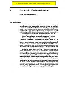
various states. For example, a road cell can be occupied by a vehicle or be empty. Local transition rules determine the dynamics of the system and even simple rules can lead to a highly dynamic system. The GLD infrastructure consists of roads and nodes. A road connects two nodes, and can have several lanes in each direction. The length of each road is expressed in cells. A node is either an intersection where traffic lights are operational or an edge node. There are two types of agents that occupy such an infrastructure: vehicles and traffic lights (or intersections). All agents act autonomously and are updated every timestep. Vehicles enter the network at edge nodes and each edge node has a certain probability of generating a vehicle at each timestep (spawn rate). Each generated vehicle is assigned one of the other edge nodes as a destination. The distribution of destinations for each edge node can be adjusted. There can be several types of vehicles, defined by their speed, length, and number of passengers. In this chapter, all vehicles have equal length and an equal number of passengers. The state of each vehicle is updated every timestep. It either moves the distance determined by its speed and the state around it (e.g. vehicles in front may limit how far it can travel) or remains in the same position (e.g. the next position is occupied or a traffic light prevents its lane from moving). When a vehicle crosses an intersection, its driving policy determines which lane it goes to next. Once a lane is selected, the vehicle cannot switch to a different lane. For each intersection, there are multiple light configurations that are safe. At each timestep, the intersection must choose from among these configurations, given the current state. Figure 1 shows an example GLD intersection. It has four roads, each consisting of four lanes (two in each direction). Vehicles occupy n cells of a lane, depending on their length. Traffic on a given lane can only travel in the directions allowed on that lane. This determines the possible safe light configurations. For example, the figure shows a lane where traffic is only allowed to travel straight or right. The behavior of each vehicle depends on how it selects a path to its destination node and how it adjusts its speed over time. In our experiments, the vehicles always select the shortest path to their destination node.

3 Multiagent Reinforcement Learning for Urban Traffic Control Several techniques for learning traffic controllers with model-free reinforcement learning methods like Sarsa [30] or Q-learning [1, 19] have previously been developed. However, they all suffer from the same problem: they do not scale to large networks since the size of the state space grows rapidly. Hence, they are either applied only to small networks or are used to train homogeneous controllers (by training on a single isolated intersection and copying the result to each intersection in the network). Even though there is little theoretical support, many authors (e.g. [2, 27, 4]) have found that often, in practice, a more tractable approach, in terms of sample com-


5

Fig. 1 An example GLD intersection.

plexity, is to use some variation of model-based reinforcement learning, in which the transition and reward functions are estimated from experience and afterwards or simultaneously used to find a policy via planning methods like dynamic programming [5]. An intuitive reason for this is that such an approach can typically make more effective use of each interaction with the environment than model-free reinforcement learning. This is because the succession of states and rewards given actions contains much useful information about the dynamics of the environment which is ignored when one just learns a value function as in model-free learning, whereas it is fully used when one learns to predict the environment when learning the model. In practice, a learned model can typically be sufficiently accurate relatively quickly, and thus provide useful guidance for approximating the value function relatively quickly, compared to model-free learning. In the case of our traffic system, a full transition function would have to map the location of every vehicle in the system at one timestep to the location of every vehicle at the next timestep. Doing so is clearly infeasible, but learning a model is nonetheless possible if a vehicle-based representation [33] is used. In this approach, the global state is decomposed into local states based on each individual vehicle. The transition function maps one vehicle’s location at a given timestep to its location at the next timestep. As a result, the number of states grows linearly in the number of cells and can scale to much larger networks. Furthermore, the transition function can generalize from experience gathered in different locations, rather than having to learn separate mappings for each location.

6


To represent the model, we need only keep track of the number of times each transition (s, a, s0 ) has occurred and each state-action pair (s, a) has been reached. The transition model can then be estimated via the maximum likelihood probability, as described below. Hence, each timestep produces new data which is used to update the model. Every time the model changes, the value function computed via dynamic programming must be updated too. However, rather than having to update each state, we can update only the states most likely to be affected by the new data, using an approach based on prioritized sweeping [2]. The remainder of this section describes the process of learning the model in more detail. Given a vehicle-based representation, the traffic control problem consists of the following components: • s ∈ S: the fully observable global state • i ∈ I: an intersection (traffic junction) controller • a ∈ A: an action, which consists of setting to green a subset of the traffic lights at the intersection; Ai ⊆ A is the subset of actions that are safe at intersection i • l ∈ L: a traffic lane; Li ⊆ L is the subset of incoming lanes for intersection i • p ∈ P: a position; Pl ⊆ P is the subset of positions for lane l The global transition model is P(s0 |s, a) and the global state s decomposes into a vector of local states, s = hs pli i, with one for each position in the network. The transition model can be estimated using maximum likelihoods by counting state transitions and corresponding actions. The update is given by: C(s pli , ai , s0pl )

P(s0pl |s pli , ai ) := i

ij

C(s pli , ai )

(1)

where C(·) is a function that counts the number of times the event (state transition) occurs. To estimate the value of local states (discussed below), we also need to estimate the probability that a certain action will be taken given the state (and the policy), which is done using the following update: P(ai |s pli ) :=

C(s pli , ai )

(2)

C(s pli )

It is important to note that this does not correspond to the action selection process itself (cf. Eq. 9) or learning of the controller (cf. Eq. 7), but rather an estimate of the expected action, which is necessary below in Equation 8. The global reward function decomposes as: r(s, s0 ) = ∑ ∑ ∑ r(s pli , s0pl ) i

and

li pli

½ r(s pli , s0pl ) = i

i

0 s pli 6= s0pl i −1 otherwise

(3)

(4)


7

Thus, if and only if a car stays in the same place the reward (cost) is −1. This means that values estimated by the value function learned using (multiagent) reinforcement learning will reflect total waiting time of cars, which must be minimized. Since the value function essentially represents the sum of the waiting times of individual cars at individual junctions, the action-value function decomposes as: Q(s, a) = ∑ Qi (si , ai )

(5)

i

where si is the local state around intersection i and ai is the local action (safe traffic light configuration) at this intersection, and Qi (si , ai ) = ∑ ∑ Q pli (s pli , ai ).

(6)

li pli

Given the current model, the optimal value function is estimated using dynamic programming, in this case value iteration [5, 26, 4], with a fixed number of iterations. We perform only one iteration per timestep [4, 2] and use ε -greedy exploration to ensure the estimated model obtains sufficiently diverse data. ε -greedy exploration usually takes the action that is currently estimated to be optimal given the current value function, but with probability ε takes a different random action. The vehiclebased update rule is then given by: Q pli (s pli , ai ) :=

∑

s0p ∈S0

P(s0pl |ai , s pli )[r(s pli , s0pl ) + γ V (s0pl )] i

i

i

(7)

li

where S0 are all possible states that can be reached from s pli given the current traffic situation and the vehicle’s properties (e.g. its speed). V (s pli ) estimates the expected waiting time at pli and is given by: V (s pli ) := ∑ P(ai |s pli )Q(s pli , ai ).

(8)

ai

We use a discount parameter γ = 0.9. In reinforcement learning and dynamic programming, the discount parameter discounts future rewards, and depending on the value (between 0 and 1) lets the agent pay more attention to short-term reward as opposed to long-term reward (see [26]). Note also that similar to prioritized sweeping [2], at each timestep only local states that are directly affected (because there are cars driving over their corresponding cells) are updated. At each time step, using the decomposition of the global state, the joint action (traffic light settings) currently estimated to be optimal (given the value function) is determined as follows: π ∗ (s) = arg max Q(s, a) (9) a

where arg maxa Q(s, a), which is the optimal global action vector a, in this model corresponds to the optimal local action for each intersection i, i.e. arg maxai Q(si , ai ), which can in turn be decomposed as

8


arg max Q(si , ai ) = arg max ∑ ∑ O pli Q pli (s pli , ai ) ai

ai

(10)

li pli

where O pli is a binary operator which indicates occupancy at pli : ½ 0 if pli not occupied O pli = 1 otherwise

(11)

4 Representing and handling traffic congestion The method described above has already been shown to outperform alternative, nonlearning traffic light controllers [33, 34, 35]. Nevertheless, there is still considerable room for improvement. In the basic method (called Traffic Controller-1 or TC-1 in the original papers [33, 34, 35], and for this reason we will stay with this naming convention), traffic light decisions are made based only on local state information around a single junction. Taking into account traffic situations at other junctions may improve overall performance, especially if these traffic situations are highly dynamic and may include both free flowing traffic and traffic jams (congestion). For example, there is no use in setting lights to green for cars that, further on in their route, will have to wait anyway because there traffic is congested completely. The two extensions described in this section extend the method described above based on these considerations. The basic idea in both new methods is to keep the principle of local optimization of traffic light junctions, in order to keep the methods computationally feasible. However, traffic light junctions will now take into account, as extra information, the amount of traffic at neighboring junctions, a “congestion factor”. This means that next to local state information, more distant, global (nonlocal) information is also used for traffic light optimization.

4.1 TC-SBC method The first extension proposed in this section takes into account traffic situations at other places in the traffic network by including congestion information in the state representation. The cost of including such congestion information is a larger state space and potentially slower learning. The value function Q pli (s pli , ai ) is extended to Q pli (s pli , c pli , ai ) where c pli ∈ {0, 1} is a single bit indicating the congestion level at the next lane for the vehicle currently at pli . If the congestion at the next lane exceeds a threshold then c pli = 1 and otherwise it is set to 0. This extension allows the agents to learn different state transition probabilities and value functions when the outbound lanes are congested. We call this method the “State Bit for Congestion” (TC-SBC) method. Specifically, first a real-valued congestion factor kdest p is computed for each car at pli : li


kdest p = li

wdest p

9

li

(12)

Ddest p

li

where wdest p is the number of cars on destination lane dest pli , and Ddest p is the li

li

number of available positions on that destination lane dest pli . The congestion bit c pli , which determines the table entry for the value function, is computed according to ( 1 if kdest p > θ li c pli = (13) 0 otherwise where θ is a parameter acting as a threshold. Like before, the transition model and value function are estimated online using maximum likelihood estimation and dynamic programming. But unlike before, now the system effectively learns different state transition probabilities and value functions when the neighboring roads are congested and when they are not congested (determined by the congestion bit). This makes sense, because the state transition probabilities and expected waiting times are likely to be widely different for these two cases. This allows the system to effectively learn different controllers for the cases of congestion and no congestion. An example of how this may lead to improved traffic flow is that a traffic light may learn that if (and only if) traffic at the next junction is congested, the expected waiting time for cars in that direction is almost identical when this traffic light is set to green compared to when it is set to red. Therefore, it will give precedence to cars going in another direction, where there is no congestion. At the same time, this will give the neighboring congested traffic light junction more time to resolve the congestion.

4.2 TC-GAC method A disadvantage of the TC-SBC method described above (cf. Section 4.1, Eq. 12 and 13) is that it increases the size of the state space. That is, in fact, the main reason for restricting the state expansion to only one bit indicating congestion for only the immediate neighbor. The second new method to deal with congestion investigated in this section does not expand the state space, but instead uses the congestion factor kdest p (described above) in a different way. li

Rather than quantizing the real-valued kdest p to obtain an additional state bit, li it is used in the computation of the estimated optimal traffic light configuration (cf. Eq. 10): arg max Q(si , ai ) = arg max ∑ ∑ O pli (1 − kdest p )Q pli (s pli , ai ) ai

ai

li pli

li

(14)

10


Thus, the congestion factor kdest p is subtracted from 1 such that the calculated li

value for an individual car occupying position pli given a particular traffic light configuration (representing its estimated waiting time given that it will see a red or a green light) will be taken fully into account when its next lane is empty (it is then multiplied by 1), or will not be taken into account at all if the next lane is fully congested (it is then multiplied by 0). We call this method the “Gain Adapted by Congestion” (TC-GAC) method, because it does not affect the value function estimation itself, but only the computation of the gain, in the decision theory sense, of setting traffic lights to green as opposed to red for cars that face or do not face congestion in their desitination lanes. The advantage of this method is that it does not increase the size of the state space, while making full use of real-valued congestion information. The disadvantage is that unlike TC-SBC, TC-GAC never learns anything permanent about congestion, and the method is even more specific to this particular application domain and even less generalizable to other domains—at least the principle of extending the state space to represent specific relevant situations that may require different control, as used by TC-SBC, can be generalized to other domains. Note that GAC can in fact be combined with SBC, because it is, in a sense, an orthogonal extension. We call the combination of the two the TC-SBC+GAC method.

4.3 Experimental Results 4.3.1 Test domains We tested our algorithms using the GLD simulator (section 2). We used the same traffic network, named Jillesville, as the one used in [34, 35] (see Figure 2), and compared our test results to the results of the basic MARL algorithm (TC-1, section 3). The original experiments [34, 35, 33] were all done with fixed spawning rates, i.e. fixed rates of cars entering the network at the edge nodes. We replicate some of those experiments, but also added experiments (using the same road network) with dynamic spawning rates. In these experiments, spawning rates change over time, simulating the more realistic situation of changes in the amount of traffic entering and leaving a city, due to rush hours etc. In all simulations we measure the Average Trip Waiting Time (ATWT), which corresponds to the amount of time spent waiting rather than driving. It is possible that traffic becomes completely jammed due to the large numbers of cars entering the road network. In that case we set ATWT to a very large value (50). We did preliminary experiments to find a good parameter setting of the congestion threshold parameter θ for the TC-SBC method. θ = 0.8 gave the best results in all cases, also for the TC-SBC+GAC method, so we are using that value in the experiments described below. It is worth noting that even though TC-SBC adds another parameter, apparently one parameter value works well for different variations


11

Fig. 2 The Jillesville infrastructure.

of the problem and the algorithm, and no parameter tuning is required for every specific case.

4.3.2 Experiment 1: Fixed spawning rate As described above, we performed simulations to compare our new congestionbased RL controllers (TC-SBC, TC-GAC, TC-SBC+GAC, section 3) to the original RL controller (TC-1, section 2.3) in one of the original test problems. This test problem corresponds to Wiering’s experiment 1 [34, 35] and uses the road network depicted in Figure 2. The spawning rate is fixed and set to 0.4. Each run corresponds to 50,000 cycles. For each experimental condition (controller type) 5 runs were done and the results were averaged. We found that 5 runs sufficed to obtain sufficiently clear and distinct results for the different experimental conditions, but no statistical significance was determined. Figure 3 shows the overall results of the experiment. The Average Trip Waiting Time (ATWT) is depicted over time. Each curve represents the average of 5 runs. The most important result is that all of our new methods lead, in the long run, to

12

Bram Bakker and Shimon Whiteson and Leon J.H.M. Kester and Frans C.A. Groen 30

25

ATWT(cycles)

20

15

10

5

0

0

0.5

1

1.5

2

2.5

3

3.5

4

cycles TC−SBC

TC−SBC+GAC

4.5

5 4

x 10 TC−1

TC−GAC

Fig. 3 Performance of our congestion-based controllers versus TC-1, in the fixed spawning rate simulation (experiment 1).

better performance, i.e. lower ATWT, than the original method TC-1. The best performance in this test problem is obtained by TC-SBC+GAC, the method that combines both ways of using congestion information. Interestingly, in the initial stages of learning this method has, for a while, the worst average performance, but then it apparently learns a very good value function and corresponding policy, and reduces ATWT to a very low level. This relatively late learning of the best policy may be caused by the learning system first learning a basic policy and later fine-tuning this based on the experienced effects of the GAC component. Figure 4 shows a snapshot of part of the traffic network in the traffic simulator during one run, where the controller was TC-SBC+GAC. A darker traffic junction indicates a more congested traffic situation around that junction. The lower right junction is fairly congested, which results in the traffic lights leading to that junction to be set to red more often and for longer periods of time.

4.3.3 Experiment 2: Dynamic spawning rate, rush hours Experiment 2 uses the same traffic network (Figure 2) as experiment 1, but uses dynamic spawning rates rather than fixed ones. These simulations similarly last for 50,000 cycles and start with spawning rate 0.4. Every run is divided into five blocks of 10,000 cycles, within each of which at cycle 5,000 “rush hour” starts and the spawning rate is set to 0.7. At cycle 5,500 the spawning rate is set to 0.2, and at cycle 8,000 the spawning rate is set back to 0.4 again. The idea is that especially


13

Fig. 4 Snapshot of part of the traffic network in the traffic simulator. Darker nodes indicate more congested traffic.

in these dynamic situations traffic flow may benefit from our new methods, which dynamically take into account congestion. Figure 5 shows the results. As in experiment 1, all of our new methods outperform the original, TC-1 method. As expected, the difference is actually more pronounced (note the scale of the graph): TC-SBC, TC-GAC, and TC-SBC+GAC are much better in dealing with the changes in traffic flow due to rush hours. Rush hours do lead to longer waiting times temporarily (the upward “bumps” in the graph). However, unlike the original, TC-1 method, our methods avoid getting complete traffic jams, and after rush hours they manage to reduce the Average Trip Waiting Time. The best method in this experiment is TC-GAC. It is not entirely clear why TC-GAC outperforms the version with SBC, but it may have to do with the fact that the increased state space associated with SBC makes it difficult to obtain a sufficient amount of experience for each state in this experiment where there is much variation in traffic flow.

5 Partial observability In the work described so far we assumed that the traffic light controllers have access, in principle, to all traffic state information, even if the system is designed such that agents make decisions based only on local state information. In other words, we made the assumption of complete observability of the MDP (see Figure 6). In the real world it is often not realistic to assume that all state information can be gathered or that the gathered information is perfectly accurate. Thus decisions typically have

14

Bram Bakker and Shimon Whiteson and Leon J.H.M. Kester and Frans C.A. Groen 45

40

35

ATWT(cycles)

30

25

20

15

10

5

0

0

0.5

1

1.5

2

2.5

3

3.5

4

cycles TC−SBC

TC−SBC+GAC

4.5

5 4

x 10 TC−1

TC−GAC

Fig. 5 Performance of our congestion-based controllers versus TC-1, in the dynamic spawning rate simulation (experiment 2, “rush hours”).

to be made based on incomplete or erroneous information. This implies dealing with partial observability. In order to obtain full observability in a real world implementation of the traffic control system, a similar grid like state discretization as is the case in our GLD traffic simulation would have to be made on roads, with a car sensor (e.g. an induction loop sensor) for each discrete state. On a real road the amount of sensors needed to realize this is immense; moreover, road users do not move from one discrete state to another, but move continuously. Approximating the state space by using fewer sensors converts the problem from completely to partially observable. The controller no longer has direct access to all state information. The quality of the sensors, i.e. the possibility of faulty sensor readings, also plays a role in partial observability. In this section we study partial observability within our multiagent reinforcement learning for traffic light control framework. To model partial observability in the —up to now fully observable— traffic simulator an observation layer is added. This allows algorithms to get their state information through this observation layer instead. Multiagent systems with partial observability constitute a domain not heavily explored, but an important one to make a link to real world application and realistic traffic light control. Most of the already developed algorithms for partial observability focus on single agent problems. Another problem is that many are too computationally intensive to solve tasks more complex than toy problems. Adding the multiagent aspect increases the complexity considerably, because the size of the joint action space is exponential in the number of agents. Instead of having to compute a best action based on one agent, the combined (joint) best action needs to


15

be chosen from all the combinations of best actions of single agents. In the traffic light controller work described in this chapter so far, this problem is addressed by decomposing into local actions, each of which is optimized individually, and this same approach is used here. For the single agent case, to diminish the computational complexity several heuristic approximations for dealing with partial observability have been proposed. Primary examples of these heuristic approximations are the Most Likely State (MLS) approach and Q-MDP [6]. Our approach will be be based on these approximations, and can be viewed as a multiagent extension.

5.1 POMDPs Partially Observable Markov Decision Processes, or POMDPs for short, are Markov Decision Processes (the basis for all work described above) in which the state of the environment, which itself has the Markov property, is only partially observable, such that the resulting observations do not have the Markov property (see [6, 13, 20] for introductions to POMDPs). For clarity we will, in this section, refer to MDPs, including the traffic light systems described above which are non-standard variations of MDPs, as Completely Observable MDPs (or COMDPs). A POMDP is denoted by the tuple Ξ = (S, A, Z, R, P, M), where S, A, P, and R are the same as in COMDPs. Z is the set of observations. After a state transition one of these observations o is perceived by the agent(s). M is the observation function, M : S × A → Π (Z), mapping states-action pairs to a probability distribution over the observations the agent will see after doing that action from that state. As can be seen, the observation function is dependent on the state the agents is in and the action it executes. Importantly, in contrast to (standard) COMDPs, the agent no longer directly perceives the state (see Figure 6), but instead perceives an observation which may give ambiguous information regarding the underlying state (i.e. there is hidden state), and must do state estimation to obtain its best estimate of the current state (see Figure 7).

5.2 Belief states A POMDP agent’s best estimate of the current state is obtained when it remembers the entire history of the process [32][6]. However it is possible to “compress” the entire history intto a summary state, a belief state, which is a sufficient statistic for the history. The belief state is a probability distribution over the state space: B = Π (S), denoting for each state the probability that the agent is in that state, given the history of observations and actions. The policy can then be based on the entire history, π : B → A. Unlike the complete history however, the belief state B is of fixed size, while the history grows with each time step. In contrast to the POMDP

16


Fig. 6 The generic model of an agent in a (completely observable) MDP. At each time step, the agent performs actions in its environment, and in response receives information about the new state that it is in as well as an immediate reward (or cost).

Fig. 7 The POMDP model: since states are no longer directly observable, they will have to be estimated from the sequence of observations following actions. This is done by the state estimation module, which outputs a belief state b to be used by the policy.

observations, the POMDP belief state has the Markov property, subsequent belief states only depend on the current belief state and no additional amount of history about the observations and actions can improve the information contained in the belief state. The notation for the belief state probability will be b(s), the probabilities that the agent is in each (global) state s ∈ S. The next belief state depends only on the previous belief state and the current action and observation, and is computed using Bayes’ rule [6].


17

Fig. 8 Sensors on fully and partially observable roads.

5.3 Partial observability in the traffic system Figure 8 shows a single traffic lane in our simulator, both for the completely (fully) observable case, as was used in the work described in the previous sections, and for the partially observable case. In the latter case, there are car sensors e which provide noisy information e(s) about the occupation of the network position where they are placed, and they are placed only at the very beginning and very end of each lane, which means that for the intermediate positions nontrivial state estimation must be done. In order to get a good belief state of a drive lane bd such as depicted in Figure 8, it is necessary first of all to create a belief state for individual road users, b f . To create b f , sensor information can be used in combination with assumptions that can be made for a road user. Actions u f are the actions of the road user f . Suppose the sensors inform the system of road user being on the beginning of the road on time step t = 0, then given that cars may move at different speeds, the car may move 1, 2, or 3 steps forward. This means that the road user is on either position 1, position 2, or position 3 of the road on time step t = 1. By the same logic, the whole b f of all cars can be computed for all time steps, using the Bayes update rule: b f (st ) = p(zt |st ) ∑ p(st |u f ,t , st−1 )p(st−1 |zt−1 , ut−1 )

(15)

st−1

Since there are many cars, calculating only belief states of individual road users and assuming that those individual road users are not dependent on each other’s position is not correct. Therefore, to calculate the belief state for the whole driving lane, bd , all the b f for that driving lane must be combined, taking into account their respective positions. bdpl denotes the individual probability, according to the comi

plete belief state bd , of a car being at position p of lane l at intersection (junction) i. Three additional principles guide the algorithm that computes the belief state for the combination of all cars in the network. Firstly, road users that arrive on a lane at a later t cannot pass road users that arrived at an earlier t. Secondly, road users

18


cannot be on top of each other. Thirdly, road users always move forward as far as they can, leaving room behind them when they can, such that road users arriving at a later time step have a spot on the road. The exact algorithm incorporating this can be found in [24]. Figure 9 shows an example belief state for the whole driving lane, bd , for one lane in a traffic network.

Fig. 9 The probability distribution of bd is shown for a drive lane of the Jillesville infrastructure.

5.4 Multiagent Most-Likely-State and Q-MDP This section describes multiagent variations to two well-known heuristic approximations for POMDPs, the Most Likely State (MLS) approach and Q-MDP [6]. Both are based on estimating the value function as if the system is completely observable, which is not optimal but works well in many cases, and then combining this value function with the belief state. The MLS approach simply assumes that the most likely state in the belief state is the actual state, and chooses actions accordingly. Two types of Most Likely State implementations are investigated here. In the first, we use the individual road user beliefstate (for all road users):


sMLS = arg max b f (s) f

19

(16)

s

and, as before, a binary operator which indicates occupancy of a position in the road network by a car is defined: ½ 1 if pli corresponds to an s pli ∈ sMLS f = OMLS (17) pli 0 otherwise. Thus, the difference with occupancy as defined in the standard model in Eq. 11 is that here occupancy is assumed if this is indicated by the most likely state estimation. Action selection is done as follows: arg max Q(si , ai ) = arg max ∑ ∑ OMLS Q pli (s pli , ai ) pl ai

ai

i

li pli

(18)

The second type of MLS implementation uses bd , the belief state defined for a drive lane, which is more sophisticated and takes into account mutual constraints between cars. With this belief state the state can be seen as the possible queues of road users for that drive lane. The MLS approximation for this queue is called the Most Likely Queue, or MLQ. The most like queue is: sMLQ = arg max bd (s) d s

and

( = OMLQ pl i

1 if pli corresponds to an s pli ∈ sdMLQ 0 otherwise

(19)

(20)

and action selection is done as follows: Q pli (s pli , ai ). arg max Q(si , ai ) = arg max ∑ ∑ OMLQ pl ai

ai

li pli

i

(21)

Instead of selecting the most like state (or queue) from the belief state, the idea of Q-MDP is to use the entire belief state: the state-action value function is weighed by the probabilities defined by the belief state, allowing all possible occupied states to have a “vote” in the action selection process and giving greater weight to more likely states. Thus, action selection becomes: arg max Q(si , ai ) = arg max ∑ ∑ bdpl Q pli (s pli , ai ). ai

ai

li pli

i

(22)

In single agent POMDPs, Q-MDP usually leads to better results than MLS [6]. To provide a baseline method for comparison, a simple method was implemented as well: the All In Front, or AIF, method assumes that all the road users that are detected by the first sensor are immediately at the end of the lane, in front of the traffic light. The road users are not placed on top of each other. Then the decision for the configuration of the traffic lights is based on this simplistic assumption. Further-

20


more, we compare with the standard TC-1 RL controller, referred to as COMDP here, that has complete observability of the state.

5.5 Learning the Model MLS/MLQ and Q-MDP provide approximate solutions for the partially observable traffic light control system, given that the state transition model and value function can still be learned as usual. However, in the partially observable case the model cannot be learned by counting state transitions, because the states cannot directly be accessed. Instead, all the transitions between the belief state probabilities of the current state and the probabilities of the next belief states should be counted to be able to learn the model. Recall, however, that belief states have a continuous state space even if the original state space is discrete, so there will in effect be an infinite number of possible state transitions to count at each time step. This is not possible. An approximation is therefore needed. The following approximation is used: learning the model without using the full belief state space, but just using the belief state point that has the highest probability, as in MLS/MLQ. Using the combined road user beliefstate bd , the most likely states in this beliefstate are sMLQ . The local state (being occupied or not) at position p of lane l at intersection (junction) i, according to the most likely queue estimate, is denoted by sMLQ . Assuming these most likely states are the correct states, the pli system can again estimate the state transition model by counting the transitions of road users as if the state were fully observable (cf. eq. 1: P(s0pl |s pli , ai ) := i

C(sMLQ , ai , sMLQ pli pli j ) C(sMLQ , ai ) pli

(23)

and likewise for the other update rules (cf. section 3). Although this approximation is not optimal, it provides a way to sample the model and the intuition is that with many samples it provides a fair approximation.

5.6 Test Domains The new algorithms were tested on two different traffic networks, namely the Jillesville traffic network used before (see Figure 2), and a newly designed simple network named LongestRoad. Since Jillesville was used in previous work it is interesting to use it for partial observability as well, and to see if it can still be controlled well under partial observability. Jillesville is a traffic network with 16 junctions, 12 edge nodes or spawn nodes and 36 roads with 4 drive lanes each.


21

Fig. 10 The LongestRoad infrastructure.

LongestRoad (Figure 10) is, in most respects, a much simpler traffic network than Jillesville because it only has 1 junction, 4 edge nodes and 4 roads with 4 drive lanes each. The biggest challenge, however, in this set-up is that the drive lanes themselves are much longer than in Jillesville, making the probabilities of being wrong with the belief states a lot higher, given sensors only at the beginnings and ends of lanes. This was used to test the robustness of the POMDP algorithms. In the experiments described above (Section 4.3) the main performance measure was average traffic waiting time (ATWT). However, in the case of partial observability we found that many suboptimal controllers lead to complete congestion with no cars moving any more, in which case ATWT is not the most informative measure. Instead, here we use a measure called Total Arrived Road Users (TAR) which, as the name implies, is the number of total road users that actually reached their goal node. TAR measures effectively how many road users actually arrive at their goal and don’t just stand still forever. Furthermore, we specifically measure TAR as a function of the spawning rate, i.e. the rate at which new cars enter the network at edge nodes. This allows us to gauge the level of traffic load that the system can handle correctly, and observe when it breaks down and leads to complete or almost complete catastrophic congestion.

22


5.7 Experimental results: COMDP vs. POMDP algorithms Figure 11 shows the results, TAR as a function of spawning rate, for the different algorithms described above, when tested on the partially observable Jillesville traffic infrastructure. A straight monotically increasingly line indicates that all additional road users injected at higher spawning rates arrive at their destinations (because TAR scales linearly with the spawning rate, unless there are congestions). Here we do not yet have model learning under partial observability; the model is learned under full observability, and the focus in on how the controllers function under partial obsrvability. The results in Figure 11 show that Q-MDP performs very well, and is comparable to COMDP, with MLQ slightly behind the two top algorithms. AIF and MLS perform much worse; this is not very surprising as they make assumptions which are overly simplistic. The highest throughput is thus reached by Q-MDP since that algorithm has the most Total Arrived Road Users. This test also shows that the robustness of Q-MDP is better than the alternative POMDP methods since the maximum spawn rates for Q-MDP before the simulation gets into a “deadlock” situation (the sudden drop in the curves when spawn rates are pushed beyond a certain level) are higher. Generally the algorithms MLQ, Q-MDP, and COMDP perform at almost an equal level. 4

Jillesville

x 10 16

14

12

TAR

10

8

6

4

2

0 0.27

AIF COMDP MLQ MLS QMDP 0.31

0.35

0.39 spawnrate

0.43

0.47

0.51

Fig. 11 Results on the partially observable Jillesville traffic infrastructure, comparing POMDP with COMDP algorithms.

With the LongestRoad network, in which individual roads are substantially longer, a slightly different result can be observed (see Figure 12). In the Jillesville

Traffic Light Control by Multiagent Reinforcement Learning Systems 4

23

LongestRoad

x 10 7

6

TAR

5

4

3

2

1

0 0.24

AIF COMDP MLQ MLS QMDP 0.28

0.32 spawnrate

0.36

0.4

Fig. 12 Results on the partially observable LongestRoad traffic infrastructure, comparing POMDP with COMDP algorithms.

traffic network, MLS was underperforming, compared to the other methods. On the LongestRoad network on the other hand the performance is not bad. COMDP appears to perform slightly worse than the POMDP methods (except for AIF). In theory COMDP should be the upper bound, since its state space is directly accessible and the RL approach should then perform best. One possibility is that the COMDP algorithm has some difficulties converging on this infrastructure compared to other infrastructures because of the greater lengths of the roads. Longer roads provide more states and since a road user will generally not come across all states when it passes through (with higher speeds many cells are skipped), many road users are needed in order to get good model and value function approximations. The POMDP algorithms’ state estimation mechanism is somewhat crude, but perhaps this effectively leads to fewer states being considered and less sensitivity to inaccuracies of value estimations for some states. In any case, the performance of the most advanced POMDP and COMDP methods is comparable, and only the baseline AIF method and the simple MLS method perform much worse.

24


5.8 Experimental results: Learning the model under partial observability The experiment described above showed good results of making decisions under partial observability. Next we test the effectiveness of learning the model under partial observability. The methods doing that do so using the MLQ state (see above) and are indicated by MLQLearnt suffixes. We again compare with COMDP, and with the POMDP methods with complete observability model learning. We do not include AIF in this comparison, as it was already shown to be inferior above. The results on Jillesville are shown in Figure 13. It can be seen that the MLQLearnt methods works very well. MLQ-MLQLearnt (MLQ action selection and model learning based on MLQ) does not perform as well as Q-MDP-MLQLearnt (Q-MDP action selection and model learning based on MLQ), but still has a good performance on Jillesville. It can be concluded that in this domain, when there is partial observability, both action selection and model learning can be done effectively, given that proper approximation technques are used. We can derive the same conclusion from a similar experiment with the LongestRoad traffic network (see Figure 14). Again learning the model under partial observability based on the MLQ state does not negatively affect behavior. 4

Jillesville

x 10 16

14

12

TAR

10

8

6

4

2

0 0.27

COMDP MLQ MLQ−MLQLearnt QMDP QMDP−MLQLearnt 0.31

0.35

0.39 spawnrate

0.43

0.47

0.51

Fig. 13 Results on the partially observable Jillesville traffic infrastructure, comparing POMDP algorithms which learn the model under partial observability (MLQLearnt) with POMDP algorithms which do not have this additional difficulty.

Traffic Light Control by Multiagent Reinforcement Learning Systems 4

25

LongestRoad

x 10 7

6

TAR

5

4

3

2

1

0 0.24

COMDP MLQ MLQ−MLQLearnt QMDP QMDP−MLQLearnt 0.28

0.32 spawnrate

0.36

0.4

Fig. 14 Results on the partially observable LongestRoad traffic infrastructure, comparing POMDP algorithms which learn the model under partial observability (MLQLearnt) with POMDP algorithms which do not have this additional difficulty.

6 Multiagent coordination of traffic light controllers In the third and final extension to the basic multiagent reinforcement learning approach to traffic light control, we return to the situation of complete observability of the state (as opposed to partial observability considered in the previous section), but focus on the issue of multiagent coordination. The primary limitation of the approaches described above is that the individual agents (controllers for individual traffic junctions) do not coordinate their behavior. Consequently, agents may select individual actions that are locally optimal but that together result in global inefficiencies. Coordinating actions, here and in general in multiagent systems, can be difficult since the size of the joint action space is exponential in the number of agents. However, in many cases, the best action for a given agent may depend on only a small subset of the other agents. If so, the global reward function can be decomposed into local functions involving only subsets of agents. The optimal joint action can then be estimated by finding the joint action that maximizes the sum of the local rewards. A coordination graph [10], which can be used to describe the dependencies between agents, is an undirected graph G = (V, E) in which each node i ∈ V represents an agent and each edge e(i, j) ∈ E between agents i and j indicates a dependency between them. The global coordination problem is then decomposed into a set of local coordination problems, each involving a subset of the agents. Since any arbitrary graph can be converted to one with only pairwise dependencies [36], the global

26


action-value function can be decomposed into pairwise value functions given by: Q(s, a) =

∑

Qi j (s, ai , a j )

(24)

i, j∈E

where ai and a j are the corresponding actions of agents i and j, respectively. Using such a decomposition, the variable elimination [10] algorithm can compute the optimal joint action by iteratively eliminating agents and creating new conditional functions that compute the maximal value the agent can achieve given the actions of the other agents on which it depends. Although this algorithm always finds the optimal joint action, it is computationally expensive, as the execution time is exponential in the induced width of the graph [31]. Furthermore, the actions are known only when the entire computation completes, which can be a problem for systems that must perform under time constraints. In such cases, it is desirable to have an anytime algorithm that improves its solution gradually. One such algorithm is max-plus [16, 15], which approximates the optimal joint action by iteratively sending locally optimized messages between connected nodes in the graph. While in state s, a message from agent i to neighboring agent j describes a local reward function for agent j and is defined by:

µi j (a j ) = max{Qi j (s, ai , a j ) + ai

∑

µki (ai )} + ci j

(25)

k∈Γ (i)\ j

where Γ (i)\ j denotes all neighbors of i except for j and ci j is either zero or can be used to normalize the messages. The message approximates the maximum value agent i can achieve for each action of agent j based on the function defined between them and incoming messages to agent i from other connected agents (except j). Once the algorithm converges or time runs out, each agent i can select the action a∗i = arg max ai

∑

µ ji (ai )

(26)

j∈Γ (i)

Max-plus has been proven to converge to the optimal action in finite iterations, but only for tree-structured graphs, not those with cycles. Nevertheless, the algorithm has been successfully applied to such graphs [8, 15, 36].

6.1 Max-Plus for Urban Traffic Control Max-plus enables agents to coordinate their actions and learn cooperatively. Doing so can increase robustness, as the system can become unstable and inconsistent when agents do not coordinate. By exploiting coordination graphs, max-plus minimizes the expense of computing joint actions and allows them to be approximated within time constraints. In this chapter, we combine max-plus with the model-based approach to traffic control described above. We use the vehicle-based representation defined in Sec-


27

tion 3 but add dependence relationships between certain agents. If i, j ∈ J are two intersections connected by a road, then they become neighbors in the coordination graph, i.e. i ∈ Γ ( j) and j ∈ Γ (i). The local value functions are: Qi (si , ai , a j ) = ∑ ∑ Q pli (s pli , ai , a j )

(27)

li pli

Using the above, we can define the pairwise value functions used by max-plus: Qi j (s, ai , a j ) = ∑ O pli Q pli (s pli , ai , a j ) + ∑ O pl j Q pl j (s pl j , a j , ai ) pli

(28)

pl j

where O pli is the binary operator which indicates occupancy at pli (eq. 11). These local functions are plugged directly into Equation 25 to implement maxplus. Note that the functions are symmetric such that Qi j (s, ai , a j ) = Q ji (s, a j , ai ). Thus, using Equation 28, the joint action can be estimated directly by the max-plus algorithm. Like before, we use one iteration of dynamic programming per timestep and ε -greedy exploration. We also limit max-plus to 3 iterations per timestep. Note that there are two levels of value propagation among agents. On the lower level, the vehicle-based representation enables estimated values to be propagated between neighboring agents and eventually through the entire network, as before. On the higher level, agents use max-plus when computing joint actions to inform their neighbors of the best value they can achieve, given the current state and the values received from other agents. Using this approach, agents can learn cooperative behavior, since they share value functions with their neighbors. Furthermore, they can do so efficiently, since the number of value functions is linear in the induced width of the graph. Stronger dependence relationships could also be modeled, i.e. between intersections not directly connected by a road, but we make the simplifying assumption that it is sufficient to model the dependencies between immediate neighbors in the traffic network.

6.2 Experimental Results In this section, we compare the novel approach described in Section 6.1 to the TC1 (Traffic Controller 1) described in section 3 and the TC-SBC (Traffic Controller with State Bit for Congestion) extension described in section 4 (we do not compare to TC-GAC as that is not really a learning method and is very specific to the particular application domain and not easily generalizable). We focus our experiments on comparisons between the coordination graph/max-plus method, TC-1, and TC-SBC in saturated traffic conditions (i.e. a lot of traffic, close to congestion), as these are conditions in which differences between traffic light controllers become apparent and coordination may be important.

28


These experiments are designed to test the hypothesis that, under highly saturated conditions, coordination is beneficial when the amount of local traffic is small. Local traffic consists of vehicles that cross a single intersection and then exit the network, thereby interacting with just one learning agent (traffic junction controller). If this hypothesis is correct, coordinated learning with max-plus should substantially outperform TC-1 and TC-SBC in particular when most vehicles pass through multiple intersections. In particular, we consider three different scenarios. In the baseline scenario, the traffic network includes routes, i.e. paths from one edge node to another, that cross only a single intersection. Since each vehicle’s destination is chosen from a uniform distribution, there is a substantial amount of local traffic. In the nonuniform destinations scenario, the same network is used but destinations are selected to ensure that each vehicle crosses two or more intersections, thereby eliminating local traffic. To ensure that any performance differences we observe are due to the absence of local traffic and not just to a lack of uniform destinations, we also consider the long routes scenario. In this case, destinations are selected uniformly but the network is altered such that all routes contain at least two intersections, again eliminating local traffic. While a small amount of local traffic will occur in real-world scenarios, the vast majority is likely to be non-local. Thus, the baseline scenario is used, not for its realism, but to help isolate the effect of local traffic on each method’s performance. The nonuniform destinations and long routes scenarios are more challenging and realistic, as they require the methods to cope with an abundance of non-local traffic. We present initial proof-of-concept results in small networks and then study the same three scenarios in larger networks to show that the max-plus approach scales well and that the qualitative differences between the methods are the same in more realistic scenarios. For each case, we consider again the metric of average trip waiting time (ATWT): the total waiting time of all vehicles that have reached their destination divided by the number of such vehicles. All results are averaged over 10 independent runs.

6.2.1 Small Networks Figure 15 shows the small network used for the baseline and nonuniform destinations scenarios. Each intersection allows traffic to cross from only one direction at a time. All lanes have equal length and all edge nodes have equal spawning rates (vehicles are generated with probability 0.2 per timestep). The left side of Figure 16 shows results from the baseline scenario, which have uniform destinations. As a result, much of the traffic is local and hence there is no significant performance difference between TC-1 and max-plus. TC-SBC performs worse than the other methods, which is likely due to slower learning as a result of a larger state space, and a lack of serious congestion, which is the situation that TC-SBC was designed for. The right side of Figure 16 shows results from the nonuniform destinations scenario. In this case, all traffic from intersections 1 and 3 is directed to intersection 2. Traffic from the top edge node of intersection 2 is directed to intersection 1 and


29

Fig. 15 The small network used in the baseline and nonuniform destinations scenarios.

traffic from the left edge node is directed to intersection 3. Consequently, there is no local traffic. This results in a dramatic performance difference between max-plus and the other two methods. This result is not surprising since the lack of uniform destinations creates a clear incentive for the intersections to coordinate their actions. For example, the lane from intersection 1 to 2 is likely to become saturated, as all traffic from edge nodes connected to intersection 1 must travel through it. When such saturation occurs, it is important for the two intersections to coordinate, since allowing incoming traffic to cross intersection 1 is pointless unless intersection 2 allows that same traffic to cross in a “green wave”. To ensure that the performance difference between the baseline and nonuniform destinations scenarios is due to the removal of local traffic and not some other effect of nonuniform destinations, we also consider the long routes scenario. Destinations are kept uniform, but the network structure is altered such that all routes involve at least two intersections. Figure 17 shows the new network, which has a fourth intersection that makes local traffic impossible. Figure 18 shows the results from this scenario. As before, max-plus substantially outperforms the other two methods, suggesting its advantage is due to the absence of local traffic rather than other factors. TC-1 achieves a lower ATWT than TC-SBC but actually performs much worse. In fact, TC-1’s joint actions are so poor that the outbound lanes of some edge nodes become full. As a result, the ATWT is not updated, leading to an artificially low score. At the end of each run, TC-1 had a much higher number cars waiting to enter the network than TC-SBC, and max-plus had none.

30


300 TC−1 TC−SBC max−plus

250

ATWT

200

150

100

50

0

0

1

2

3

4

timestep

5 4

x 10


400 350

ATWT

300 250 200 150 100 50 0

0

1

2

3 timestep

4

5 4

x 10

Fig. 16 Average ATWT per timestep for each method in the small network for the baseline (top) and nonuniform destinations (bottom) scenarios.

6.2.2 Large Networks We also consider the same three scenarios in larger networks, similar to the Jillesville network we worked with before (see Figure 2), to show that the max-plus approach scales well and that the qualitative differences between the methods are the same in more realistic scenarios. Figure 19 shows the network used for the baseline and nonuniform destinations scenarios. It includes 15 agents and roads with four lanes.


31

Fig. 17 The small network used in the long routes scenario.


450 400 350

ATWT

300 250 200 150 100 50 0

0

1

2

3 timestep

4

5 4

x 10

Fig. 18 Average ATWT per timestep in the small network for the long routes scenario.

The left side of Figure 20 shows results from the baseline scenario, which has uniform destinations. As with the smaller network, max-plus and TC-1 perform very similarly in this scenario, though max-plus’s coordination results in slightly slower learning. However, TC-SBC no longer performs worse than the other two methods, probably because the network is now large enough to incur substantial congestion. TC-SBC, thanks to its congestion bit, can cope with this occurrence better than TC1. The right side of Figure 20 shows results from the nonuniform destinations scenario. In this case, traffic from the top edge nodes travel only to the bottom edge nodes and vice versa. Similarly, traffic from the left edge nodes travel only to right edge nodes and vice versa. As a result, all local traffic is eliminated and max-plus performs much better than TC-1 and TC-SBC. TC-SBC performs substantially better than TC-1, as the value of its congestion bit is even greater in this scenario.

32


Fig. 19 The large network, similar to Jillesville, used in the baseline and nonuniform destinations scenarios.

To implement the long routes scenario, we remove one edge node from the two intersections that have two edge nodes (the top and bottom right nodes in Figure 19). Traffic destinations are uniformly distributed but the new network structure ensures that no local traffic occurs. The results of the long routes scenario are shown in Figure 21. As before, max-plus substantially outperforms the other two methods, confirming that its advantage is due to the absence of local traffic rather than other factors.

6.3 Discussion of max-plus results The experiments presented above demonstrate a strong correlation between the amount of local traffic and the value of coordinated learning. The max-plus method consistently outperforms both non-coordinated methods in each scenario where local traffic has been eliminated. Hence, these results help explain under what circum-


33


ATWT

10

5

0

0

1

2

3

4

timestep

5 4

x 10


350 300

ATWT

250 200 150 100 50 0

0

1

2

3 timestep

4

5 4

x 10

Fig. 20 Average ATWT per timestep for each method in the large network for the baseline (top) and nonuniform destinations (bottom) scenarios.

stances coordinated methods can be expected to perform better. More specifically, they confirm the hypothesis that, under highly saturated conditions, coordination is beneficial when the amount of local traffic is small. Even when there is substantial local traffic, the max-plus method achieves the same performance as the alternatives, though it learns more slowly. Hence, this method appears to be substantially more robust, as it can perform well in a much broader range of scenarios.

34


250 TC−1 TC−SBC max−plus 200

ATWT

150

100

50

0

0

1

2

3 timestep

4

5 4

x 10

Fig. 21 Average ATWT per timestep for each method in the long routes scenario.

By testing both small and large networks, the results also demonstrate that maxplus is practical in realistic settings. While max-plus has succeeded in small applications before [15], this chapter presents its first application to a large-scale problem. In fact, in the scenarios without local traffic, the performance gap between maxplus and the other methods was consistently larger in the big networks than the small ones. In other words, as the number of agents in the system grows, the need for coordination increases. This property makes the max-plus approach particularly attractive for solving large problems with complex networks and numerous agents. Finally, these results also provide additional confirmation that max-plus can perform well on cyclic graphs. The algorithm has been shown to converge only for tree-structured graphs, though empirical evidence suggests it also excels on small cyclic graphs [15]. The results presented in this chapter show that this performance also occurs in larger graphs, even if they are not tree-structured.

7 Conclusions This chapter presented several methods for learning efficient urban traffic controllers by multiagent reinforcement learning. First, the general multiagent reinforcement learning framework used to control traffic lights in this chapter was described. Next, three extensions were described which improve upon the basic framework in various ways: agents (traffic junctions) taking into account congestion information from neighboring agents; handling partial observability of traffic states; and coordinating the behavior of multiple agents by coordination graphs.


35

In the first extension, letting traffic lights take into account the level of traffic congestion at neighboring traffic lights had a beneficial influence on the performance of the algorithms. The algorithms using this new approach always performed better than the original method if there is traffic congestion, in particular when traffic conditions are highly dynamic such as is the case when there are both quiet times and rush hours. In the second extension, partial observability of the traffic state was successfully overcome by estimating belief states and combining this with multiagent variants of approximate POMDP solution methods. These variants are the Most Likely State (MLS) approach and Q-MDP, previously only used in the single case. It was shown that the state transition model and value function could also be estimated (learned) effectively under partial observability. The third extension extends the MARL approach to traffic control to include explicit coordination between neighboring traffic lights. Coordination is achieved using the max-plus algorithm, which estimates the optimal joint action by sending locally optimized messages among connected agents. This work presents the first application of max-plus to a large-scale problem and thus verifies its efficacy in realistic settings. Empirical results on both large and small traffic networks demonstrate that max-plus performs well on cyclic graphs, though it has been proven to converge only for tree-structured graphs. Furthermore, the results provide a new understanding of the properties a traffic network must have for such coordination to be beneficial and show that max-plus outperforms previous methods on networks that possess those properties. Acknowledgements The research reported here is part of the Interactive Collaborative Information Systems (ICIS) project, supported by the Dutch Ministry of Economic Affairs, grant nr: BSIK03024. The authors wish to thank Nikos Vlassis, Merlijn Steingröver, Roelant Schouten, Emil Nijhuis, and Lior Kuyer for their contributions to this chapter, and Marco Wiering for his feedback on several parts of the research described here.

References 1. B. Abdulhai, et al. Reinforcement Learning for True Adaptive Traffic Signal Control. In ASCE Journal of Transportation Engineering, 129(3): pg. 278-285, 2003. 2. A.W. Moore and C.G. Atkenson, Prioritized Sweeping: Reinforcement Learning with less data and less time, in Machine Learning, 13:103-130, 1993. 3. B. Bakker, M. Steingrover, R. Schouten, E. Nijhuis and L. Kester, Cooperative multi-agent reinforcement learning of traffic lights. In Proceedings of the Workshop on Cooperative MultiAgent Learning, European Conference on Machine Learning (ECML), ECML’05, 2005. 4. A. G. Barto, S. J. Bradtke, and S. P. Singh. Learning to act using real-time dynamic programming. Artificial Intelligence, 72:81–138, 1995. 5. R. E. Bellman, Dynamic Programming Princeton University Press, Princeton, NJ, 1957. 6. T. Cassandra, Exact and Approximate Algorithms for Partially Observable Markov Decision Processes PhD thesis, Brown University, 1998. 7. S. Chiu. Adaptive Traffic Signal Control Using Fuzzy Logic. in Proceedings of the IEEE Intelligent Vehicles Symposium, pg. 98-107, 1992.

36


8. C. Crick and A. Pfeffer. Loopy belief propagation as a basis for communication in sensor networks. In Proceedings of Uncertainty in Artificial Intelligence (UAI), 2003. 9. M. D. Foy, R. F. Benekohal, D. E. Goldberg. Signal timing determination using genetic algorithms. In Transportation Research Record No. 1365, pp. 108-115. 10. C. Guestrin, M.G. Lagoudakis, and R. Parr. Coordinated reinforcement learning. In Proceedings Nineteenth International Conference on Machine Learning (ICML), pg 227-234, 2002. 11. M. Hauskrecht. Value-function approximations for partially observable markov decision processes. J. of AI Research, Vol. 13, p. 33-94, 2000. 12. T. Jaakkola, S. P. Singh and M. I. Jordan Monte-carlo reinforcement learning in nonMarkovian decision problems, Advances in Neural Information Processing Systems 7, 1995. 13. L. P. Kaelbling, M. L. Littman and A. R. Cassandra. Planning and acting in partially observable stochastic domains. Artificial Intelligence, Vol. 101(1-2), p. 99-134, 1998. 14. L. P. Kaelbling, M. L. Littman, and A. W. Moore. Reinforcement learning: A survey. Journal of Artificial Intelligence Research, 4:237-285, 1996. 15. J. R. Kok and N. Vlassis. Collaborative Multiagent Reinforcement Learning by Payoff Propagation, in J. Mach. Learn. Res., volume 7, pg. 1789-1828, 2006. 16. F. R. Kschischang, B. J. Frey, and H.A. Loeliger. Factor graphs and the sum-product algorithm. In IEEE Transactions on Information Theory, 47:498-519, 2001. 17. J. Liu and R. Chen. Sequential Monte Carlo methods for dynamic systems. Journal of the American Statistical Association, 93, 1998. 18. T. M. Mitchell Machine learning. New York: McGraw-Hill, 1997. 19. M. Shoufeng, et al. Agent-based learning control method for urban traffic signal of single intersection. In Journal of Systems Engineering,17(6): pg. 526-530, 2002. 20. R. D. Smallwood and E. J. Sondik The optimal control of partially observable Markov processes over a finite horizon. Operations Research 21, p. 1071-1088, 1973 21. M. T. J. Spaan and N. Vlassis. A point-based POMDP algorithm for robot planning. In Proceedings of 2004 IEEE International Conference on Robotics and Automation (ICRA), 2004. 22. J. C. Spall, and D.C. Chin. Traffic-Responsive Signal Timing for System-wide Traffic Control. in Transportation Research Part C: Emerging Technologies, 5(3): pg. 153-163, 1997. 23. M. Steingröver, R. Schouten, S. Peelen, E. Nijhuis, and B. Bakker. Reinforcement learning of traffic light controllers adapting to traffic congestion. In Proceedings of the BelgiumNetherlands Artificial Intelligence Conference, BNAIC05, 2005. 24. M. Steingröver and R. Schouten Reinforcement Learning of Traffic Light Controllers under Partial Observability Master’s Thesis, Informatics Institute, Universiteit van Amsterdam, 2007. 25. C. T. Striebel, Sufficient Statistics in the Optimal Control of. Stochastic Systems, Journal of Mathematical Analysis and Applications, Vol. 12, p. 576-592, 1965. 26. R. S. Sutton and A. G. Barto. Reinforcement learning: An introduction. MIT Press, Cambridge, MA, 1998. 27. R. S. Sutton. Integrated architectures for learning, planning, and reacting based on approximating dynamic programming. In Proceedings of the Seventh International Conference on Machine Learning (ICML), Morgan Kaufmann, Austin, TX, 1990. 28. H. Taale, T. Bäck, M. Preuss, A. E. Eiben, J. M. de Graaf, and C. A. Schippers. Optimizing traffic light controllers by means of evolutionary algorithms. In Proceedings of EUFIT’98, 1998. 29. K. K. Tan, M. Khalid, and R. Yusof. Intelligent traffic lights control by fuzzy logic. Malaysian Journal of Computer Science, 9-2, 1995. 30. T. L. Thorpe and C. Anderson. Traffic light control using Sarsa with three state representations. Technical report, IBM Cooperation, 1996. 31. N. Vlassis. A Concise Introduction to Multiagent Systems and Distributed Artificial Intelligence. Synthesis Lectures in Artificial Intelligence and Machine Learning, Morgan & Claypool Publishers, 2007. 32. C. C. White, W. T. Scherer. Finite memory suboptimal design for partially observed Markov decision processes. Operations Research, Vol. 42(3), p. 439-455, 1994. 33. M. Wiering, Multi-Agent Reinforcement Learning for Traffic Light Control, in Proc. 17th International Conf. on Machine Learning (ICML),p. 1151-1158, 2000.


37

34. M. Wiering, J. van Veenen, J. Vreeken, and A. Koopman. Intelligent traffic light control. Technical report, Dept. of Information and Computing Sciences, Universiteit Utrecht, 2004. 35. M. Wiering, J. Vreeken, J. van Veenen, and A. Koopman. Simulation and optimization of traffic in a city. In IEEE Intelligent Vehicles symposium (IV’04), 2004. 36. J. S. Yedidia, W. T. Freeman, and Y. Weiss. Understanding belief propagation and its generalizations. In Exploring Artificial Intelligence in the New Millennium, chapter 8, pg. 239269, 2003. 37. N. L. Zhang and D. Poole. Exploiting causal independence in Bayesian network inference. In Journal of Artificial Intelligence Research, 5:301328, 1996.

Traffic Light Control by Multiagent Reinforcement Learning Systems

Traffic Light Control by Multiagent Reinforcement Learning Systems

Suggest Documents

Multiagent Reinforcement Learning for Urban Traffic Control using ...

Deep Reinforcement Learning for Coordination in Traffic Light Control

Multi-Agent Reinforcement Learning for Traffic Light Control

REINFORCEMENT LEARNING OF TRAFFIC LIGHT CONTROLLERS ...

Transfer Learning for Multiagent Reinforcement Learning ... - IJCAI

a .net reinforcement learning platform for multiagent systems

Multiagent Based Decentralized Traffic Light Control for Large Urban ...

Power Systems Stability Control : Reinforcement Learning ... - CiteSeerX

State Elimination in Accelerated Multiagent Reinforcement Learning

Case-Based Multiagent Reinforcement Learning - Csic

Coordination in Multiagent Reinforcement Learning - Semantic Scholar

Multiagent reinforcement learning with adaptive ... - Semantic Scholar

Autonomous Multiagent Reinforcement Learning ... - Semantic Scholar

Advice Taking in Multiagent Reinforcement Learning - Informatics ...

Sparse Control of Multiagent Systems

Multiagent Traffic Management: An Improved Intersection Control ...

6 Learning in Multiagent Systems

Reinforcement Learning for True Adaptive Traffic Signal Control

multiagent architectures for intelligent traffic management systems

A DISTRIBUTED REINFORCEMENT LEARNING CONTROL ...

A DISTRIBUTED REINFORCEMENT LEARNING CONTROL ...

Traffic Control Systems Handbook

Reinforcement learning to adaptive control of nonlinear systems ...

Multiagent reinforcement learning with adaptive state focus - CiteSeerX