Hydrology 2014, 1, 40-62; doi:10.3390/hydrology1010040
OPEN ACCESS
hydrology ISSN 2306-5338 www.mdpi.com/journal/hydrology Article
Training of Artificial Neural Networks Using Information-Rich Data Shailesh Kumar Singh 1, *, Sharad K. Jain 2 and András Bárdossy 3 1
National Institute of Water and Atmospheric Research, Christchurch 8011, New Zealand National Institute of Hydrology, Roorkee 247667, India; E-Mail:
[email protected] 3 Institute for Modelling Hydraulic and Environmental Systems, University of Stuttgart, 70569 Stuttgart, Germany; E-Mail:
[email protected] 2
* Author to whom correspondence should be addressed; E-Mail:
[email protected]; Tel.: +64-3-3438-053. Received: 6 June 2014; in revised form: 9 July 2014 / Accepted: 14 July 2014 / Published: 22 July 2014
Abstract: Artificial Neural Networks (ANNs) are classified as a data-driven technique, which implies that their learning improves as more and more training data are presented. This observation is based on the premise that a longer time series of training samples will contain more events of different types, and hence, the generalization ability of the ANN will improve. However, a longer time series need not necessarily contain more information. If there is considerable repetition of the same type of information, the ANN may not become “wiser”, and one may be just wasting computational effort and time. This study assumes that there are segments in a long time series that contain a large quantum of information. The reason behind this assumption is that the information contained in any hydrological series is not uniformly distributed, and it may be cyclic in nature. If an ANN is trained using these segments rather than the whole series, the training would be the same or better based on the information contained in the series. A pre-processing can be used to select information-rich data for training. However, most of the conventional pre-processing methods do not perform well due to large variation in magnitude, scale and many zeros in the data series. Therefore, it is not very easy to identify these information-rich segments in long time series with large variation in magnitude and many zeros. In this study, the data depth function was used as a tool for the identification of critical (information) segments in a time series, which does not depend on large variation in magnitude, scale or the presence of many zeros in data. Data from two gauging sites were used to compare the performance of ANN trained on the
Hydrology 2014, 1
41
whole data set and just the data from critical events. Selection of data for critical events was done by two methods, using the depth function (identification of critical events (ICE) algorithm) and using random selection. Inter-comparison of the performance of the ANNs trained using the complete data sets and the pruned data sets shows that the ANN trained using the data from critical events, i.e., information-rich data (whose length could be one third to half of the series), gave similar results as the ANN trained using the complete data set. However, if the data set is pruned randomly, the performance of the ANN degrades significantly. The concept of this paper may be very useful for training data-driven models where the training time series is incomplete. Keywords: data-driven modelling; artificial neural networks; training; depth function; information-rich data; critical events
1. Introduction As the name suggests, data-driven models (DDMs) try to infer the behaviour of a given system from the data presented for model training. Hence, the input data used for training should cover the entire range of inputs that the system is likely to experience, and the data of all the relevant variables should be used. Some modellers [1–5] feel that the DDMs have the ability to determine which model inputs are critical, and so, a large amount of input data is given to the models, at times without any pre-processing. This approach has many disadvantages: more time and effort is needed to train the model, and frequently, one may end up at a locally optimal solution [6]. Hence, the quality of data used for the training directly effects the accuracy of the model [7]. A number of studies have been carried out in the past to determine the inputs to the data-driven models [2–4,6,8–10]. In data-driven modelling (using, for example, techniques, such as a fuzzy, artificial neural network (ANN)), no rigorous criteria exist for input selection [8]. Commonly used methods involve taking a time series model to determine the inputs for a DDM. A review of relevant studies was provided by [1,11,12], where all of the authors have pointed out that certain aspects of DDMs need to carry out extensive research; they are, namely, input selection, data division for training and testing, DDM training and extrapolation beyond the range of training data. Forecasting performance by DDMs is generally considered to be dependent on the data length [13]. Hence, regarding the length of the data series, a common assumption is that the use of a longer time series of data will result in better training. This is because a longer series may contain different kinds of events, and this may improve the training of DDMs. However, experience shows that a longer time series does not necessarily mean more information, because there can be many repetitions of a similar type of information [14]. In such cases, one may not necessarily get a better trained model, despite spending large computational time, and may over-fit the series [8,10]. In a review paper on the present state-of-art approaches to ANN rainfall-runoff (R-R) modeling by Jain et al. [11], there is the strong recommendation that there is a strong need to carry out extensive research on different aspects while developing ANN R-R models. These include input selection, data division, ANN training, hybrid modelling and extrapolation beyond the range of
Hydrology 2014, 1
42
training data. These research areas also apply to any DDMs. In a study, Chau et al. [15] employed two hybrid model, a genetic algorithm based on ANN and an adaptive network based on a fuzzy system for flood forecasting for the Yangtze River in China. They found both models to be suitable for the task, but they noted a limitation being the large number of parameters in an adaptive network based on a fuzzy system and large computational time in the genetic algorithm based on ANN. From the above discussion, it can be concluded that the training of DDMs could be improved if the data of the events that are “rich” in information were used. Here, the term “rich” denotes the data with very high information content. Use of this term is based on the fact that some data epochs contain more information about the system than others. Available input data can be pre-processed to leave out the data that does not contain any new information. This is important in training a DDM, because these critical events mainly influence the training process and the calculation of weights. There are several data pre-processing techniques, for example moving average, singular spectrum analysis, wavelet multi-resolution analysis, factor analysis, etc. These techniques were coupled with an artificial neural network to improve the prediction by artificial neural network models [16–19]. In a study, Wu et al. [18] found that the pre-processing of data performed better than a model fed by original data in a data-driven model. Chen and Chau [20] implement a prototype knowledge-based system for model manipulation for hydrological processes by employing an expert system shell. Wu et al. [21] proposed a distributed support vector regression for river stage prediction. They found that distributed support vector regression performed better than the ANN, liner regression or nearest-neighbour methods. In a study, Wang et al. [22] employed ensemble empirical model decomposition for decomposing annual rainfall series in a R-R model based on support vector machine and applied particle swarm optimization to determine the free parameters of the support vector machine. They found that annual runoff forecast was improved using the particle swarm optimizing method based on empirical model decomposition. Jothiprakash and Kote [23] used data pre-processing for modelling daily reservoir inflow using a data-driven technique, and they found that intermittent inflow during the monsoon period alone could be modelled well, using the full year data, but model prediction accuracy increases when only the seasonal data set for the monsoon period is used. This simply implies that the information content in a series plays a big role in the model training, hence the prediction accuracy. In a study, Moody and Darken [24] trained networks in a completely supervised manner using local representations and hybrid learning rules. They found that the networks learn faster than back propagation for two reasons, namely: the local representations ensure that only a few units respond to any given input that reduces the computational overhead; and the hybrid learning rules are linear, rather than nonlinear, thus leading to faster convergence. An overview of data preprocessing focusing on the problems of real-world data can be found in [25]. Data pre-processing is beneficial in many ways. One can eliminate irrelevant data to produce faster learning, due to smaller data sets and due to the reduction of confusion caused by irrelevant data [25]. Most of the conventional pre-processing techniques, such as transformation and/or normalization of data, do not perform well, because of the large variation in magnitude and scale, as well as the presence of many zero values in data series [23]. Data from the real world are never perfect; it can be an incomplete record with missing information, occurrence of zeros, improper types, erroneous records, etc.; hence, data pre-processing can be an iterative and tedious task.
Hydrology 2014, 1
43
To overcome the above-mentioned problems in the conventional pre-processing of data for input preparation for any DDMs, in this study, the geometrical properties of data were used to identify critical events from the long time series of data. The identification of critical events (ICE) algorithm developed by [26,27], which employs Tukey [28] a half-space depth function, was used to identify the critical events from the data series. It is not affected by large variation in magnitude, scale or the presence of many zero values in a series. The ICE algorithm is successfully used to improve the calibration of a conceptual and a physically-based model [27,29]. In previous studies [26,27,29–31], the ICE algorithm was not used in the field of DDMs. Since DDMs depend mostly on data and information contained on data series, the authors believe DDMs can benefit most from the ICE algorithm. Hence, in this study, an artificial neural network, which is a DDM approach, was trained on the critical events identified by the ICE algorithm and compared with the training of ANN with randomly selected events, as well as with the ANN trained on the whole data set. The purpose of this paper is to test the ICE algorithm and to improve the training efficiency of the data-driven model by using information-rich data. In this study, the ANN approach was used to establish an integrated stage discharge-sediment concentration relationship for two sites on the Mississippi River. The ANN model was trained firstly on the entire time series of available data; secondly, the ANN was trained on critical events selected by the ICE algorithm, and finally, the ANN was trained on randomly selected events. A comparison was made on these cases to define the feasibility of training the ANN model on critical events. The paper is organized as follows: following the Introduction, the methodology is presented in Section 2. In Section 3, a case study that attempts to train a sediment rating curve using ANN is described. In the final section, results are discussed and conclusions are drawn. 2. Methodology The information contained in any hydrological series is not homogeneous [14]. The data that contain lots of hydrological variability may be the best choice for training, because they contain most of the information for parameter (weights) identification [32]. In this study, the data with the most hydrological variability in a data series is termed as the critical events. To identify the critical events, the concept of the data depth function was used in this study. This concept is briefly described below. 2.1. Data Depth Function Data depth is nothing but a quantitative measurement of how central a point is with respect to a data set or a distribution. A depth function was first introduced by [28] to identify the center (a kind of generalized median) of a multivariate data set. Several generalizations of this concept have been defined in [33–35]. Several types of data depth functions have been developed. For example, the half-space depth function, the L1 depth function, the Mahalanobis depth function, the Oja median, the convex hull peeling depth function and the simplicial median. For more detailed information about the data depth function and its uses, please refer to [30,33] and [36]. The methodology presented in this study is not affected by the choice of the data depth function. Tukey’s half-space depth is one of the most popular depth functions available, and it is conceptually simple and satisfies several desirable properties of depth functions [37]. Hence, in this study, the half-space data depth function was used.
Hydrology 2014, 1
44
The half-space depth of a point pwith respect to the finite set X in the d dimensional space is defined as the minimum number of points of the set X lying on one side of a hyperplane through the point p. The minimum is calculated over all possible hyperplanes. Formally, the half-space depth of the point p with respect to set X is: DX (p) = min (min (|{x ∈ X hnh , x − pi > 0}|) , (|{x ∈ X hnh , x − pi < 0}|)) nh
(1)
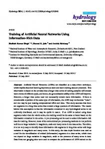
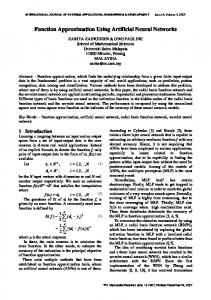
Here, (x, y) is the scalar product of the d dimensional vectors and nh is an arbitrary unit vector in the d dimensional space representing the normal vector of a selected hyperplane. If the point p is outside the convex hull of X, then its depth is 0. The convex hull of a set of points S is the smallest area polygon which encloses S. A formal example of convex hull is given in Figure 1. Points on and near the boundary have low depth, while points deep inside have a high depth. One advantage of this depth function is that it is invariant to affine transformations of the space. This means that the different ranges of the variable have no influence on their depth. The notion of the data depth function is not often used in the field of water resources. Chebana and Ouarda [36] used depth to identify the weights of a non-linear regression for flood estimation. Bárdossy and Singh [30] used the data depth function for parameter estimation of a hydrological model. Singh and Bárdossy [27] used the data depth function for the identification of critical events and developed the ICE algorithm. Recently, Singh et al. [31] used the data depth function for defining predictive uncertainty. Figure 1. Example of a convex hull.
Hyperplane
Hyperplane
8
A(Depth=0)
y
6
lowDepth
High Depth
2
4
B(Depth=4)
Convex Hull
2
4
6 x
8
10
Hydrology 2014, 1
45
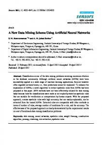
Figure 2. Flow chart for the identification of critical events (ICE) algorithm [29].
2.2. Identification of Critical Time Period Using the Data Depth Function The information content of the data can significantly influence the training of a data-driven model. Hence, if we can select only those data that are hydrologically reliable and are from a critical time period that has more variability, then we may improve our training process [32]. The ICE algorithm for the identification of critical events developed by [27] was used in this study. A flow chart for the ICE algorithm is given in Figure 2, where the example of event selection using discharge or the Antecedent Precipitation Index (AP I) is described. A brief description of the algorithm is given here. For details, please refer to [26,27]. To identify the critical time period that may contain enough information for identifying the model weights, unusual sequences in the series have to be identified. For simplicity, denote Xd (t) = (X(t − d + 1), X(t − d + 2), . . . , X(t)) for a given stage, discharge and sediment. For each t, the statistical depth Xd (t) with respect to the set Xd is calculated and denoted by D(t). The statistical depth is invariant to affine transformations. Depth can be calculated from untransformed
Hydrology 2014, 1
46
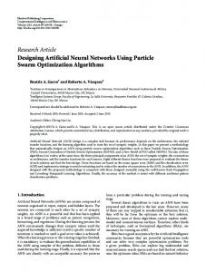
observation series of stage, discharge and sediment. Time steps t with a depth less than the threshold depth (D(t) < D0 ) are considered to be unusual. This is simply because unusual combinations in the multivariate case will cause a low depth. In practice, a more variable time period will have low depth, and it is useful for the identification of model weights. Such a set Xd for d = 2, calculated from the daily discharges, and the points with low depth are on the boundary of the convex hull, as shown in Figure 1. All of the points inside the convex hull have a higher depth. In this paper, critical events are defined around the unusual (low depth) days. A time t is part of a critical event if there is an unusual time t∗ in its neighbourhood defined as |t − t∗ | < δt . An example of events selected by using stage, discharge and sediment is given in Figure 3. Please note that the critical events are not only the extreme values in the series; instead, it is the combination of low flow, high flow, etc. Figure 3. Example of event selection. 20000 Event selection Observed Discharge EVENT 2 EVENT 1
Discharge(m3/s)
16000
12000
8000
4000
0 0
100
200
300
Time(Days)
3. Case Study The methodology presented in the last section will be demonstrated using ANN to construct a sediment rating curve. For the design and management of a water resources project, it is very much essential to know the volume of sediments transported by a river. It is possible to directly measure how much sediment is transported by the river, but not continuously. Consequently, a sediment rating curve is generally used. These curves can be constructed by several methods. In this regard, ANNs seem to be viable tools for fitting the relationship between river discharge and sediment concentration. 3.1. Artificial Neural Networks Artificial neural networks derive their central theme from highly simplified mathematical models of biological neural networks. ANNs have the ability to learn and generalize from examples to produce meaningful solutions to problems, even when the input data contains errors or is incomplete. They can also process information rapidly. ANNs are capable of adapting their complexity to model systems that
Hydrology 2014, 1
47
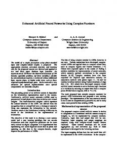
are non-linear and multi-variate and whose variables involve complex inter-relationships. Furthermore, ANNs are capable of extracting the relation between the input and output of a process without any knowledge of the underlying principles. Because of the generalizing capabilities of the activation function, one need not make any assumption about the relationship (i.e., linear or non-linear) between input and output. Since the theory of ANNs has been described in numerous papers and books, the same is described here in brief. A typical ANN consists of a number of layers and neurons; the most commonly used neural network in hydrology being a three-layered feed-forward network. The flow of data in this network takes place from the input layer to the hidden layer and then to the output layer. The input layer is the first layer of the network, whose role is to pass the input variables onto the next layer of the network. The last layer gives the output of the network and is appropriately called the output layer. The layer(s) in between the input and output layer are called hidden layer(s). The processing elements in each layer are called neurons or nodes. The numbers of nodes in input and output layers depends on the problem to be addressed and are decided before commencing the training. The number of hidden layers and the number of nodes in each hidden layer depend on the problem and the input data and are usually determined by a trial and error procedure. A synaptic weight is assigned to each link to represent the relative connection strength of two nodes at both ends in predicting the input-output relationship. The output of any node j, yj , is given as: ! m X yj = f Wi .Xi + bj (2) i=1
where Xi is the input received at node j, Wi is the input connection pathway weights, m is the total numbers of inputs to node j and bj is the node threshold. Function f is an activation function that determines the response of a node to the total input signal that is received. A sigmoid function is the commonly used activation function, which is bounded above and below, is monotonically increasing and is continuous and differentiable everywhere. The error back propagation algorithm is the most popular algorithm used for the training of feed-forward ANNs [38]. In this process, each input pattern of the training data set is passed through the network from the input layer to the output layer. The network output is compared with the desired target output, and an error is computed as: XX E= (yi − ti )2 (3) P
p
where ti is a component of the desired output T , yi is the corresponding ANN output, p is the number of output nodes and P is the number of training patterns. This error is propagated backward through the network to each node, and correspondingly, the connection weights are adjusted. Due to the boundation of the sigmoid function between zero and one, all input values should be normalized to fall in the range between zero and one before being fed into a neural network [39]. The output from the ANN should be denormalized to the original domain before interpreting the results. ASCE [38,40] contains a detailed review of the theory and applications of ANNs in water resources. Maier and Dandy [1] have also reviewed modeling issues and applications of ANNs for the prediction
Hydrology 2014, 1
48
and forecasting of hydrological variables. Maier et al. [41] have provided a state-of-the-art review of ANN applications to river systems. Govindaraju and Rao [42] have described many applications of ANNs to water resources. ANNs have been applied in the area of hydrology, including rainfall-runoff modeling [43–45], river stage forecasting [46–49], reservoir operation [50], describing soil water retention curves [51] and optimization or control problems [52]. ANN was employed successfully for predicting and forecasting hourly groundwater level up to some time ahead [53]. In a study, Cheng et al. [54] developed various ANN models with various training algorithm to forecast daily to monthly river flow discharge in Manwar Reservoir. A comparison of ANN model with a conventional method, like auto-regression, suggests that ANN provides better accuracy in forecasting. Other studies have also shown that ANNs are more accurate than conventional methods in flow forecasting and drainage design [55]. Furthermore, the ANN method was used extensively for the prediction of various variables (stream flow, precipitation, suspended sediment, etc.) in the water resources field [17,43,51,56–66]. Kumar et al. [67] found that an ANN model can be trained to predict lysimeter potential evapotranspiration values better than the standard Penman–Monteith equation method. Sudheer et al. [68] and Keskin and Terzi [69] tried to compute pan evaporation using temperature data with the help of ANN. Sudheer and Jain [70] employed a radial-basis function ANN to compute the daily values of evapotranspiration for rice crops. Trajkovic et al. [71] examined the performance of radial basis neural networks in evapotranspiration estimation. Kisi [72] studied the modelling of evapotranspiration from climatic data using a neural computing technique, which was found to be superior to the conventional empirical models, such as Penman and Hargreaves. Modelling of evapotranspiration with the help of ANN was also attempted by Kisi [73], Kisi and Öztürk [74] and Jain et al. [75]. Muttil and Chau [76] used ANN to model algal bloom dynamics. ANN has also been used in water quality modeling [77–79]. 3.2. Data Used in the Study The data used in this study was the same as used by [80]. For more details about the study area and data, please refer to [80]. Sufficiently long time series to obtain stable parameters from two gauging stations on the Mississippi River were available. Both stations are in Illinois and operated by the U.S. Geological Survey (USGS). These stations are located near Chester (USGS Station No. 07020500) and Thebes (USGS Station No. 07022000). The drainage areas at these sites are 1,835,276 km2 (708,600 mi2 ) for Chester and 1,847,190 km2 (713,200 mi2 ) at Thebes. For these stations, daily time series of river discharge and sediment concentration were downloaded from the web server of the USGS, and the river stage data were provided by USGS personnel. River discharge and sediment concentration were continuously measured at these sites for estimating the suspended-sediment discharge. For more details about the sites, the measurement procedures, etc., please refer to [81] and [82]. After examining the data and noting the periods in which there were gaps in one or more of the three variables, the periods for training and testing were chosen. For the Chester station, the data of 25 December 1985, to 31 August 1986, were chosen for training, and the data from 1 September 1986, to 31 January 1987, were chosen for testing. For the Thebes station, the data from 1 January 1990, to 30 September 1990, were used for
Hydrology 2014, 1
49
training, and data from 15 January 1991, to 10 August 1991, were used for testing. It may be noted that the periods from which training and testing data were chosen for the Thebes site span approximately the same temporal seasons (January–September and January–August). The data for the Chester site, however, covers slightly different months (i.e., December–August and September–January). Based on our experience on the use of very long time series or different time steps for the data, the results of the study are not expected to change. 3.3. Rating Curves and Input to ANN The records of stage can be transferred into records of discharge using a rating curve. Normally, a rating curve has the form: Q = a × Hb (4) where Q is discharge (m3 /s), H is river stage (m) and a and b are constant. The establishment of a rating curve is a non-linear problem. In a study, Jain and Chalisgaonkar [83] showed that ANN can represent the stage and discharge relation better than the conventional way, which uses Equation (4). A sediment rating curve has a very similar non-linear form as a discharge rating curve. Usually, the relationship is given by: S = c × Qd (5) where S is the suspended sediment concentration (mg/L), Q is discharge (m3 /s) and c and d are constant. Please note that establishing a sediment rating curve is a two-step process. The measured stage data are used to estimate discharge, and then, discharge is used to establish the sediment rating curve. Therefore, river stage, discharge and sediment concentration are the main inputs for analysis. The inputs to the ANN were river stages at the current and previous times. The other inputs were water discharge and sediment concentration at previous times. The input to the ANN model was standardized before applying ANN. The input was normalized by dividing the value with the maximum value to fall in the range [0, 1]. This ANN had two output nodes, one corresponding to water discharge and the other for sediment concentration. In a study, Jain [80] tried various combinations of input data of the stage, discharge and sediment concentration for the ANN model and found that the number of neurons in the hidden layer varies between two to 10. They suggest a network whose inputs are the current and previous stage; the discharge and sediment concentration of two previous periods can adequately map the current discharge and sediment concentration. Since the aim of this study was to test the feasibility of training the ANN model on critical events, we used the same setup of network as given by [80]. Hence, an integrated three-layer ANN, as described by Jain [80], was trained using the training period data pertaining to river stage, discharge and sediment concentration (Figure 4). The number of nodes in the hidden layer was determined based on the best correlation coefficient (CC) and the least root mean square (RMSE). Using the weights obtained in the training phase for each case, the performance of the ANN was checked by using the testing period data. Programs were developed in MATLAB 6.5 software using the neural network toolbox to pre-process the data, train the ANN and test it. The weights were obtained by the Levenberg–Marquardt algorithm, which is computationally efficient.
Hydrology 2014, 1
50
Input
Output
Figure 4. Three-layer, feed-forward ANN structure.
Input Layer
Hidden Layer
Output Layer
3.4. Different Cases for the Training of ANN To compare the training results of the ANN model on critical events with training on the whole data series, for each data set, the ANN model was trained and tested for three cases. The three different cases are given below. • Case 1: using the entire time series of data available, • Case 2: using the data pertaining to critical events only (selected by the depth function (ICE algorithm)), and • Case 3: using the data pertaining to randomly selected events (the same number of events as in Case 2). Here, a number of runs were taken by randomly selecting the events, and the results reflect the average of ten repetitions. 4. Results and Discussion Stage, discharge and sediment rating relations were determined for both sites using the ANN by following the same procedure as used by [80]. For both, the site river stage and discharge relationship was fitted using Equation (4); then, corresponding sediment discharge was computed using Equation (5). The ANN model was trained and tested on three different cases described in Section 3.5. RMSE and CC were used to test the results of the model in training and testing. RMSE accounts for the magnitude of the disagreement between the model and what is observed, whereas CC accounts for the disagreement in the dynamics of the model and what is observed. Tables 1 and 2 give the RMSE and correlation between the observed and the model for each case for the Chester site for the training and testing period, respectively. It can be seen from Table 1 that for discharge, the CC and RMSE are nearly the same for Cases 1 and 2; CC and RMSE for Case 3 are somewhat inferior. For the sediment concentration data, CC and RMSE were slightly inferior for Case 3. Testing results given in Table 2 show that for the discharge data, CC is very high and is nearly the same for Cases 1 and 2, whereas it is a “bit smaller” for Case 3; the RMSE is bit higher for Case 3. For the sediment data, CC is very high for Case 2 and is lower and nearly the same for Case 1 and 3; the RMSE is the best for Case 2, followed by Case 1, and worst for Case 3. In both the training and testing period, Case 3 has shown poor performance, as compared to Case 1 and 2 in terms of RMSE and CC. This shows that the random selection of events for training is not suitable for
Hydrology 2014, 1
51
training ANN models. This is simply because the random selection of an event does not represent the entire series, whereas critical events represent the whole series. Table 1. The RMSE and correlation coefficient for the ANN model for the training period for the Chester site. Cases
Discharge Correlation RMSE
Case 1 9.977×10⁻¹ Case 2 9.979×10⁻¹ Case 3 9.954×10⁻¹
1.330×10⁻² 1.503×10⁻² 2.309×10⁻²
Sediments Correlation RMSE 9.537×10⁻¹ 9.502×10⁻¹ 9.212×10⁻¹
% Data Used
6.116×10⁻² 7.823×10⁻² 7.908×10⁻²
100 53 53
Table 2. The RMSE and correlation coefficient for the ANN model for the testing period for the Chester site. Cases
Discharge Correlation RMSE
Case 1 9.928×10⁻¹ Case 2 9.904×10⁻¹ Case 3 9.670×10⁻¹
6.557×10⁻² 6.914×10⁻² 2.129×10⁻¹
Sediments Correlation RMSE 8.695×10⁻¹ 9.049×10⁻¹ 8.444×10⁻¹
7.874×10⁻² 6.859×10⁻² 1.225×10⁻¹
To aid the visual appraisal of the results, time series graphs were prepared. Figure 5 presents the observed and computed discharge for various cases for the Chester station for the testing period. The match is very good, except for the first and the major peak. Overall, the match is the best for Case 1 followed by Case 2 and Case 3, the difference between Case 1 and 2 being minor. Figure 6 presents the time series plot for the sediment data. Here, for some peaks and troughs, the graph for Case 1 is closer to what is observed, while for some others, the graph for Case 2 is closer. The graph for Case 3 appears to be consistently under performing. The time series plots for discharge and sediments for the ANN model based on Case 3 is inferior, both in timing, as well as in magnitude. Hence, it fails to represent the magnitude and dynamics of the series. These effect are coming from the use of randomly selected events, which may not have enough information for training the model. These figures affirm the interpretation of the results from Tables 1 and 2, that the ANN estimates by using the whole data and the ANN trained on critical events show a nearly similar match with the observed curve, whereas training by the random selection of events is inferior. Tables 3 and 4 give the RMSE and CC for the three cases for the Thebes site for the training and testing period, respectively. Results in Table 3 show that for discharge, the CC is very high and nearly the same for Cases 1 and 2, while it is a bit smaller for Case 3. The same can be said for RMSE, which is nearly twice for Case 3 compared to Case 2. Both CC and RMSE are inferior for Case 3. For sediment concentration data, CC is highest for Case 1, followed by Case 2 and then Case 3. The RMSE was very small for Case 1 and was almost the same for the remaining two cases.
Hydrology 2014, 1
52
Figure 5. Observed and computed discharge for each case for the Chester site testing period. 4
2.2
x 10
Observed case 1 case 2 case 3
2
1.8
Discharge (m3/s)
1.6
1.4
1.2
1
0.8
0.6
0.4
0.2
0
20
40
60
80 Time(days)
100
120
140
160
Figure 6. Observed and computed sediment concentration for each case for the Chester site testing period. 2500 Observed case 1 case 2 case 3
Sed. Concentration (mg/l)
2000
1500
1000
500
0
0
20
40
60
80 Time(days)
100
120
140
160
Testing results given in Table 4 show that for discharge, CC is very high and is nearly the same for Case 1 and 2; it was smaller for Case 3. The RMSE was quite high for Case 3, as compared to the other two cases. For the sediment data, the performance indices had a similar behaviour: CC was much less, and the RMSE was much high for Case 3 compared to the other two cases.
Hydrology 2014, 1
53
Table 3. The RMSE and correlation coefficient for the ANN model for the training period for the Thebes site. Cases
Discharge Correlation RMSE
Case 1 Case 2 Case 3
9.946e-01 9.929e-01 9.723e-01
2.137e-02 3.273e-02 6.034e-02
Sediments Correlation RMSE 9.045e-01 8.296e-01 7.425e-01
% Data Used
5.636e-02 1.023e-01 9.816e-02
100 29 29
Table 4. The RMSE and correlation coefficient for the ANN model for the testing period for the Thebes site. Cases
Discharge Correlation RMSE
Case 1 Case 2 Case 3
9.975e-01 9.949e-01 9.273e-01
Sediments Correlation RMSE
1.085e-02 2.226e-02 1.017e-01
9.439e-01 9.440e-01 8.984e-01
3.987e-02 4.049e-02 1.510e-01
Figure 7 shows the temporal variation of observed discharge and the estimates for all of the above three cases using ANN for the training period for the Thebes site. It can be appreciated from this figure that the graphs pertaining to Cases 1 and 2 are very close to the observed discharge curve, whereas the data for random events has been unable to train the ANN properly. A poorly-trained ANN fails in the test runs, as evidenced in Figure 8. These results are very similar to what we obtained for the Chester site. Figure 7. Observed and computed discharge for each case for the Thebes site testing period. 14000 Observed case 1 case 2 case 3 12000
Discharge (m3/s)
10000
8000
6000
4000
2000
0
50
100
150 Time(days)
200
250
Hydrology 2014, 1
54
Based on these results, it can be stated that the performance of ANN training using “information-rich” events is as good as that using the whole data set. At first glance, this statement may appear to challenge the widely repeated concept that an ANN becomes wiser as more data are used to train it. However, upon closer scrutiny, this concept supports the fact that if the data has multiple events that contain similar information about the natural system, then the ANN is not going to learn much despite spending a long time in training. Figure 8. Observed and computed sediment concentration for each case for the Thebes site testing period. 1800 Observed case 1 case 2 case 3
1600
Sed. Concentration (mg/l)
1400
1200
1000
800
600
400
200
0
0
50
100
150
200
Time(days)
Figure 9. Convex hull of the training and testing set. Inside points
D=0 Outside points D>0
Training data Validation data
250
Hydrology 2014, 1
55
Figure 10. Residuals of the observed and computed discharge at each testing period for the Chester site. 5000
Difference model and Observed Dis.
residual depth indicator
0.5 0
−5000
0
0
20
40
60
80 time (days)
100
120
140
Normalized Depth
1
160
Figure 11. Residuals of the observed and computed sediment concentration at each testing period for the Chester site. 1000
1 0.5 0
−1000
0
0
20
40
60
80 time (days)
100
120
140
160
Normalized Depth
Difference model and Observed Sedi.
residual depth indicator
Hydrology 2014, 1
56
The major limitation of the proposed method is the increase in pre-processing time of the data to select the information-rich data. However, one should note that we are using much less data (about half to one third) to achieve the same result compared to using the whole data set. Hence, in specific cases, for example, where we have missing series, we can achieve reasonable results. Training of any neural network is considered to be successful if the trained network works well on the testing data set. The analysis of results and the discussion presented above clearly show that the ANN trained on critical events has performed equally well for the tested data set. A model trained using a particular data set is likely to perform well on a test data set if both of the data sets are representative of the system and have similar features. A question arises as how to judge whether these data sets are similar or not. To test this, we did split sampling and divided the data into two sets, namely training and testing. We located the critical events as mentioned above, and the ANN was trained on the training data set. We validated the trained ANN on the testing set and calculated the depth of each data point of the testing set in the convex hull of the training set. Thus, we can locate which points of the testing set are in the convex hull of the training set. This practically means how similar the testing set with respect to the training set is. In a study, Bárdossy and Singh [84] have used a similar concept in the selection of an appropriate explaining variables for regionalization. Singh et al. [31] used a similar concept and developed the differentiating interpolation and extrapolation (DIE) algorithm to define predictive uncertainty. For visual appraisal of the concept, please refer to Figure 9. The space where the depth of any time step of testing data with respect to the convex hull of the training data is greater than zero means that the data have very similar properties as the training set, and one can expect less residuals and good performance. Figure 10 shows the residuals in the model and the observed discharge. In this figure, calculated depth is normalized and plotted along with the residual to indicate a depth equal to zero or higher for each time step with respect to the training data set. It can be appreciated from this figure that in the period where depth is zero, the residual is very high, and in the period where the depth is higher, the residual is lower. Similar results can be seen in the case of sediment data, as shown in Figure 11. This shows that the points that are inside the convex hull of the training set are the points where we can expect low errors. Practically, it shows that testing points that are in the convex hull of a training set are similar to the training set. Hence, one can predict or guess the performance of the model a priori by looking at the geometry of the training and testing data. 5. Summary and Conclusions Data from two gauging sites was used to compare the performance of ANN trained on the whole data set and just the data from critical events. Selection of data for critical events was done by two methods, using the depth function (ICE algorithm) and using random selection. Inter-comparison of the performance of the ANNs trained using the complete data sets and the pruned data sets shows that the ANN trained using the data from critical events, i.e., information-rich data, gave similar results as the ANN trained using the complete data set. However, if the data set is pruned randomly, the performance of the ANN degrades significantly. Thus, the selection of events by the depth function by following the method described by [26,27] is not only useful for a conceptual and a physically-based
Hydrology 2014, 1
57
model (as shown by previous studies [26,27,29,30]), but also for data-driven models. This strategy can result in substantial savings in time and effort in the training of models based on data-driven approaches, such as ANNs. For any DDMs, training data should have all possible events, which can describe the process well, irrespective of the length of the data set. There is always great effort and expertise needed to select the proper data set for the training. Therein lies the merit of the ICE algorithm, which automatically selects all of the possible combinations of events for training. In this study, the well-known back propagation algorithm for training neural networks was used, but the methodology can be used for other kinds of ANNs, such as radial basis function neural networks or support vector machines. This is due to the fact that the selection of information-rich data does not depend on the kind of the data-driven models being used. The concept of the paper can be used to predict the performance of the model a priori by looking at the geometry of the training and testing data. This in turn can be use to define the predictive uncertainty, as given by Singh et al. [31]. A possible criticism of the use of information-rich data could be that it may not result in substantial savings of time, since some time and effort will be spent in the identification of critical events. Note, however, that many runs of the ANN model have to be made in the typical case to determine the number of neurons in the hidden layer, etc. Moreover, it is felt that the chances of over fitting are less when data from information-rich events are used for training. There can be many unimportant input variables that may not contribute to the output. Hence, a limitation of the present study is that it does not make any selection of important inputs. The results of the present study may be further improved if a proper selection of input variables is made. The authors’ next work is in the same direction. The suggested methodology can be extended for the selection of input series among a large number of available input series. This may reduce the risk of feeding unnecessary or unimportant input series for training. Furthermore, the concept of this paper may be very useful for training data-driven models where the training time series is incomplete. However, further research is required to complete these task. Acknowledgments The work described in this paper was supported by a scholarship program initiated by the German Federal Ministry of Education and Research (BMBF) under the program of the International Postgraduate Studies in Water Technologies (IPSWaT) for the first author. Its contents are solely the responsibility of the authors and do not necessarily represent the official position or policy of the German Federal Ministry of Education and Research and the other organizations to which other authors belong. The authors would like to thank Xuanxuan Guan (editor) and two anonymous reviewers for many useful and constructive suggestions. Author Contributions All of the authors have made an equal contribution to this research. Conflicts of Interest The authors declare no conflict of interest.
Hydrology 2014, 1
58
References 1. Maier, H.R.; Dandy, G.C. Neural networks for the prediction and forecasting of water resources variables: A review of modelling issues and applications. Environ. Model. Softw. 2000, 15, 101–124. 2. Bowden, G.J.; Maier, H.R.; Dandy, G.C. Optimal division of data for neural network models in water resources applications. Water Resour. Res. 2002, 38, 1010. 3. Anctil, F.; Perrin, C.; Andréassian, V. Impact of the length of observed records on the performance of ANN and of conceptual parsimonious rainfall-runoff forecasting models. Environm. Model. Softw. 2004, 19, 357–368. 4. Bowden, G.J.; Dandy, G.C.; Maier, H.R. Input determination for neural network models in water resources applications. Part 1—Background and methodology. J. Hydrol. 2005, 301, 75–92. 5. Leahy, P.; Kiely, G.; Corcoran, G. Structural optimisation and input selection of an artificial neural network for river level prediction. J. Hydrol. 2008, 355, 192–201. 6. Nawi, N.M.; Atomi, W.H.; Rehman, M. The effect of data pre-processing on optimized training of artificial neural networks. Procedia Technol. 2013, 11, 32–39. 7. Marinkovi´c, Z.; Markovi´c, V. Training data pre-processing for bias-dependent neural models of microwave transistor scattering parameters. Sci. Publ. State Univ. NOVI Pazar Ser. A Appl. Math. Inform. Mech. 2010, 2, 21–28. 8. Gaweda, A.E.; Zurada, J.M.; Setiono, R. Input selection in data-driven fuzzy modeling. In Proceedings of the 10th IEEE International Conference of Fuzzy Systems (FUZZ-IEEE), Melbourne, VIC, Australia, 2–5 December 2001; Volume 1, pp. 2–5. 9. May, R.J.; Maier, H.R.; Dandy, G.C.; Fernando, T.M.K. Non-linear variable selection for artificial neural networks using partial mutual information. Environ. Model. Softw. 2008, 23, 1312–1326. 10. Fernando, T.M.K.G.; Maier, H.R.; Dandy, G.C. Selection of input variables for data-driven models: An average shifted histogram partial mutual information estimator approach. J. Hydrol. 2009, 367, 165–176. 11. Jain, A.; Maier, H.R.; Dandy, G.C.; Sudheer, K.P. Rainfall-runoff modeling using neural network: State-of-art and future research needs. ISH J. Hydraul. Eng. 2009, 15, 52–74. 12. Abrahart, R.J.; Anctil, F.; Coulibaly, P.; Dawson, C.W.; Mount, N.J.; See, L.M.; Shamseldin, A.Y.; Solomatine, D.P.; Toth, E.; Wilby, R.L. Two decades of anarchy? Emerging themes and outstanding challenges for neural network river forecasting. Progr. Phys. Geogr. 2012, 36, 480–513. 13. Cigizoglu, H.; Kisi, O. Flow prediction by three back propagation techniques using k-fold partitioning of neural network training data. Nordic Hydrol. 2005, 36, 49–64. 14. Wagener, T.; McIntyre, N.; Lees, M.J.; Wheater, H.S.; Gupta, H.V. Towards reduced uncertainty in conceptual rainfall-runoff modelling: Dynamic identifiability analysis. Hydrol. Process. 2003, 17, 455–476. 15. Chau, K.; Wu, C.; Li, Y. Comparison of several flood forecasting models in Yangtze River. J. Hydrol. Eng. 2005, 10, 485–491.
Hydrology 2014, 1
59
16. Chau, K.W.; Muttil, N. Data mining and multivariate statistical analysis for ecological system in coastal waters. J. Hydroinforma. 2007, 9, 305–317. 17. Wu, C.L.; Chau, K.W.; Li, Y.S. Methods to improve neural network performance in daily flows prediction. J. Hydrol. 2009, 372, 80–93. 18. Wu, C.L.; Chau, K.W.; Li, Y.S. Predicting monthly streamflow using data-driven models coupled with data-preprocessing techniques. Water Resour. Res. 2009, 45, W08432. 19. Wu, C.L.; Chau, K.W.; Fan, C. Prediction of rainfall time series using modular artificial neural networks coupled with data-preprocessing techniques. J. Hydrol. 2010, 389, 146–167. 20. Chen, W.; Chau, K. Intelligent manipulation and calibration of parameters for hydrological models. Int. J. Environ. Pollut. 2006, 28, 432–447. 21. Wu, C.; Chau, K.; Li, Y. River stage prediction based on a distributed support vector regression. J. Hydrol. 2008, 358, 96–111. 22. Wang, W.C.; Xu, D.M.; Chau, K.W.; Chen, S. Improved annual rainfall-runoff forecasting using PSO-SVM model based on EEMD. J. Hydroinform. 2013, 15, 1377–1390. 23. Jothiprakash, V.; Kote, A.S. Improving the performance of data-driven techniques through data pre-processing for modelling daily reservoir inflow. Hydrol. Sci. J. 2011, 56, 168–186. 24. Moody, J.; Darken, C.J. Fast learning in networks of locally-tuned processing units. Neural Comput. 1989, 1, 281–294. 25. Famili, F.; Shen, W.M.; Weber, R.; Simoudis, E. Data pre-processing and intelligent data analysis. Int. J. Intell. Data Anal. 1997, 1, 3–23. 26. Singh, S.K.; Bárdossy, A. Identification of critical time periods for the efficient calibration of hydrological models. Geophys. Res. Abstr. 2009, 11, EGU2009-5748. 27. Singh, S.K.; Bárdossy, A. Calibration of hydrological models on hydrologically unusual events. Adv. Water Resour. 2012, 38, 81–91. 28. Tukey, J. Mathematics and Picturing Data. In Proceedings of the 1974 International 17 Congress of Mathematics, Vancouver, BC, Canada, 21–29 August 1975; Volume 2, pp. 523–531. 29. Singh, S.K.; Liang, J.; Bárdossy, A. Improving the calibration strategy of the physically-based model WaSiM-ETH using critical events. Hydrol. Sci. J. 2012, 57, 1487–1505. 30. Bárdossy, A.; Singh, S.K. Robust estimation of hydrological model parameters. Hydrol. Earth Syst. Sci. 2008, 12, 1273–1283. 31. Singh, S.K.; McMillan, H.; Bárdossy, A. Use of the data depth function to differentiate between case of interpolation and extrapolation in hydrological model prediction. J. Hydrol. 2013, 477, 213–228. 32. Gupta, V.K.; Sorooshian, S. The relationship between data and the precision of parameter estimates of hydrologic models. J. Hydrol. 1985, 81, 57–77. 33. Rousseeuw, P.J.; Struyf, A. Computing location depth and regression depth in higher dimensions. Stat. Comput. 1998, 8, 193–203. 34. Liu, R.Y.; Parelius, J.M.; Singh, K. Multivariate analysis by data depth: Descriptive statistics, graphics and inference. Ann. Stat. 1999, 27, 783–858. 35. Zuo, Y.; Serfling, R. General notions of statistical depth function. Ann. Stat. 2000, 28, 461–482.
Hydrology 2014, 1
60
36. Chebana, F.; Ouarda, T.B.M.J. Depth and homogeneity in regional flood frequency analysis. Water Resour. Res. 2008, doi:10.1029/2007WR006771. 37. Dutta, S.; Ghosh, A.K.; Chaudhuri, P. Some intriguing properties of Tukey’s half-space depth. Bernoulli 2011, 17, 1420–1434. 38. ASCE Task Committee on Application of Artificial Neural Networks in Hydrology. Artificial neural networks in hydrology, I: Preliminary concepts. J. Hydrol. Eng. 2000, 5, 115–123. 39. Smith, J.; Eli, R.N. Neural network models of rainfall-runoff process. J. Water Resour. Plan. Manag. 1995, 121, 499–508. 40. ASCE Task Committee on Application of Artificial Neural Networks in Hydrology. Artificial neural networks in hydrology, II: Hydrological applications. J. Hydrol. Eng. 2000, 5, 124–137. 41. Maier, H.; Jain, A.; Dandy, G.; Sudheer, K.P. Methods used for the development of neural networks for the prediction of water resource variables in river systems: Current status and future directions. Environ. Model. Softw. 2010, 25, 891–909. 42. Govindaraju, R.S.; Rao, A. Artificial Neural Networks in Hydrology; Kluwer Academic Publishers: Dordrecht, The Netherlands, 2000. 43. Cigizoglu, H.K. Estimation, forecasting and extrapolation of river flows by artificial neural networks. Hydrol. Sci. J. 2003, 48, 349–361. 44. Wilby, R.L.; Abrahart, R.J.; Dawson, C.W. Detection of conceptual model rainfall-runoff processes inside an artificial neural network. Hydrol. Sci. J. 2003, 48, 163–181. 45. Lin, G.F.; Chen, L.H. A non-linear rainfall-runoff model using radial basis function network. J. Hydrol. 2004, 289, 1–8. 46. Imrie, C.E.; Durucan, S.; Korre, A. River flow prediction using artificial neural networks: Generalization beyond the calibration range. J. Hydrol. 2000, 233, 138–153. 47. Lekkas, D.F.; Imrie, C.E.; Lees, M.J. Improved non-linear transfer function and neural network methods of flow routing for real-time forecasting. J. Hydroinforma. 2001, 3, 153–164. 48. Shrestha, R.R.; Theobald, S.; Nestmann, F. Simulation of flood flow in a river system using artificial neural networks. Hydrol. Earth Syst. Sci. 2005, 9, 313–321. 49. Campolo, M.; Soldati, A.; Andreussi, P. Artificial neural network approach to flood forecasting in the River Arno. Hydrol. Sci. J. 2003, 48, 381–398. 50. Jain, S.K.; Das, A.; Srivastava, D.K. Application of ANN for reservoir inflow prediction and operation. J. Water Resour. Plan. Manag. ASCE 1999, 125, 263–271. 51. Jain, S.K.; Singh, V.P.; van Genuchten, M. Application of ANN for reservoir inflow prediction and operation. J. Water Resour. Plan. Manag. ASCE 2004, 9, 415–420. 52. Bhattacharya, B.; Lobbrecht, A.H.; Solomatine, D.P. Neural networks and reinforcement learning in control of water systems. J. Water Resour. Plan. Manag. ASCE 2003, 129, 458–465. 53. Taormina, R.; Chau, K.W.; Sethi, R. Artificial neural network simulation of hourly groundwater levels in a coastal aquifer system of the Venice Lagoon. Eng. Appl. Artif. Intell. 2012, 25, 1670–1676. 54. Cheng, C.; Chau, K.; Sun, Y.; Lin, J. Long-term prediction of discharges in Manwan reservoir using artificial neural network models. Lect. Notes Comput. Sci. 2005, 3498, 1040–1045.
Hydrology 2014, 1
61
55. Zealand, C.M.; Burn, D.H.; Simonovic, S.P. Short term streamflow forecasting using artificial neural networks. J. Hydrol. 1999, 214, 32–48. 56. Tokar, A.S.; Johnson, P.A. Rainfall-runoff modelling using artificial neural networks. J. Hydrol. Eng. 1999, 4, 232–239. 57. Cigizoglu, H.K. Estimation and forecasting of daily suspended sediment data by multi layer perceptrons. Adv. Water Resour. 2004, 27, 185–195. 58. Sudheer, K.P.; Jain, A. Explaining the internal behaviour of artificial neural network river flow models. Hydrol. Process. 2004, 18, 833–844. 59. Kumar, A.R.S.; Sudheer, K.P.; Jain, S.K. Rainfall-runoff modeling using artificial neural networks: Comparison of network types. Hydrol. Process. 2005, 19, 1277–1291. 60. Cigizoglu, H.K.; Kisi, O. Flow prediction by three back propagation techniques using k-fold partitioning of neural network training data. Nordic Hydrol. 2005, 361, 1–16. 61. Cigizoglu, H.K.; Kisi, O. Methods to improve the neural network performance in suspended sediment estimation. J. Hydrol. 2006, 317, 221–238. 62. Cigizoglu, H.K.; Alp, M. Generalized regression neural network in modelling river sediment yield. Adv. Eng. Softw. 2006, 372, 63–68. 63. Lin, J.; Cheng, C.T.; Chau, K.W. Using support vector machines for long-term discharge prediction. Hydrol. Sci. J. 2006, 51, 599–612. 64. Alp, M.; Cigizoglu, H.K. Suspended sediment estimation by feed forward back propagation method using hydro meteorological data. Environ. Model. Softw. 2007, 22, 2–13. 65. Solomatine, D.; Ostfeld, A. Data-driven modelling: Some past experiences and new approaches. J. Hydroinform. 2008, 10, 3–22. 66. Shamseldin, A. Artificial neural network model for river flow forecasting in a developing country. J. Hydroinform. 2010, 12, 22–35. 67. Kumar, M.; Raghuwanshi, N.S.; Singh, R.; Wallender, W.W.; Pruitt, W.O. Estimating evapotranspiration using artificial neural network. J. Irrig. Drain. Eng. ASCE 2002, 128, 224–233. 68. Sudheer, K.P.; Gosain, A.K.; Rangan, D.M.; Saheb, S.M. Modeling evaporation using artificial neural network algorithm. Hydrol. Process. 2002, 16, 3189–3202. 69. Keskin, M.E.; Terzi, O. Artificial Neural Network models of daily pan evaporation. J. Hydrol. Eng. 2006, 11, 65–70. 70. Sudheer, K.P.; Jain, S.K. Radial basis function neural networks for modelling rating curves. J. Hydrol. Eng. 2003, 8, 161–164. 71. Trajkovic, S.; Todorovic, B.; Stankovic, M. Forecasting reference evapotranspiration by artificial neural networks. J. Irrig. Drain. Eng. 2003, 129, 454–457. 72. Kisi, O. Evapotranspiration modeling from climatic data using a neural computing technique. Hydrol. Process. 2007, 21, 1925–1934. 73. Kisi, O. Generalized regression neural networks for evapotranspiration modeling. J. Hydrol. Sci. 2006, 51, 1092–1105. 74. Kisi, O.; Öztürk, O. Adaptive neurofuzzy computing technique for evapotranspiration estimation. J. Irrig. Drain. Eng. 2007, 133, 368.
Hydrology 2014, 1
62
75. Jain, S.K.; Nayak, P.C.; Sudheer, K.P. Models for estimating evapotranspiration using artificial neural networks, and their physical interpretation. Hydrol. Process. 2008, 22, 2225–2234. 76. Muttil, N.; Chau, K.W. Neural network and genetic programming for modelling coastal algal blooms. Int. J. Environ. Pollut. 2006, 28, 223–238. 77. Zhang, Q.; Stanley, S.J. Forecasting raw-water quality parameters for the North Saskatchewan River by neural network modeling. Water Res. 1997, 31, 2340–2350. 78. Palani, S.; Liong, S.Y.; Tkalich, P. An ANN application for water quality forecasting. Marine Pollut. Bull. 2008, 56, 1586–1597. 79. Singh, K.P.; Basant, A.; Malik, A.; Jain, G. Artificial neural network modeling of the river water quality—A case study. Ecol. Model. 2009, 220, 888–895. 80. Jain, S.K. Development of integrated sediment rating curves using ANNS. J. Hydraul. Eng. 2001, 127, 30–37. 81. Porterfield, G. Computation of fluvial-sediment discharge. In Techniques of Water-Resources Investigations of the United States Geological Survey; US Government Printing Office: Washington, DC, USA, 1972; Chapter C3; pp. 1–66. 82. USGS Sediment Data Portal. Available online: http://co.water.usgs.gov/sediment/introduction.html (accessed on 30 September 2009). 83. Jain, S.K.; Chalisgaonkar, D. Setting up stage-discharge relations using ANN. J. Hydrol. Eng. 2000, 5, 428–433. 84. Bárdossy, A.; Singh, S.K. Regionalization of hydrological model parameters using data depth. Hydrol. Res. 2011, 42, 356–371. c 2014 by the authors; licensee MDPI, Basel, Switzerland. This article is an open access article
distributed under the terms and conditions of the Creative Commons Attribution license (http://creativecommons.org/licenses/by/3.0/).