doi: 10.5028/jatm.v10.948
ORIGINAL PAPER
xx/xx
Trajectory Optimization of Launch Vehicles Using Object-oriented Programming Fábio Antônio da Silva Mota1, José Nivaldo Hinckel2, Evandro Marconi Rocco2, Hanfried Schlingloff3 How to cite Mota FAS
http://orcid.org/0000-0003-3672-0547
Hinckel JN
http://orcid.org/0000-0002-0171-2697
Rocco EM
http://orcid.org/0000-0003-0660-0587
Schlingloff H
Mota FAS; Hinckel JN; Rocco EM; Schlingloff H (2018) Trajectory Optimization of Launch Vehicles Using ObjectOriented Programming. J Aerosp Technol Manag, 10: e3918. doi: 10.5028/jatm.v10.948.
http://orcid.org/0000-0003-1806-9113
ABSTRACT: The aim of this study is to model launch vehicles with focus on 3-DOF trajectory optimization using a modular approach. Despite the large number of operational launch vehicles, they usually consist of basic components and subsystems. In other words, a launch vehicle is an assembly of stages, which in turn is divided into propellant system and engine, and the engine is an assembly of basic components such as pumps, turbines, combustion chamber, and nozzle. To allow future extension and reuse of the codes, a modular structure using object-oriented programming is used. Two formulations of state equations of the trajectory and two optimization methods are described. The launch vehicle performance will be measured by payload mass for a given mission. The simulations of the VLS-1, Ariane 5 and VLS-Alfa were performed and showed good agreement with the literature. KEYWORDS: Launch vehicle, Trajectory, Optimization, Object-oriented programming.
INTRODUCTION Due to the inherent complexity of a launch vehicle, its design is traditionally divided into multiple disciplines, such as trajectory optimization, propulsion, aerodynamics, and mass budget. Despite the large number of operational launch vehicles, they usually consist of basic components. In other words, a launch vehicle is an assembly of stages, which in turn is divided into propellant system and engine, and the engine is an assembly of basic components such as pumps, turbines, combustion chamber, and nozzle (for a liquid rocket stage). Space launch systems are composed by a large number of components grouped into a hierarchy of subsystems. The performance of the vehicle depends on the individual performance of each of the subsystems, which in turn depend on material properties and design parameters. Changes in design parameters are propagated throughout the cluster hierarchy of subsystems and components, flight trajectory and payload capability (Hinckel 1995). In order to get the best performance of a given launch vehicle, and consequently, to make the access to space less costly, trajectory optimization techniques have been for decades a subject of intense research. Trajectory optimization can be categorized basically into direct and indirect methods. Betts (1998) and Rao (2009) have made a comprehensive discussion about both methods. The reason for this method to be called “indirect” comes from the strategy to convert the original optimal control problem into a boundary-value problem. The most common indirect methods found in the literature are the shooting method,
1.Universidade Federal do ABC – Centro de Engenharia, Modelagem e Ciências Sociais Aplicadas – Departamento de Engenharia Aeroespacial – Santo André/ SP – Brazil. 2.Instituto Nacional de Pesquisas Espaciais – Departamento de Engenharia e Tecnologia Espacial – São José dos Campos/SP – Brazil. 3.Ostbayerische Technische Hochschule Regensburg – Department of Mechanical Engineering – Regensburg – Germany. Correspondence author: Fábio Antônio da Silva Mota | Universidade Federal do ABC – Centro de Engenharia, Modelagem e Ciências Sociais Aplicadas – Departamento de Engenharia Aeroespacial | Av. dos Estados, 5001 | CEP: 09210-580 – Santo André/SP – Brazil | E-mail:
[email protected] Received: Jun. 8, 2017 | Accepted: Nov. 6, 2017 Section Editor: Luiz Martins-Filho
J. Aerosp. Technol. Manag., São José dos Campos, v10, e3918, 2018
02/15 xx/xx simple
method to evaluate the performance of multistage launch vehicles for given
Mota FAS; Hinckel JN; Rocco EM; Schlingloff H
structural data, aerodynamic and propulsive parameters. the multiple-shooting method, and collocation methods (Brown et al. 1969; Teren and Spurlock 1966; Miele and Wang 2003). The purpose work is to develop tool, which can be easilyanalysis, reused Presumably because of the possibilityofof this solving complex problems with a a minimum effort of mathematical theand direct method is the one chosen by most researchers (Hargraves and Paris 1987; Seywald 1994; Herman and Conway 1996; Balesdent extended, model andused simulate a launch vehicle with focus trajectory. Thus, the 2011). One of the mostto popular software extensively in many publications is called POSTon (Program to Optimize Simulated Trajectories) (Brauer et al. 1977). POST is a commercial program that has been used successfully to solve a wide variety of toolascent is intended be capable modeling and flight trajectory orbit atmospheric and reentryto problems, as well asof exoatmospheric orbitaloptimizing transfer problems. In the framework until of this method, the problem is characterized by a set of parameters that define the control law. This problem is a typical Non Linear Programming mathematical models formethods determination ofmethods) performance of a launch Problem injection. (NLP) and canTwo be solved using classical Gradient-based (deterministic such as Sequential Quadratic Program (SQP) or by heuristic methods. According to Betts (1998), heuristic optimization algorithms are not computationally vehicle will methods. be described andpresumably discussed. vehiclewithout performance will be competitive with gradient Even though due toThe ease oflaunch implementation a detailed understanding of the system, in the last two decades lots of papers using Particle Swarm Optimization (PSO), genetic algorithms (GA), among measured payload for a given mission. others were applied toby solve trajectorymass optimization problems. As for indirect methods, the direct methods can be categorized in direct (multiple) shooting or collocation. In the case where only the control variables are adjusted by a function, the method TRAJECTORY MODELING is called a shooting method. When both the state and control are parameterized, the method is called a collocation method. A well-known software developed by the University of Stuttgart, which addresses the direct collocation method, is the AeroSpace SinceSoftware the dawn of the space era launch vehicles are responsible to put satellites Trajectory Optimization (ASTOS). For either direct or indirect approaches, perhaps the most important benefit gained from a multiple shooting formulation This makes the iscost of arobustness. satellite To strongly related to the performance of the a comparedinto to itsorbit. precursor (single shooting) enhanced take advantage of both methods previously described, hybrid method can also be considered (von Stryk and Bulirsch 1992; Pontani and Teofilatto 2014; Gath and Calise 2001). The idea launch vehicle, which in turn depends ondistinct the trajectory profile. behind this approach is to divide the flight trajectory into two phases, namely atmospheric and exoatmospheric phases, applying the direct method in the first phase and indirect method in the second one. Here, exoatmospheric phase means that the Atmosphere ModelPontani and Teofilatto (2014) proposed a simple vehicle is virtually in vacuum space, i.e., the aerodynamic effects can be ignored. method to evaluate the performance of multistage launch vehicles for given structural data, aerodynamic and propulsive parameters. atmosphere seen a layer gases attached surface of vehicle the The purpose ofThe this work is to develop can a tool,be which can as be easily reusedofand extended, to modelto andthe simulate a launch with focus on trajectory. Thus, the tool is intended to be capable of modeling and optimizing flight trajectory until orbit injection. Earth bymodels gravitational attraction. This work makes the standard atmosphere, Two mathematical for determination of performance of a launch vehicleuse will of be described and discussed. The launch vehicle performance will be measured by payload mass for a given mission.
which is modeled as adjacent layers of gases in which temperature depends on the
altitude. InMODELING different layers, the temperature can be modeled as linear function of the TRAJECTORY Sincealtitude. the dawn of the space era launch vehicles are responsible to put satellites into orbit. This makes the cost of a satellite strongly related to the performance of the launch vehicle, which in turn depends on the trajectory profile.
Aerodynamics
ATMOSPHERE MODEL theasflight, launch vehicle needsofto thegravitational atmosphere in which reacts The atmosphereDuring can be seen a layer ofagases attached to the surface thecross Earth by attraction. This work makes use of the standard atmosphere, which is modeled as adjacent layers of gases in which temperature depends on the altitude. In thethevehicle motion means of aerodynamics forces. The drag force arises due to different to layers, temperature can be by modeled as linear function of the altitude.
friction between the body and the fluid (Eq. 1): AERODYNAMICS During the flight, a launch vehicle needs to cross the atmosphere in which reacts to the vehicle motion by means of aerodynamics forces. The drag force arises due to friction between the body and the fluid (Eq. 1): D=
J. Aerosp. Technol. Manag., São José dos Campos, v10, e3918, 2018
1 r (r ) SC DV 2 2
(1)
(1)
5
combustion of the propellants and for liquid rocket engines there 3is still the sloshing, where: D = drag force (N); ρ = density of the working fluid (kg/m ); S = reference area Trajectory Optimization of Launch Vehicles Using Object-oriented Programming combustion of the propellants for the liquid rocket engines is still the sloshing, 03/15 xx/xx which is the movement of fluid and within tanks and pipes andthere rotating equipment such (m2); CD = drag coefficient (–); and V = air speed (m/s).
combustion of the propellants for liquid rocket engines still the sloshing, which is theand movement ofEspecially fluidand within tanks and pipes andthere rotating equipment as turbines pumps. forthe large launch vehicles, theis deflection of such the
lift isρ a= reaction force to the angle of 3 attack (Eq. 2): where:combustion D = dragThe forceof (N); density of the working (kg/m ); S = reference (m2);isCDstill = drag (–); and the propellants and forfluid liquid rocket enginesarea there thecoefficient sloshing, V = structure air speed (m/s). which is should the and movement ofEspecially fluidaswithin thelarge tankslaunch and and rotating equipment as turbines the deflection ofsuch the bepumps. considered wellfor (Cornelisse et pipes al.vehicles, 1979). However, this research The lift is a reaction force to the angle of attack (Eq. 2): which is the movement of fluid within the tanks and pipes and rotating equipment such
as focused turbines pumps. Especially largetreatment launch the deflection of the should considered as wellfor(Cornelisse et al.vehicles, However, this research isstructure onand thebe reference trajectory, thus of1979). the translational motion is (2) 1 2 L = large r (r )SC as turbines and pumps. Especially for launch vehicles, the deflection of the (2) LV 2 structure bethis considered as mathematical well (Cornelisse et al.for 1979). However,are thispresented research is focusedshould the reference trajectory, thus treatment of the trajectory translational motion is sufficient to on fulfill task. Two models the structure should be considered2 as well (Cornelisse et al. 1979). However, this research where: = lift forceto(N); Sthe = reference area (m ); CLmathematical coefficient (–); and V =for air speed (m/s). is focused on reference trajectory, thus of translational sufficient fulfill this task. Two models the trajectory are motion presented in Lthe following sections. The first= lift one was treatment taken from Schlingloff (2005) and theis 2 where: L methods = lift force (N);the S =aerodynamic referencecoefficients area (min );theCliterature, (–); tool andMissile V = air L = lift coefficient There are many to estimate i.e., the well-known DATCOM, is focused on the reference trajectory, thus treatment of the translational motion is interpolation offollowing available datasections. from atask. givenThe vehicle, closed formulas that consider contributions of shock wave inand the rocket nose, sufficient to fulfill this Two mathematical models for the trajectory are presented in the first one was taken from Schlingloff (2005) the second one from Tewari (2007). speedand (m/s). body friction base pressure, or even constant value for certain phases of the flight. Except for interpolation from real flight sufficient to fulfill this task. Two mathematical models for the trajectory are presented data,in the methods estimate the drag (2007). coefficient are quite inaccurate. Fortunately, the essential(2005) acceleration the following sections. The first one was taken frombecause Schlingloff andphase thebegins second oneto from Tewari First Formulation Therephase, areusually many methods estimate the performance aerodynamic coefficients in the in the exoatmospheric the drag has little to influence on launcher (Schlingloff 2005). in the following sections. The first one was taken from Schlingloff (2005) and the secondIn onethis from Tewari (2007). First Formulation formulation, the spherical celestial (inertial) coordinates and a moving literature, i.e.,TRANSLATIONAL the well-knownMOTION tool Missile DATCOM, interpolation of available data EQUATIONS OF THE second one from Tewari (2007). The modeling of the trajectory of a launch vehicle is usually performed by means of two reference frames (one with origin on First Formulation In this formulation, spherical celestial moving coordinates in the orbit planethe were considered. Both (inertial) referencecoordinates frames haveand the aorigin on the Earth center and the other one moving the vehicle) andconsider considerations or idealizationsofaccording the requirements from a given vehicle, closedwith formulas that contributions shock to wave in the First Formulation of the mission. To model the translational motion, the vehicle can be treated as a particle, ignoring the size and mass distribution. In this formulation, the spherical celestial coordinates and moving coordinates in the orbit plane were considered. Both(inertial) reference frames have theaas origin the Earth center (Fig. 1). The vector of state variables is conveniently chosen y(t) on = In modeling thenose, rotational motion, the vehicle can bepressure, consideredor a rigid body, reducingvalue the degrees of freedom from infinity rocket body friction and base even constant for certain phases of In this formulation, the spherical celestial (inertial) coordinates and a moving (flexible body case) to just six (Tewari 2007). Strictly speaking, a launch vehicle is far from being considered a rigid body. Mass is T were coordinates inΩ(t) the(Fig. orbit plane considered. Both reference have the origin the Earth center 1). The vector variables isofconveniently chosen as y(t)on [r(t) u(t) v(t) ι(t) ω(t)] , ofwhere: Ωof= state rightfor ascension theframes ascending node (rad); ω= is the continuously expelledExcept due to combustion the propellants liquid rocket engines is still the which the flight. for interpolation fromandreal flight data, the there methods tosloshing, estimate the coordinates in the orbit plane were considered. Both reference frames have the origin on movement of fluid within the tanks and Tpipes and rotating equipment such as turbines and pumps. Especially for large launch the Earth center (Fig. 1).(rad); The vector state isof conveniently chosen as y(t) ω = u(t) v(t) ι(t) ω(t)] , where: rightvariables ascension the ascending node (rad); =[r(t) argument ofΩ(t) periapsis and TΩof ==temperature (K). Thus, the system of research equation vehicles, the deflection of the are structure should be considered as well (Cornelisse et al. 1979). thisacceleration is focused drag coefficient quite inaccurate. Fortunately, because the However, essential Earthtrajectory, center thus (Fig. 1). The vector of state variables is conveniently chosen as y(t) = on thethe reference treatment T of the translational motion is sufficient to fulfill this task. Two mathematical models [r(t) u(t) v(t) Ω(t) ι(t) ω(t)] , where: right ascension the ascending (rad); ω = argument of periapsis (rad); and TΩ==temperature (K).ofThus, the systemnode of equation cantrajectory be given (Eqs. 3-9): for the areas presented the following sections. The firstusually one was the takendrag from Schlingloff and the on second phase begins in thein exoatmospheric phase, has little(2005) influence T [r(t) u(t) v(t) Ω(t) ι(t) ω(t)] , where: Ω = right ascension of the ascending node (rad); ω one from Tewari (2007). = argument (rad); and T = temperature (K). Thus, the system of equation can be givenof as periapsis (Eqs. 3-9): launcher performance (Schlingloff 2005). argument of periapsis (rad); and T = temperature (K). Thus, the system of equation First = Formulation can be given as (Eqs. 3-9): r! = u (3) In this formulation, the spherical celestial (inertial)ofcoordinates and a moving coordinates Equations the Translational Motion in the orbit plane were considered. be given (Eqs. 3-9):on the Earth center (Fig. 1). The vector of state variables is conveniently chosen as Both can reference frames as have the origin r! = u (3) of T y(t) = [r(t) u(t) v(t) Ω(t)modeling ι(t) ω(t)] , where = vertical velocity of (m/s); = horizontal velocityis(m/s); where:performed Ω = right ascension The of uthe trajectory a vlaunch vehicle usually by 2 (4) D x ofLequation µ (rad). v periapsis F Thus, the system the ascending node (rad) and ω = argument of can be given as (Eqs. 3-9): x u! = + sin + r! =bucos d + (3) r r2 m m m means of two reference frames (one with origin on the Earth center and the other one 2 (4) ! D L µ F r =u v (3) (3) u! = + sin b cos d + x + x r
2
m
m
m
r moving with the vehicle) vand considerations or according to (4) the 2 D idealizations L µ F u! = - 2 + sin b cos d + x + x (5) Dy m (4) D Ly m L vr 2µv r µF mF cos sin bthe cos dtranslational +d + +x + x motion, the vehicle can be requirements of the mission. uv! = -To- +model + b cos 2 m mm m rr rm m (5) Dy Ly µv F v! = the - size + cos bmass cos d +distribution. + treated as a particle, ignoring and In modeling the rotational r m m m (5) Dy Ly µv F =+ cos brigid cos d body, + +reducing the degrees of freedom motion, the vehicle can bev! considered a (6) (5) Dy m Ly rµv W m m !F= w sin w
(4)
(5)
(6) cosx bsin cosi d + + m m m from infinity (flexible body case) to just (Tewari 2007). Strictly speaking, a launch w (6) ! = wsixsin W x i! = w x cos (7) (7) sinwi vehicle is far from being considered a! rigid sin body. w Mass is continuously expelled due (6)to W = wx v 7 2018 sin sinwiwcot i J. Aerosp. Technol. Manag., São José dos Campos, v10,(8) (6) e3918, w! = W ! - w x sin 6 r = w x sin i
v! = -
r
+
7
04/15 xx/xx
Mota FAS; Hinckel JN; Rocco EM; Schlingloff H
i! = w x cos w
(7)
v
(8) (7)
w! = i! -=w x sin w cot i r w x cos w v - w x sin w cot i r
wx =
F sin d + D z + L z v
(9)
F sin d + D + L
(9)
and and
(8)
w! =
(8)
(9)
z plane z where: β = thrust angle in flight plane (rad); δ = thrust out of flight (rad); and F = thrust force (N); ωx = inclination w x angle = v where: β = thrust angle in flight plane (rad); δ = thrust angle out of flight plane (rad); and F = change (rad). Equations 3 to 5 of the system of differential equations are the dynamic equations of motion and Eqs. 6 to 9 are the kinematic thrust force (N); ωx = inclination change (rad). equations. The dynamic equations are derived by application of the Newton’s Second Law resolved into components of the moving where: β = thrust angle in flight plane (rad); δ = thrust angle out of flight plane (rad); and F = system. The kinematic equations are deducted into two steps: representation of the rotation velocity of the vehicle in a vector form, and applying Euler(N); angles 2005). thrusttheforce ω (Schlingloff = inclination change (rad). x
z
ZI y
Actual flight plane
v x
ω Ω XI
ι
YI
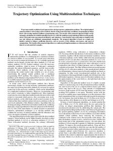
Figure 1. Reference Frames. Figure 1. Reference frames.
Second Formulation 1. Reference Frames. equations are the dynamic Equations 3 to 5 of Figure the system of differential The reference frames adopted in this modeling are the planet-fixed reference (SXYZ) frame and the local horizontal frame (oxyz), equations both are non-inertial (Fig.and 2). Eqs. 6 to 9 are the kinematic equations. The dynamic equations of motion
Equations 3 to 5 of the system of differential equations are the dynamic are derived by application of the Newton’s ZSecond Law resolved into components of the equations of motion and Eqs. 6 to 9 are the kinematicγ equations. y (cast)The dynamic equations z (north) x (up)representation of moving system. The kinematic equations are deducted into two steps: are derived by application of the Newton’s Second Law resolved into components of the the rotation velocity of the vehicle in a vector form, and applying the Euler angles o moving system. The kinematic equations are deducted into two steps: representation of r Equator (Schlingloff 2005). the rotation velocity of the vehicle in aS vector ϕform, and applying the Euler angles Y Second Formulation (Schlingloff 2005). ξ The reference frames adopted in this modeling are the planet-fixed reference Second Formulation (SXYZ) frame and the localXhorizontal frame (oxyz), both are non-inertial (Fig. 2). The reference frames adopted in this modeling are the planet-fixed reference Figure 2. Planet-fixed and local horizon frames for atmospheric flight (adapted from Tewari 2007).
(SXYZ) frame and the local horizontal frame (oxyz), both are non-inertial (Fig. 2). J. Aerosp. Technol. Manag., São José dos Campos, v10, e3918, 2018
8
8
ORIGINAL PAPER ORIGINALPAPER PAPER ORIGINAL ORIGINAL PAPER ORIGINAL PAPER
v = r!i + Ω ´ (ri)
(13)
Trajectory Optimization of Launch Vehicles Using Object-oriented Programming
v = r!i + rx! cosfj + rf!k
05/15 xx/xx (14)
From Fig. 2, the relative velocity v and the local velocity of the local horizontal frame (oxyz) relative to the planet-centered v = r!i + Ω ´ (ri) (13) rotating frame (SXYZ) can be expressed as and v(v13 , (Eqs. ,and ) =10 v (sin i + cos obtain sin j +the coskinematic cos k ) equations of(10) Comparing Eqs. 14 we11): finally motion
(Eqs. 15-17):
(sin ii++cos cossin sin jj++cos coscos cos kk)) vv((vv,,,,))==vv(sin v =r!ii + x! cos fj + rjf!+k cos cos k ) v(v, , ) = v (sin + rcos sin v(v, , ) = v (sin i + cos sin j + cos cos k )
(10) (10) (10) (14) (10)
(1) Ω = K − j v sin =K gjj (1) (15) (1) Ω==r! K −− Ω v =Ωr!i=+ΩK´−(ri) j (1) (13) Comparing Eqs. 13 and 14 we finally Kobtain j the kinematic equations of motion (1) = − Ω where: γ = flight path angle (rad); ζ = heading angle (= π/2 – A); and ξ =zlongitude (rad); and A = azimuth (rad). v cos g cos (16) ! x =!only ! sin inj +terms !cosofaxes (12) i − k With a convenient rotation matrix, Eq. 11 canΩvbe= written of the body as (Eq. 12): (14) j + rfk = ri + rx cosrfcos (Eqs. 15-17): jj++f coskk sin Ω (12) (12) Ω== sin − Ω v =ri!ii−+ ´ (ricos ) (13) (12) Ω = sin jj´++(ricos (12) (13) v =!ri!i−+ Ω )coskk Ω = sin − r = v sin g (15) ! cosg fcos (14) v = r!!i + rvxcos j + zrf!k (17) f = 14): ! (14) The relativeComparing velocity can also be expressed as (Eqs. 13 Eqs. 13 and 14 wevfinally the kinematic equations of motion i +v rcos x!obtain f j f k = r!and cos + r r z g cos (16) xv! = r i + Ω (r i) (13) r cos Ωf((rrii)) (13) vv==rrii++Ω (13) (Eqs. 15-17): v = r i + Ω ( r i ) (13) =v rfinally i=+rrNewton’s (jr+i)rSecond the k kinematic i+cos Ωobtain Comparing Eqs. 13 and equations 14vwe equations of (14) motion (13) To derive the dynamic Law must be introduced (14) (Eq. (14) = r + r cos + r v i j k = r + r cos + r v i j k Comparing Eqs. 13 and 14 we finally motion r! = vsin gobtain the kinematic equations of(14) (15) g cos v = r!i + rvcos j +z r k cos (14) (17) f = = r + r cos + r v i j k (Eqs. 15-17): 18): r (Eqs. 15-17): v cosequations g cos z of motion (Eqs. 15-17): (16) Comparing Eqs. 13 and 14 we finally obtain the kinematic x! = r! r=cos v sin (15) f g dv I (18) =r!m m (22) (15) r (r , , ) = r (cos fcos += cos sin J + sin K ) =avII sin g dt To derive the dynamic Newton’s Second Law must be introduced (22) (Eq. (coscos cos cos sin JJ++sin sinK K (22) rr((rr,,,,))equations ==rr(cos II++gcos )) vcos coszsin (16) ! =i +cos (22) rv(r(v, , , , ) )==r (cos I +cos J + sin Kk)) (sinxcos sinsin j +cos cos (23) (22) r (r , , ) = rv(cos cos I + cos sin J + sin K ) v cos g z (16) v coscos gr cos (17) fz j + cos cos k ) 18): (sin sin (23) vv((vv,,,,))==vv(sin x! i=i++cos sin j + cos cos k ) (23) f! = Choosing the vwind on kthe doing the (v, , )axes = v(sinto iexpress + cosr cos sinfthe j +forces cos cos ) body and (23) v(v, , ) = v(sin i + cos sin j + cos cos k ) (23) dv I (18) f =m =gm vIacos cos zwind axes, the remaining equations (17)to Iin appropriate transformation to perform a the ! dt f= v cos gr cosSecond z (17) To derive the dynamic equations!Newton’s Law must be introduced (Eq. f= r model the translational motion are obtained (Eqs. 19-21):
(10) (11)
(12)
(13) (14)
(15)
(16)
(17)
To18): derive theChoosing dynamic equations Newton’s Second must bethe introduced the wind axes to Law express forces(Eq.on18):the
body and doing the To derive the dynamic equations Newton’s Second Law must be introduced (Eq. To derive the dynamic equationsa Newton’s (Eq. dv Second Law must be introduced(18) appropriate transformation to perform f = maII in = mthe Iwind axes, the remaining equations to (18) 18): é dt ù F sin aT æ v µ E ö L w2r + ç - 2 ÷ cos g + + cos f ê2wE cos z + E (cosf cos g + sin f sin g sin z )ú g! = 18): model the translational obtained ëê(Eqs. 19-21):v mv r v ø are mv è r motion ú dv I appropriate transformation to performûa(18) Choosing the wind axes to express the forces on the body in the wind f = mand aI =doing m the I vforces (18) Choosing the windtheaxes to express the ddt on 19-21): the body and doing the I (19) axes, the remaining equations to model translational (Eqs. f motion = ma =aremobtained I
dt
appropriate transformation to perform aI in the wind axes, the remaining equations to é ù F sin aT æ v µ E ö L wE2 r Choosing the wind axes to express the forces on theg +body and ! + ç - 2 ÷ cos g + + cos f ê2wE cos z + (cosf cos sin f sin g= g sindoing z )ú the mv r motion mvto express v r v ø axes èthe ëê ûú the wind the forces on the body and doing model theChoosing translational are obtained (Eqs. 19-21): 1 to appropriate transformation to perform aI in the wind axes, the remaining equations 11 (19) to appropriate transformation F cos aT toµ EperformDaI in2 the wind axes, the remaining equations (20) 1 1 - 2 sin g - + wE r cos f (cosf sin g - sin f cos g sin z ) v! = model the translational motion are obtained (Eqs. 19-21): m m r model the are é (Eqs. 19-21): ù F sintranslational L obtained aT æ v µ E motion w2r ö + ç - 2 ÷ cos g + + cos f ê2wE cos z + 2 E (cosf cos g + sin f sin g sin z )ú (21) g! = v r w E v r r v mv ! mv ø z + 2w E cos f tanêëg sin z z = - tanè f cos g cos
(19)
(20)
sin f cos f cos z - 2wE sin f úû (21) r v cos g 10 é ù(19) F sin aT F L D µ ET ö µ E w2r æ vcos a 2 2w cos z + E (cosf cos g + sin f sin g sin z ) (20) + cos + + cos g! = g f ç ÷ ú sin gL- + wEêé r cos v! = 2 g - sin f cos g sin z ) E f (cosf sin F sin mvaT æè vr m rµ2Ev öø r 2 mv m vE r Technol. Manag., São José dos Campos,ùûú v10, e3918, 2018 ëêê2wE cos z +J.wAerosp. ! = + cos + + cos (cos cos + sin sin sin ) g g f f g f g z ç ÷ ú where: ωE = Earth 2 (rad/s). mv rotation mv v èr r vø êë úû
Equations (15)-
(19) (19)
06/15 xx/xx
i − j + cos k Ω Ω= = sin sin i − j + cos k
(12) (12)
Ω (r i ) v v= = rr ii + + Ω (r i )
(13) (13)
Mota FAS; Hinckel JN; Rocco EM; Schlingloff H
(14) v (14) where: ωE = Earth rotation (rad/s). = rr ii + + rr cos + rr v= cos jj + k k Equations 15-17 are the kinematical equations of motion and Eqs. 19-21 are the dynamic equations. With the integration of the system of differential equations, the vector position and the vector velocity of the vehicle can be determined by the following equations (Eqs. 22 and 23):
rr ((rr ,, ,, )) = = rr (cos (cos cos cos II + + cos cos sin sin JJ + + sin sin K K ))
(22) (22)
(22)
v v((vv,, ,, )) = = vv(sin (sin ii + + cos cos sin sin jj + + cos cos cos cos k k ))
(23) (23)
(23)
In this section the techniques solve the trajectory optimization In this section the techniques used to used solvetothe trajectory optimization problemproblem It’s known that one has an inertial positionused and a to velocity vector a given body in orbit, the orbital elements (or Inifthis section the vector techniques solve the oftrajectory optimization problem are presented. The first approach was based on Silva (1995). The second one describes a Keplerian elements) can be readily determined. Thus, to get the orbital elements, it is necessary to perform an appropriate matrix are presented. The first approach was based on Silva (1995). The second one describes a rotationare to obtain the desired presented. Theinertial first vectors. approach was based on Silva (1995). The second one describes a hybrid algorithm that merges theand direct and indirect methods. hybrid algorithm that merges the direct indirect methods. OPTIMIZATION hybrid algorithm that merges the direct and indirect methods. First Approach – Method Direct Method In order to obtain the maximalFirst payload capacity of a– given launch vehicle, and consequently, make the access to space less Approach Direct expensive, trajectory optimization techniques haveApproach been for decades a subjectMethod of intense research. The trajectory optimization can First – Direct Theinto method applied within the framework ofboth thismethods, approach ison based be categorized direct and indirectthe methods. To take advantage a combination of on bothSilva techniques The basically method applied within framework of this ofapproach is based Silva can also be done,The i.e., a hybrid method can also be considered. method applied within the framework of this approach is based on Silva A polynomial to model the profile. flight profile. (1995). (1995). A polynomial control control functionfunction is usedistoused model the flight Four Four (1995). A polynomial control function is used to model the flight profile. Four parameters, coast time duration (if it is applied) and three parameters of METHODOLOGY parameters, namely namely the coastthetime duration tcoast (if titcoast is applied) and three parameters of parameters, namely the coast time duration tcoast (if it is applied) and three parameters of polynomial control are optimized order to presented. get the maximum payload theInpolynomial function, arethe optimized in orderinto get the maximum thisthe section thecontrol techniques used tofunction, solve trajectory optimization problem are Thepayload first approach was based polynomial control function, are optimized in the order toand getindirect the maximum payload on Silvathe (1995). The second one describes a hybrid algorithm that merges direct methods. 1 1 codeJacob from(1972) Jacob written (1972) written in FORTRAN is transcript C++ language mass. Amass. code Afrom in FORTRAN is transcript to C++ to language A code from Jacob (1972) written in FORTRAN is transcript to C++ language FIRST mass. APPROACH – DIRECT METHOD and adapted to solve the problem (Eq. 24). andThe adapted solvewithin the problem (Eq.of24). methodto applied the framework this approach is based on Silva (1995). A polynomial control function is used and to solve the problem (Eq. to model the adapted flight profile. Four parameters, namely the24). coast time duration tcoast (if it is applied) and three parameters of the polynomial control function, are optimized in order to get the maximum payload mass. A code from Jacob (1972) written in FORTRAN is transcript to C++ language and adapted to solve the problem (Eq. 24).
ì 180 ì p / 180, p / if t £, t v if t £ t v ï ï b b=ì (ít b-0t -)b+1 (bt -(ttpv-)/t180 +)b22, (t - tifvif)t2t£, t< t £ift t v < t £ t b1 b = í b0 1 v 2 v v v b1 2 )2 , (t t- )tif ift t t b