based on a position frequency matrix (PFM) concept that quantify the similitude between the set of conserved sequences belonging to a particular TF and the en-.
Transcription Factor Binding Site Detection Algorithm Using Distance Metrics Based on a Position Frequency Matrix Concept Mohammad F. Al Bataineh1, Lun Huang2, Guillermo E. Atkin2
Abstract. Regulatory sequence detection is a fundamental challenge in computational biology. The transcription process in protein synthesis starts with the binding of the transcription factor (TF) to its binding site. These binding sites are short DNA segments that are called motifs. Different sites can bind to the same factor. This variability in binding sequences besides their low information content and low specificity increases the difficulty of their detection using computational algorithms. This paper proposes a novel algorithm for transcription factor binding sites (TFBSs) detection in the entire genomic structure and allow discovery of new motif sequences. This is achieved by using distance metrics based on a position frequency matrix (PFM) concept that quantify the similitude between the set of conserved sequences belonging to a particular TF and the entire DNA sequence under study. Hence, the PFM in this context can be thought of as a consensus sequence as it provides a representative measure of the said set of binding sites belonging to a particular TF. The algorithm then quantifies the correlation between the PFM and each binding site belonging to a given TF. Same scenario is then applied to the genome sequence under study. The obtained distance metrics are then utilized to discover new potential TFBSs based on their similitude of the set of binding sites investigated. Analysis is applied to Escherichia coli (E. coli) bacterial genomes. Simulation results verify the correctness and the biological relevance of the proposed algorithm. Keywords: Transcription Factor Binding Site, Position Frequency Matrix, Consensus Sequence, Motif Discovery
1
Introduction
In bioinformatics, one can distinguish between two separate problems regarding DNA binding sites: searching for additional members of a known DNA binding motif (the site search problem) and discovering novel DNA binding motifs in collections of functionally related sequences (the sequence motif discovery problem) [1, 2]. Many different methods have been proposed to search for binding sites. Most of them rely on the principles of information theory and have available web servers [3, 4], while other authors have resorted to machine learning methods, such as artificial neural 1 2
Telecommunications Engineering Department, Hijjawi Faculty for Engineering Technology Electrical and Computer Engineering Department, Illinois Institute of Technology
Proceedings IWBBIO 2014. Granada 7-9 April, 2014
715
networks [5-7]. A plethora of algorithms is also available for sequence motif discovery [8, 9]. These methods rely on the hypothesis that a set of sequences share a binding motif for functional reasons. Binding motif discovery methods can be divided roughly into enumerative, deterministic and stochastic [10]. MEME [11] and CONSENSUS [12] are classical examples of deterministic optimization, while the Gibbs sampler [13] is the conventional implementation of a purely stochastic method for DNA binding motif discovery. While enumerative methods often resort to regular expression representation of binding sites. Recent advances in sequencing have led to the introduction of comparative genomics approaches to DNA binding motif discovery, as exemplified by PhyloGibbs [14]. More complex methods for binding site search and motif discovery rely on the base stacking and other interactions between DNA bases. An example of such tool is the ULPB [15]. Unraveling the mechanisms that regulate gene expression is a major challenge in biology. An important task in this challenge is to identify regulatory elements, especially the binding sites in deoxyribonucleic acid (DNA) for transcription factors. These binding sites are short DNA segments that are called motifs. As different sites can bind to the same factor, this increases the difficulty of their detection using computational algorithms. Although traditional footprinting assays can accurately identify the precise binding sites of any factor, this lowthroughput method is highly technical and can analyze only a single small region (< 1 kb) at a time. With the development of high-throughput sequencing technologies, a number of experimental techniques such as ChIP-chip and ChIP-seq have been used to identify the location of transcription factor binding sites. However, these methods are unable to resolve DNA-protein interactions at base pair resolution [16]. In silico identification of over-represented DNA motifs from the promoters of co-regulated or homologous genes as well as ChIP-enriched regions plays a significant role in locating binding sites in a high-throughput and high-resolution manner. This paper proposes a novel algorithm for detecting transcription factor binding sites in the entire genomic structure by using distance metrics based on a position frequency matrix (PFM) concept. The algorithm does not use any mapping for the four known nucleobases (A, T, C and G) unlike a previous work [1] where polyphase mapping was used to represent the four nucleobases. Not only can the proposed algorithms be used to investigate the detection problem of transcription factor binding sites, but also can help examine the distribution of regulatory sequences in coding and non-coding regions. This later knowledge can then be utilized in the gene identification problem. Moreover, the proposed algorithm allows discovering new potential motif sequences that need to be subjected to further biological analyses to verify their significance. The rest of the paper is organized as follows: Section 2 presents a mathematical description of the proposed algorithm. It also summarizes the list of steps that describe how the algorithm works. Section 3 presents the analysis and simulation results of applying the proposed algorithm to two different Escherichia coli bacterial genomes. Subsection 3.1 describes how the proposed algorithm can be utilized in the discovery of new motif sequences based on their similitude to the known TFBSs. Finally, conclusions are drawn in Section 4.
Proceedings IWBBIO 2014. Granada 7-9 April, 2014
716
2
Proposed Algorithm
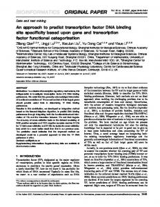
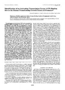
Figures 1 and 2 show a schematic system-like representation of the proposed algorithm. The input parameters to the algorithm are the genome under study G�×� (L is the length of the genome in nucleobases) and the set of binding site sequences belonging to a particular transcription factor represented by the matrix X�×� . The distance metric vector A�×� is assigned to the set of conserved binding sites belonging to the same transcription factor with a length equal to the number of binding sites (N), while B�×(�����) is another distance metric vector assigned to set of sequences in the genome with a length similar to the conserved sequence length (M). The output of the algorithm is a distance vector E�×� that corresponds to the locations of actual binding sites investigated.
Position Frequency Matrix (PFM) Calculation
X ×
PFM
Position Frequency Matrix Correlator
Aଵ× Bଵ×(ିାଵ)
Gଵ×
Fig. 1. TFBS Detection Algorithm (part 1) X × Bଵ×(ିାଵ) �ଵ×
Thresholding T = min{a୧ } i = 1,2, … , N Keep {b୧ ≥ T}
Cଵ×
Choose (c୧ = a୧ )
Dଵ× ow he ith
Verification: Check whether the detected sequence is a conserved sequence or not
Eଵ×ୖ E1 × r
� 2) Fig. 2. TFBS Detection Algorithm (part
2.1
Mathematical Description
The genome under study is given by G�×� = �g� , g � , g , … , g � �,
(1)
where g ∈ �A, G, C, T� is the i� nucleobase in the genome and i = 1, 2, 3, … , L is the genome length in nucleobases. Each set of binding sites belonging to a given transcription factor can be represented as a matrix consisting of N rows and M columns. The number of rows N corresponds to the number of binding sites conserved sequences, and the number of columns M corresponds to the number of nucleobases in each binding site. Hence, each one of the 124 different E. Coli transcription factors (see Table 1) investigated in this paper can be represented as a matrix of size (N×M) denoted as X�×� and is given by Proceedings IWBBIO 2014. Granada 7-9 April, 2014
717
X��
x�� x�� x� x�� x�� x� = ⋮ ⋮ ⋮ x�� x�� x�
… x�� … x��
, ⋱ ⋮ … x��
(2)
where x � ∈ �A, G, C, T�; k = 1, 2, . . . , N; j = 1, 2, … , M. Each row of the matrix X�×� can be represented by a �4 × M� binary matrix (containing only 1's and 0's) where each row corresponds to one of the four nucleobases �A, G, C, T�. For example, if the 5� row of the matrix X�×� is given by the sequence 5’ − CAGGTCTGCA − 3’, then the corresponding binary matrix, denoted as S, will have the form shown in Figure 3. � � � �
� 1 0 1 0 0
� 2 1 0 0 0
3 0 0 1 0
4 0 0 1 0
5 0 0 0 1
� 6 0 1 0 0
7 0 0 0 1
8 0 0 1 0
� 9 0 1 0 0
� 10 1 0 0 0
� �
Fig. 3. The � Matrix of the Fifth Row Sequence in � ۻ×ۼ.
Based on this definition of the S binary matrix, the so-called Position Frequency Matrix, denoted as PFM, can be obtained by averaging the N corresponding S binary matrices that represent the N rows in the X �×� matrix. This makes the Position Frequency Matrix be of a size (4 × M). The (b, l) element in the PFM matrix will then be equal to the frequency of the nucleobase b occurring at position l and hence can be defined as PFM(b, l) = ∑� ��� S�b, l, j�, �
(3)
�
The (4 × M) Position Frequency Matrix can then be rewritten as
r�� r PFM = �� r�� r��
r�� r�� r�� r��
r� r� r� r�
… … … …
r�� r��
. r�� r��
(4)
where r�� = PFM(b, l), b ∈ �A, G, C, T�, and 1 ≤ l ≤ M. The (b, l) elements of the PFM matrix can be alternatively calculated as r�� =
��� �
,
(5)
where l = 1, 2, 3, … , M; N� stands for the number of times the base b ∈ �A, G, C, T� occurs in column l of the matrix X�×� . Therefore, r�� is the probability of the base b occurring at position l. This makes the elements of each row in the PFM matrix add up to one. According to the schematic representation in Figures 1 and 2, the algorithm is able to detect TFBSs in the genome by the following steps:
Proceedings IWBBIO 2014. Granada 7-9 April, 2014
718
Step 1: Position frequency matrix calculation The Position frequency matrix (PFM) can be calculated using equation 3 or alternatively using equations 4 and 5. Step 2: Distance metric vectors calculation After calculating the position frequency matrix (PFM), the next step is to assign each conserved sequence (i.e. each row in X�×� ) a distance metric obtained by first aligning that particular row with the position frequency matrix and then adding up the values in the matrix that correspond to each nucleobase in that row. If any of these values is zero (this means that this particular base does not happen at that position), then we add up the values occurring before this later zero and stop and then move to the next row. Based on this, we get a distance vector (A�×� ) which can be written as A�×� = �a� , a � , a , … , a � �,
(6)
� � � a = ∑��� r���� ,
(7)
B�×(�����) = �b� , b� , b , … , b����� �,
(8)
� � b = ∑� r �� � , ���
(9)
where a is a distance metric associated with the i� row in X�� and is obtained by �
where i = 1, 2, 3, … , N, x � ∈ {A, G, C, T} is the (i, j) element in the X�×� matrix, and M’ is the j� index of the first base in the i� row to map to a zero in the Position Frequency Matrix (PFM). The next step is to compare the whole genome sequence to the set of conserved sequences represented by X�×� . To achieve this, a sliding window of length equal to M (conserved sequence length) is translated all over the genome (G�×� ) one base at a time. This will divide the genome sequence into (L − M + 1) subsequences each of length M. These subsequences are then assigned distance metrics following the same procedure used to get the distance vector A�×� . Hence, this will yield another distance vector, B�×(�����) , which can be written as where b is a distance metric associated with a sequence of length M obtained at the i� nucleobase position of the genome and is defined by �
where i = 1, 2, 3, … , L − M + 1; g ∈ �A, G, C, T� is a base in the genome being considered. r�� � is the j� element in the PFM matrix that corresponds to the i� base in the genome (g ), and M’ is the j� index of the first base in the i� subsequence in the genome to map to a zero in the Position Frequency Matrix. Step 3: Thresholding of the distance vector B�×������� . At this point, the weighting vector B�×(�����) contains all the possible weights corresponding to all possible conserved sequences in the genome sequence. The higher the weight value of a given sequence, the higher is the probability of that particular
Proceedings IWBBIO 2014. Granada 7-9 April, 2014
719
sequence to be a real conserved sequence. To eliminate those subsequences in the genome with low weights, a threshold T is calculated as the minimum weight in the distance vector A�×� vector obtained in step 2. All the weights less than T are discarded. The resulting weighting vector after Thresholding (C�× ) is defined as
C�×� = �c = b� ; b� ≥ T�,
(6)
T = min�a �,
(7)
D�� = �d = c� ; c� = a � �,
(8)
where i = 1, 2, 3, … , K; j = 1, 2, 3, … , L − M + 1. The threshold T is defined as
where i = 1, 2, 3, … , N. Now, the vector C�×� contains all the possible weights greater than or equal to the threshold T. In other words, the vector C�×� gives the locations of the subsequences in the genome that are of either exact or of high similarity to the given set of binding sites. As we want to only keep the locations of the subsequences in the genome that are of total similarity to the set of conserved sequences, all the values in C�×� that are different from the set of weights in the A�×� vector are discarded. The resulting weighting vector can be written as
where i = 1, 2, 3, … , P; j = 1, 2, 3, … , K and P ≤ K.
Step 4: TFBS Identification. Although at this point of the algorithm we have drastically decreased the number of possible conserved sequences, we still have too many possible sequences belonging to the genome that are not real conserved sequences (false positives). The vector D�� contains all the possible weights that are exactly the same as the weights of the original conserved sequences. Some of these weights are false positive, i.e. they do not correspond to an actual conserved sequence. To filter these false positives out, each one of the detected sequences is compared to the original conserved sequences and only the verified ones are kept. The resulting distance vector E�� is evaluated as
E�� = �e = d� ; S�d� � = X(d� ), �,
(9)
where i = 1, 2, 3, … , R; j = 1, 2, 3, … , P; S�d� � is the sequence of length M in the genome corresponding to the j� weight in the D�×� vector. X(d� ) is the conserved sequence in X�×� having the same weight d� since if these two sequences are the same, they have to have the same weight value.
3
Analysis and Simulation Results
In order to be able to handle the conserved sequences of all transcription factors investigated in this paper, a database (a cell array in MATLAB) is built where each TF is assigned a number. Since Escherichia coli (E. coli) is a well-studied organism with
Proceedings IWBBIO 2014. Granada 7-9 April, 2014
720
several highly accurately annotated genome sequences, it is used here as a test case. As such, a database of E. coli transcription factor binding sequences is produced. Table 1 shows 124 different E. coli transcription factors obtained from Regulon database [17], and Ecogene database [18]. Sequences were collated, redundancies were eliminated, and validated by identifying them in the E. coli genome in Ecogene. Table 1. E. Coli Transcription Factors. FN 1 2 3 4 5 6 7 8 9 10 11 12 13 14 15 16 17 18 19 20 21 22 23 24 25 26 27 28 29 30 31
TF AcrR Ada AgaR AlaS AllR AraC ArcA ArcR ArgR AtoC BaeR BetI BirA CRP CaiF Cbl ChbR CpxR CsgD CspA CueR CusR CynR CysB CytR DcuR DeoR DgsA DnaA EnvY EvgA
FN 32 33 34 35 36 37 38 39 40 41 42 43 44 45 46 47 48 49 50 51 52 53 54 55 56 57 58 59 60 61 62
TF ExuR FNR FabR FadR FhlA Fis FlhDC FruR Fur GadE GalR GcvA GlcC GlpR GntR H-NS HU HcaR HipB HyfR IHF IclR IdnR IscR KdgR KdpE LacI LexA LldR LrhA Lrp
FN 63 64 65 66 67 68 69 70 71 72 73 74 75 76 77 78 79 80 81 82 83 84 85 86 87 88 89 90 91 92 93
TF MalI MalT MarA MarR MelR MetJ MetR MhpR MngR ModE MprA MtlR Nac NagC NanR NarL NarP NhaR NikR NorR NrdR NsrR NtrC OmpR OxyR PaaX PdhR PepA PhoB PhoP PrpR
FN 94 95 96 97 98 99 100 101 102 103 104 105 106 107 108 109 110 111 112 113 114 115 116 117 118 119 120 121 122 123 124
TF PspF PurR QseB RbsR RcsAB RhaR RhaS Rob RstA RutR SdiA SgrR SlyA SoxR SoxS TdcA TdcR TorR TreR TrpR TyrR UhpA UidR UlaR UxuR XapR XylR YiaJ ZntR ZraR Zur
The proposed algorithm for TFBS detection is applied to two Escherichia coli bacterial genomes namely: MG1655 and O157:H7 E. coli strains (both forward and reverse strands were investigated). Figures 4-7 show the simulation results obtained when the algorithm was applied to MG1655 positive strand, MG1655 negative strand, O157:H7 positive strand and O157:H7 negative strand, respectively. The red color in these figures corresponds to the set of TFBSs detected in the non-coding regions, the blue color to the ones detected in the coding regions, and the green color to the ones overlapping between non-coding and coding regions. The y-axis in Figures 4-7 represents the transcription factor number with some offset values introduced to distinguish the three set of detected TFBSs as located in the non-coding regions (marked in red or the ones below the 124 horizontal line) or in the coding regions (marked in green or above the 248 horizontal line) or overlapping in
Proceedings IWBBIO 2014. Granada 7-9 April, 2014
721
between (marked in blue or between 124 and 248 horizontal lines). The offset values are 124 and 248. In other words, any horizontal line below 124 will pass through all the TFBSs related to the transcription factor indexed by the y-axis value. If this horizontal line is between 124 and 248 (i.e. the middle region) a value of 124 should be subtracted from the y-axis value to know what transcription factor is being referred to. Finally, if the horizontal line is above 248 then a value of 248 should be subtracted. In this way, Figures 4-7 not only classify the detected TFBSs into three different sets but also tell which transcription factor is being referred to at each level. According to the simulation results shown in Figures 4-7, Table 2 gives some statistical information of the detected TFBSs in terms of percentages. As can be observed, most of the detected TFBSs are located in the non-coding regions which is biologically relevant and agrees with theory [9] as the transcription factors which bind to the detected sites regulate the transcription of the adjacent genes located ahead. 500
Noncoding Region Coding Region Overlapping Region
Transcription Factor Number
450
400
350
300
250
200
150
100
50
0 0
0.5
1
1.5
2
2.5
3
3.5
4
Base Position
4.5 x 10
6
Fig. 4. TFBS detection using MG1655 positive strand 500
Taranscription Factor Number
450
Noncoding Region Coding Region Overlapping Region
400
350
300
250
200
150
100
50
0 0
0.5
1
1.5
2
2.5
Base Position
3
3.5
4
4.5 x 10
6
Fig. 5. TFBS detection using MG1655 negative strand
Proceedings IWBBIO 2014. Granada 7-9 April, 2014
722
500
Noncoding Region Coding Region Overlapping Region
Transcription Factor Number
450
400
350
300
250
200
150
100
50
0 0
0.5
1
1.5
2
2.5
3
3.5
4
4.5
5
Base Position
x 10
6
Fig. 6. TFBS detection using O157:H7 positive strand 500
Noncoding Region Coding Region Overlapping Region
Transcription Factor Number
450
400
350
300
250
200
150
100
50
0 0
0.5
1
1.5
2
2.5
3
3.5
Base Position
4
4.5
5 x 10
6
Fig. 7. TFBS detection using �157: �7 negative strand Table 2. TFBSs detected in MG1655 and O175:H7 E. coli strains E. coli Strain Strand Orientation Total number of TFBSs % of TFBSs in non-coding regions % of TFBSs in the coding regions % of TFBSs overlapping in between
3.1
MG1655 Positive Negative Strand Strand 956 1000 85.46 85.90 6.49 6.20 8.05 7.90
O157:H7 Positive Negative Strand Strand 642 616 86.15 85.23 6.85 5.84 7.00 8.93
Discovery of New Motif Sequences
In the gene expression process, it is very common that a single transcription factor binds not to an exact motif sequence but rather to a consensus motif. This fact is due to some bases belonging to the motif sequence are not as important as others when a transcription factor binds in the binding site. To consider this in the developed algorithm, the search for possible TFBSs was modified such that if the subsequence being tested is more that 80% (this number can be modified as required) similar to the original corresponding set of TFBSs, then it can be considered as a possible TFBS. For example, applying the algorithm to MG16655 E. coli genome (forward strand) to locate subsequences of similitude greater than or equal to 80% of their original corresponding sets of TFBSs, yields six other possible sequences. Table 3 gives a detailed
Proceedings IWBBIO 2014. Granada 7-9 April, 2014
723
description of these six sequences with their corresponding location in the genome, the transcription factor they belong to, the number of matching bases and the percentage of similitude of these sequences with their original corresponding transcription factor binding sites. Table 4 show similar simulation results but with the percentage of similitude being set to 70%. By so doing, thirty two subsequences result. Therefore, this algorithm does not only provide locations of the sets of verified conserved sequences but also locations of all subsequences of the genome that are partially similar as well (with a predefined percentage of similitude as required). This freedom in introducing this percentage of similitude between the target sequences to be located and the original transcription factor binding sites allows for more flexibility in detection. Table 3. Possible motif sequences based on greater than 80% similitude to their original sets of TF conserved sequences #
Possible ���
Base Position
TF #
TF
# of Matches
Similarity Percentage
1 2 3 4 5 6
'AGGCCUACGUUAAUUCUGCAAUAUAUUGAAUCU' 'AGGCCUACGUUAUUUCAGCAAUAUAUUGAAUUU' 'AGGCCUACGUGAACUCUGCAAUAUAUUGAAUUU' 'AGGCCUACAUGAUUUCUGCAAUAUAUUGAAUUU' 'UGGUAUAACAGGUAUAAAGGUAUACA' 'UUAUACCUGUUAUACCAGAUCAAUUA'
5593 4.3021e+005 8.3153e+005 3.7386e+006 4.5012e+006 3.3713e+006
52 52 52 52 77 77
FNR FNR FNR FNR DcuR DcuR
29 28 29 28 24 24
87.879 84.848 87.879 84.848 92.308 92.308
Table 4. Possible motif sequences based on greater than 70% similitude to their original sets of binding sites #
�
���� ����
1 2 3 4 5 6 7 8 9 10 11 12 13 14 15 16 17 18 19 20 21 22 23 24 25 26 27 28
′AGGCCUACGUUAAUUCUGCAAUAUAUUGAAUCU′ ′AGGCCUACGUUAUUUCAGCAAUAUAUUGAAUUU′ ′AGGCCUACAUGAUCUCUGCAAUAUAUUGAGUUU′ ′AGGCCUACAUUUUCUCCGCAAUAUAUUGAAUUU′ ′AGGCCUACGUGAACUCUGCAAUAUAUUGAAUUU′ ′AGGCCUACAUGAUUUCUGCAAUAUAUUGAAUUU′ ′AGGCCAACGGUAGAAUUGUAAUCUAUUGAAUUU′ ′UUAAUUAAAAUGUUACGUGUUUAAUGU′ ′UAUUUAAAUUUUUUGUGCUUUUGUUUU′ ′ACAUUAAAAAUGAAACUUAUUAAAUUG′ ′UUGAUUAAAAAGGUAAAUAUUUAAAAU′ ′UAUUUUUUGUUUUUAUUUUUUAAAGGA′ ′UUAAUAAAAAUGAUGAAUGAUUUAGAC′ ′CUGUACAUAUCAUAGACUAAACGGAUAC′ ′UGGUAUAACAGGUAUAAAGGUAUACA′ ′UUAUACCUGUUAUACCAGAUCAAUUA′ ′CAUAGAGGUUUAAUCCUUAUUCAGAGU′ ′GUCACUAUACAACGGACGGGGGAAGGA′ ′AAUUGCAUUUAAAAAAUAUGUUCUGUG′ ′UGAUAUCACUAUAGAUAUUGAUCAUUA′ ′UAUUACAAUGUAAUCAUUAAUUGCUAA′ ′UGAACUCAGUAAGAGCAGUGAUAAUCA′ ′CUUAAUGAAGUACUCAAUAGAUUUGUU′ ′AUUGCUAAUGAAAAACAUCAAUCCAAC′ ′UUAGGUAUUGAUAACAAUCAAUAGUAC′ ′GUCAUGAUGGCGCAUUAUUUUGUGGUG′ ′UUACCGCUGGUGCCGCAGGUCAGUUUC′ ′UUACCCAUGAAGCGGUAGGUAAAUGUG′
�� � � ��� � 5593 4.3021% + 005 7.0708% + 005 8.1483% + 005 8.3153% + 005 3.7386% + 006 4.0476% + 006 5.2862% + 005 1.2187% + 006 1.5962% + 006 2.9025% + 006 3.4946% + 006 3.5807% + 006 1.7994% + 006 4.5012% + 006 3.3713% + 006 2.4967% + 006 4.363% + 006 3.8409% + 005 1.3899% + 006 1.9563% + 006 2.1632% + 006 2.4831% + 006 4.2313% + 006 4.5015% + 006 5.3802% + 005 1.3878% + 006 1.8717% + 006
Proceedings IWBBIO 2014. Granada 7-9 April, 2014
�� #
��
52 52 52 52 52 52 52 53 53 53 53 53 53 68 77 77 78 78 78 78 78 78 78 78 78 78 78 78
"#$ "#$ "#$ "#$ "#$ "#$ "#$ "&'( "&'( "&'( "&'( "&'( "&'( )%*+ ,-.( ,-.( ,-/0 ,-/0 ,-/0 ,-/0 ,-/0 ,-/0 ,-/0 ,-/0 ,-/0 ,-/0 ,-/0 ,-/0
# � ������ 29 28 26 25 29 28 24 19 19 19 19 20 19 20 24 24 19 19 19 19 19 19 19 19 19 19 19 20
��������� ��������!� 87.879 84.848 78.788 75.758 87.879 84.848 72.727 70.37 70.37 70.37 70.37 74.074 70.37 71.429 92.308 92.308 70.37 70.37 70.37 70.37 70.37 70.37 70.37 70.37 70.37 70.37 70.37 74.074
724
29 30 31 32
′GGUAUCAAACUUCUCUUUAAACAGAUA′ ′CUAUUGCUUGUGCGGUAUUUGCCAAAA′ ′UUUAAUAAAAAAAAGAUUAAGGGAUGA′ ′AUACUAUCACUACCCUUUUUUUACACA′
4.2953% + 006 1.8083% + 006 5.834% + 005 3.6487% + 006
78 78 78 79
,-/0 ,-/0 ,-/0 ,-/1
19 20 19 19
70.37 74.074 70.37 70.37
Based on the high similitude of the sequences detected in Tables 3 and 4 of their original corresponding sets of TFBSs, they can be considered as possible motif sequences. These sequences can be tested to see if they appear in other E. coli genomes. If yes, this will increase the chance that these sequences are potential TFBSs. Hence, they will need to be subjected to biological experiments to verify their significance. This type of analysis was applied to MG1655 and O157:H7 E. coli strains.
4
Conclusion
In this paper, a novel algorithm for transcription factor binding site (TFBS) detection is proposed. The algorithm is based on a position frequency matrix concept to design distance metrics that quantify the similitude between the set of conserved sequences and the entire DNA sequence under study. This algorithm does not use any type of mapping for the nucleobases and hence independent of mapping. The developed algorithm is applied to two different E. coli bacterial genomes (namely: MG1655 and O157:H7). Simulation results show that around 85% of the detected TFBSs are located in the non-coding region, 6.5% are located in the coding regions, and only 8.5% are overlapped between coding and non-coding regions. This shows that the proposed algorithm is not only able to efficiently identify and accurately locate the known TFBSs in their exact positions in the entire genome sequence, but also can be utilized in the discovery of new motif sequences based on their similitude to the known TFBSs with a predefined percentage of similitude as required. Having analyzed only two E. coli genomes, six possible motif sequences were detected (as shown in Table 3) based on an 80% similitude constraint, while thirty two possible motif sequences were detected (as shown in Table 3) based on a 70% similarity constraint. Therefore, if this method of motif finding is applied to more other genomes as done in a previous work [1], other potential motif sequences can be identified. Hence, the previous analysis of using the position frequency matrix based algorithm to detect and identify new motif sequences can efficiently yield other potential motif candidates that are recommended for further analysis. Future work can utilize the results obtained in this paper to help distinguish coding and non-coding regions. In other words, the developed analyses here can help in the gene identification problem. REFERENCES 1. Mohammad Al Bataineh, Lun Huang, and G. Atkin, "TFBS detection algorithm using distance metrics based on center of mass and polyphase mapping," in 2012 7th International Symposium on Health Informatics and Bioinformatics (HIBIT), Cappadocia, Turkey, 2012, pp. 37-40.
Proceedings IWBBIO 2014. Granada 7-9 April, 2014
725
2. I. Erill and M. C. O'Neill, "A reexamination of information theory-based methods for DNA-binding site identification," BMC Bioinformatics, vol. 10, p. 57, 2009. 3. Sailu Yellaboina, Jayashree Seshadri, M. Senthil Kumar, and A. Ranjan, "PredictRegulon: a web server for the prediction of the regulatory protein binding sites and operons in prokaryote genomes," Nucleic Acids Research 32 (Web-Server-Issue), pp. 318-320, 2004. 4. Richard Münch, Karsten Hiller, Andreas Grote, Maurice Scheer, Johannes Klein, M. Schobert, and D. Jahn, "Virtual Footprint and PRODORIC: an integrative framework for regulon prediction in prokaryotes," Bioinformatics, vol. 21, pp. 4187-4189, 2005. 5. G. D. Stormo, "DNA binding sites: representation and discovery," Bioinformatics, vol. 16, pp. 16-23, Jan 2000. 6. D. Bisant and J. Maizel, "Identification of ribosome binding sites in Escherichia coli using neural network models," Nucleic Acids Res, vol. 23, pp. 1632-9, May 11 1995. 7. M. C. O'Neill, "Training back-propagation neural networks to define and detect DNAbinding sites," Nucleic Acids Res, vol. 19, pp. 313-8, Jan 25 1991. 8. M. K. Das and H.-K. Dai, "A survey of DNA motif finding algorithms," BMC Bioinformatics, 2007. 9. C. Jia, M. B. Carson, and J. Yu, "A Fast Weak Motif-Finding Algorithm Based on Community Detection in Graphs," BMC Bioinformatics, vol. 14, 2013. 10. T. L. Bailey, "Discovering sequence motifs," Methods Mol Biol, vol. 452, pp. 231-51, 2008. 11. T. L. Bailey and C. Elkan, "The value of prior knowledge in discovering motifs with MEME," in Proceedings of the Third International Conference on Intelligent Systems for Molecular Biology, Menlo Park, CA, 1995, pp. 21–29. 12. G. Z. Hertz and G. D. Stormo, "Identifying DNA and protein patterns with statistically significant alignments of multiple sequences," Bioinformatics, vol. 15, pp. 563–577, 1999. 13. C. E. Lawrence, S. F. Altschul, M. S. Boguski, J. S. Liu, A. F. Neuwald, and J. C. Wootton, "Detecting subtle sequence signals: a Gibbs sampling strategy for multiple alignment," Science, vol. 262, pp. 208-14, Oct 8 1993. 14. R. Siddharthan, E. D. Siggia, and E. van Nimwegen, "PhyloGibbs: a Gibbs sampling motif finder that incorporates phylogeny," PLoS Comput Biol, vol. 1, p. e67, Dec 2005. 15. S. RA and S. DJ, "Inclusion of Neighboring Base Interdependencies Substantially Improves Genome-Wide Prokaryotic Transcription Factor Binding Site Prediction," Nucleic Acids Research, vol. 38, 2010. 16. E. L, J. VX, F. PJ, and J. SJ, "Locating Mammalian Transcription Factor Binding Sites: A Survey of Computational and Experimental Techniques," Genome Res, vol. 16, pp. 14551464, 2006. 17. E. van Nimwegen, "Scaling laws in the functional content of genomes," Trends Genet, vol. 19, pp. 479-84, Sep 2003. 18. K. E. Rudd, "EcoGene: a genome sequence database for Escherichia coli K-12," Nucleic Acids Res, vol. 28, pp. 60-4, Jan 1 2000.
Proceedings IWBBIO 2014. Granada 7-9 April, 2014
726