Tree Induction vs. Logistic Regression: A Learning ... - SSRN papers

Tree Induction vs. Logistic Regression: A Learning{Curve Analysis Claudia Perlich, Foster Provost, and Jerey S. Simono Leonard N. Stern School of Business New York University 44 West 4th Street New York, NY 10012 December 13, 2001

Abstract Tree induction and logistic regression are two standard, o{the{shelf methods for building models for classication. We present a large{scale experimental comparison of logistic regression and tree induction, assessing classication accuracy and the quality of rankings based on class-membership probabilities. We use a learning{curve analysis to examine the relationship of these measures to the size of the training set. The results of the study show several remarkable things. (1) Contrary to prior observations, logistic regression does not generally outperform tree induction. (2) More specically, and not surprisingly, logistic regression is better for smaller training sets and tree induction for larger data sets. Importantly, this often holds for training sets drawn from the same domain (i.e., the learning curves cross), so conclusions about induction-algorithm superiority on a given domain must be based on an analysis of the learning curves. (3) Contrary to conventional wisdom, tree induction is eective at producing probability{based rankings, although apparently comparatively less so for a given training{set size than at making classications. Finally, (4) the domains on which tree induction and logistic regression are ultimately preferable can be characterized surprisingly well by a simple measure of signal-to-noise ratio.

1 Introduction In this paper we show that combining massive experimental comparison of learning algorithms with the examination of learning curves can lead to new insights into the relative performance of learning algorithms. We also show that by 1

comparing algorithm performance on larger data sets we see behavioral characteristics that would be overlooked when comparing algorithms on smaller data sets (such as most in the UCI repository). More specically, we examine several dozen large, two-class data sets, ranging from roughly one thousand examples to two million examples. We assess performance based on classication accuracy, and based on the area under the ROC curve (which measures the ability of a classication model to score cases by likelihood of class membership). We compare two basic algorithm types (logistic regression and tree induction), including variants that attempt to address the algorithms' shortcomings. We selected these particular algorithms for several reasons. First, they are popular (tree induction with machine learning researchers, logistic regression with statisticians and econometricians). Second, they all can produce class{ probability estimates. Third, they typically are competitive o the shelf (i.e., they usually perform relatively well with no parameter tuning).1 O{the{shelf methods are especially useful for non{experts, and also can be used reliably as learning components in larger systems. For example, a Bayesian network learner has a dierent probability learning subtask at each node manual parameter tuning for each is infeasible, so automatic (push{button) techniques typically are used (Friedman and Goldszmidt, 1996). Finally, we selected these methods because of a dierence of opinion that seems to be manifest (traditionally) between the statistics community and the machine learning community. Although it is changing in both communities, machine learning researchers and practitioners have preferred nonparametric methods such as tree induction, while statisticians have preferred parametric methods such as logistic regression. Note, interestingly, that until recently few machine learning research papers considered logistic regression in comparative studies. C4.5 (Quinlan, 1993) is the typical benchmark learning algorithm. However, the study by Lim, Loh, and Shih (2000) shows that on UCI data sets, logistic regression beats C4.5 in terms of classication accuracy. We investigate this phenomenon carefully, and our results suggest that this is due, at least in part, to the small size of the UCI data sets. When applied to larger data sets, learning methods based on C4.5 usually are more accurate. Our investigation has three related goals. 1. To compare the broad classes of tree induction and logistic regression. The literature contains various anecdotal and small{scale comparisons of these two approaches, but no systematic investigation that includes several very large data sets. 2. To compare, on the same footing and on large data sets, dierent variants of these two families, including Laplace \smoothing" of probability estimation trees, model selection applied to logistic regression, biased (\ridge")

1 In fact, logistic regression has been shown to be extremely competitivewith other learning methods (Lim, Loh, and Shih, 2000), as we discuss in detail.

2

logistic regression, and bagging applied to both methods. 3. To compare the learning curves of the dierent types of algorithm, in order to explore the relationship between training{set size and induction algorithm. Learning curves allow us to see patterns (when they exist) that depend on training{set size and that are common across dierent data sets. From the ultimate learning-curve analysis we can draw several conclusions.









Logistic regression performs better, generally and relatively speaking, for smaller data sets and tree induction performs better for larger data sets. This relationship holds (often) even for data sets drawn from the same domain|that is, the learning curves cross. Therefore, drawing conclusions about one algorithm being better than another for a particular domain is questionable without an examination of the learning curves. Tree{based probability estimation models often outperform logistic regression for producing probability{based rankings (for which logistic regression is the statistical method of choice), especially for larger data sets. The domains on which each type of algorithm performs better can be characterized remarkably consistently by a measure of signal{to{noise ratio.

The rest of the paper is structured as follows. First we give some background information for context. Then we describe the algorithms and their variants that we will consider. We then describe the basic experimental setup, including the data sets that we will use, the evaluation metrics, the method of learning curve analysis, and the particular implementations of the learning algorithms. Next we present the results of two sets of experiments, done individually on the two classes of algorithms, to assess the sensitivity of performance to the algorithm variants (and therefore the necessity of these variants). We use this analysis to select a subset of the methods for the nal analysis. We then present the nal analysis, comparing across the algorithm families, across dierent data sets, and across dierent training{set sizes. The upshot of the analysis is that there seem to be clear conditions under which each family is preferable. Tree induction is preferable for larger training{ set sizes with lower noise levels. Logistic regression is preferable for smaller training{set sizes and for higher noise levels. We were surprised that the relationship is so clear, given that we do not know of its having been reported previously in the literature. However, it ts well with our basic knowledge (and assumptions) about tree induction and logistic regression. We discuss this and further implications at the close of the paper.

3

2 Background The machine learning literature contains many studies comparing the performance of dierent inductive algorithms, or algorithm variants, on various benchmark data sets. The purpose of these studies typically is (1) to investigate which algorithms are better generally, or (2) to demonstrate that a particular modication to an algorithm improves its performance. For example, Lim, Loh, and Shih (2000) present a comprehensive study of this sort, showing the dierences in accuracy, running time, and model complexity of several dozen algorithms on several dozen data sets. Papers such as this seldom consider carefully the size of the data sets to which the algorithms are being applied. Does the relative performance of the dierent learning methods depend on the size of the data set? As we describe in detail below, learning curves compare the generalization performance (e.g., classication accuracy) obtained by an induction algorithm as a function of training-set size. More than a decade ago in machine learning research, the examination of learning curves was commonplace (see, for example, Kibler and Langley, 1988), but usually on single data sets (notable exceptions being the study by Shavlik, Mooney, and Towell (1991) and the work of Catlett (1991)). Now learning curves are presented only rarely in comparisons of learning algorithms.2 The few cases that exist draw conicting conclusions, with respect to our goals. Domingos and Pazzani (1997) compare classication{accuracy learning curves of naive Bayes and the C4.5rules rule learner (Quinlan, 1993). On synthetic data, they show that naive Bayes performs better for smaller training sets and C4.5rules performs better for larger training sets (the learning curves cross). They discuss that this can be explained by considering the different bias/variance proles of the algorithms for classication (zero/one loss). Roughly speaking,3 variance plays a more critical role than estimation bias when considering classication accuracy. For smaller data sets, naive Bayes has a substantial advantage over tree or rule induction in terms of variance. They show that this is the case even when (by their construction) the rule learning algorithm has no bias. As expected, as larger training sets reduce variance, C4.5rules approaches perfect classication. Brain and Webb (1999) perform a similar bias/variance analysis of C4.5 and naive Bayes. They do not examine whether the curves cross, but do show on four UCI data sets that variance is reduced consistently with more data, but bias is not. These results do not directly examine logistic regression, but the bias/variance arguments do apply: logistic regression, a linear model, should have higher bias but lower variance than tree induction. Therefore, one would expect that their learning curves might cross. However, the results of Domingos and Pazzani were generated from synthetic data where the rule learner had no bias. Would we see such behavior on realworld domains? Kohavi (1996) shows classication{accuracy learning curves of Learning curves also are found in the statistical literature (Flury and Schmid, 1994) and in the neural network literature (Cortes et al., 1994). 3 Please see the detailed treatment by Friedman (1997). 2

4

tree induction (using C4.5) and of naive Bayes for nine UCI data sets. With only one exception, either naive Bayes or tree induction dominates (i.e., the performance of one or the other is superior consistently for all training{set sizes). Furthermore, by examining the curves, Kohavi concludes that \In most cases, it is clear that even with much more data, the learning curves will not cross" (pp. 203{204). We are aware of only one learning-curve analysis that compares logistic regression and tree induction. Harris{Jones and Haines (1997) compare them on two business data sets, one real and one synthetic. For these data the learning curves cross, suggesting (as they observe) that logistic regression is preferable for smaller data sets and tree induction for larger data sets. Our results generally support this conclusion.

3 Algorithms for the analysis of binary data We now describe tree induction and logistic regression in more detail, including several variants examined in this paper. The particular implementations used are described in detail in Section 4.4.

3.1 Tree induction for classication and probability estimation

The terms \decision tree" and \classication tree" are used interchangeably in the literature. We will use \classication tree" here, in order that we can distinguish between trees intended to produce classications, and those intended to produce estimations of class probability (\probability estimation trees"). When we are talking about the building of these trees, which for our purposes is essentially the same for classication and probability estimation, we will simply say \tree induction." We would like for this paper to be comprehensible to both machine learning researchers and to statisticians, so we will describe both tree induction and logistic regression in detail. A reader knowledgeable in either area can safely skip the \basic" material.

3.1.1 Basic tree induction

Classication{tree learning algorithms are greedy, \recursive partitioning" procedures. They begin by searching for the single predictor variable x
1 that best partitions the training data (as determined by some measure). This rst selected predictor, x
1 , is the root of the learned classication tree. Once x
1 is selected, the training data are partitioned into subsets satisfying the values of the variable. Therefore, if x
1 is a binary variable, the training data will be partitioned into two subsets. The classication{tree learning algorithm proceeds recursively, applying the same procedure to each subset of the partition. The result is a tree of predictor 5

variables, each splitting the data further. Dierent algorithms use dierent criteria to evaluate the quality of the splits produced by various predictors. Usually, the splits are evaluated by some measure of the \purity" of the resultant subsets, in terms of the outcomes. For example, consider the case of binary predictors and binary outcome: a maximally impure split would result in two subsets, each with the same ratio of the contained examples having y = 0 and having y = 1. On the other hand, a pure split would result in two subsets, one having all y = 0 examples and the other having all y = 1 examples. Dierent classication{tree learning algorithms also use dierent criteria for stopping growth. The most straightforward method is to stop when the subsets are pure. On noisy, real{world data, this often leads to very large trees, so often other stopping criteria are included (e.g., stop if one child subset would have fewer than a predetermined number of examples, or stop if a statistical hypothesis test cannot conclude that there is a signicant dierence between the subsets and the parent set). The data subsets produced by the nal splits are called the leaves of the classication tree. More accurately, the leaves are dened intensionally by the conjunction of conditions along the path from the root to the leaf. For example, if binary predictors dening the nodes of the tree are numbered by a (depth{rst) pre{order traversal, and predictor values are ordered numerically, the rst leaf would be dened by the logical formula: (x
1 = 0) ^ (x
2 = 0) ^    ^ (x
d = 0), where d is the depth of the tree along this path. An alternative method for controlling tree size is to prune the classication tree. Pruning involves starting at the leaves, and working upward toward the root (by convention, classication trees grow downward), repeatedly asking the question: should the subtree rooted at this node be replaced by a leaf? As might be expected, there is a wide variety of pruning algorithms. One of the most common approaches is \reduced{error pruning," which replaces a subtree with a leaf if the subtree does not improve accuracy (Quinlan, 1987). Assessments of improvement are done on the training set, or on a subset of the training data held out specially for this purpose. Classications also are produced by the resultant classication tree in a recursive manner. A new example is compared to x
1 , at the root of the tree depending on the value of this predictor in the example, it is passed to the subtree rooted at the corresponding node. This procedure recurses until the example is passed to a leaf node. At this point a decision must be made as to the classication to assign to the example. Typically, the example is predicted to belong to the most prevalent class in the subset of the training data dened by the leaf. It is useful to note that the logical formulae dened by the leaves of the tree form a mutually exclusive partition of the example space. Thus, the classication procedure also can be considered as the determination of which leaf formula applies to the new example (and the subsequent assignment of the appropriate class label).

6

3.1.2 Laplace{corrected probability estimation trees (PETs)

A straightforward method of producing an estimate of the probability of class membership from a classication tree is to use the frequency of the class at the corresponding leaf, resulting in a probability estimation tree (PET). For example, if the leaf matching a new example contains p positive examples and n negative examples, then the frequency{based estimate would predict the probability of membership in the positive class to be p+p n . It has been noted (see, for example, the discussion by Provost and Domingos, 2000) that frequency{based estimates of class{membership probability, computed from classication{tree leaves, are not always accurate. One reason for this is that the tree{growing algorithm searches for ever{more pure leaves. This search process tends to produce overly extreme probability estimates. This is especially the case for leaves covering few training examples. To produce better class{probability estimates, \smoothing" can be used at the leaves. A detailed investigation of smoothing methods is beyond the scope of this paper. However, the use of \Laplace" smoothing has been shown to be particularly eective, and is quite simple. Specically, consider the following potential problem with the frequency{ based method of probability estimation. What if a leaf covers only ve training instances, all of which are of the positive class? Is it reasonable to use a probability estimator that gives an estimate of 1.0 (5/5) that subsequent instances matching the leaf's conditions also will be positive? Perhaps ve instances is not enough evidence for such a strong statement? The so{called Laplace estimate (or Laplace correction, or Laplace smoothing) works as follows (described for the general case of C classes). Assume there are p examples of the class in question at a leaf, N total examples, and C total classes. The frequency{based estimate presented above calculates the estimated probability as Np . The Laplace estimate calculates the estimated probability as p+1 N +C . Thus, while the frequency estimate yields a probability of 1.0 from the p = 5
N = 5 leaf, for a two{class problem the Laplace estimate yields a prob5+1 = 0:86. The Laplace correction can be viewed as a form of ability of 5+2 Bayesian estimation of the expected parameters of a multinomial distribution using a Dirichlet prior (Buntine, 1991). It eectively incorporates a prior probability of C1 for each class (note that with zero examples the probability of each class is C1 ). This may or may not be desirable for a specic problem however, practitioners have found the Laplace correction worthwhile. To our knowledge, the Laplace correction was introduced in machine learning by Niblett (1987). Clark and Boswell (1991) incorporated it into the CN2 rule learner, and its use is now widespread. The Laplace correction (and variants) has been used for tree learning by some researchers and practitioners (Pazzani et al., 1994 Bradford et al., 1998 Provost, Fawcett, and Kohavi, 1998 Bauer and Kohavi, 1999 Danyluk and Provost, 2001), but others still use frequency{based estimates.

7

3.1.3 PETs and pruning

If we're going to compare tree induction to logistic regression using their probability estimates, we also have to consider the eect of pruning. In particular, the pruning stage typically tries to nd a small, high{accuracy tree. The problem for PETs is that pruning removes both of two types of distinctions made by the classication tree: (i) false distinctions|those that were found simply because of \overtting" idiosyncrasies of the training data set, where removal is desirable, and (ii) distinctions that indeed generalize (e.g., entropy in fact is reduced), and in fact will improve class probability estimation, but do not improve accuracy, where removal is undesirable. This is discussed in detail by Provost and Domingos (2000), who also show that pruning indeed can substantially reduce the quality of the probability estimates. When inducing PETs, we therefore will consider unpruned trees with Laplace smoothing.

3.1.4 Bagging

It is well known that trees suer from high variability, in the sense that small changes in the data can lead to large changes in the tree|and, potentially, corresponding changes in probability estimates (and therefore in class labels). Bagging (bootstrap aggregating) was introduced by Breiman (1996) to address this problem, and has been shown to work well often in practice (Bauer and Kohavi, 1999). Bagging produces an ensemble classier by selecting B dierent training data sets using bootstrap sampling (Efron and Tibshirani, 1993) (sampling N data points with replacement from a set of N total data points). Models are induced from each of the B training sets. For classication, the prediction is taken to be the majority (plurality) vote of the B models. We use a variant of bagging that applies to class probability estimation as well as classication. Specically, to produce an estimated probability of class membership, the probability estimates from the B models are averaged. For classication, the class with the highest estimated membership probability is chosen.

3.2 Logistic regression

3.2.1 Basic multiple logistic regression

The standard statistical approach to modeling binary data is logistic regression. Logistic regression is a member of the class of generalized linear models, a broad set of models designed to generalize the usual linear model to target variables of many dierent types (McCullagh and Nelder, 1989 Hosmer and Lemeshow, 2000). The usual (least squares) linear model hypothesizes that an observed target value yi is normally distributed, with mean E (yi ) = 0 + 1 x1i +    + p xpi (1) and variance 2 . That is, the model species an appropriate distribution for yi (in this case, the normal) and the way that the predictors relate to the mean of 8

yi (in this case, the linear relationship (1)). Generalized linear models generalize this by separating model specication into three parts, which allows the data analyst the exibility to change the specication to be appropriate for the data at hand: the distribution of the ith example of the target variable yi (the random component), the way that the predicting variables combine to relate to the level of yi (the systematic component), and the connection between the random and systematic components (the link function). The random component requires that the distribution of yi come from the exponential family, with density function f (y 
) = expfy ; b()]=a() + c(y
)g
for specied functions a(), b(), and c(). The parameter  is called the canonical parameter, and is related to the level of y, while  is a dispersion (variance) parameter. For the standard linear model, f is the normal (Gaussian) density with  =  and  = 2. The systematic component species that the predictor variables relate to the level of y as a linear combination the predictor values, i = 0 + 1 x1i +    + p xpi (a linear predictor). The link function then relates to the mean of y, , being the function g such that g() = (for the standard linear model =  = ). To train the model, the parameters of the generalized linear model are estimated using the method of maximum likelihood in particular, the parameters are chosen to maximize the log{likelihood function n
X yi i ; b(i ) + c(y
) : L= i ai () i=1 A particularly simple form of the generalized linear model, with desirable theoretical properties, occurs when the link function satises g() = . This link is called the canonical link. Consider now the binary (0/1) target variable y of interest here. The appropriate random component for a target variable of this type is the binomial distribution. Since y takes on only the values 0 or 1, the form of the binomial is particularly simple here: P (yi = 1) = pi , and P (yi = 0) = 1 ; pi , with yi and yj independent of each other for i 6= j , implying random component f (yi  pi) = pyi i (1 ; pi )1;yi : The canonical link for the binomial distribution is the logistic link,   p i (2) i  ln 1 ; p = 0 + 1 x1i +    + p xpi : i The term pi =(1;pi ) represents the odds of observing 1 versus 0, so the logistic regression model hypothesizes a linear model for the log{odds. Equation (2) is equivalent to 9

0 + 1 x1i +    + p xpi ) : (3) pi = 1 +exp( exp(0 + 1 x1i +    + p xpi) Equation (3) implies an intuitively appealing S{shaped curve for probabilities. This guarantees estimated probabilities in the interval (0
1), and is consistent with the idea that the eect of a predictor on P (y = 1) is larger when the estimated probability is near .5 than when it is near 0 or 1. The parameter estimates
^ maximize the log{likelihood L=

n X i=1

yi ln pi + (1 ; yi ) ln(1 ; pi)]


(4)

where pi is based on (3). Substituting
^ into (3) gives estimates of pi = P (yi = 1). Logistic regression also can be used for classication by assigning an observation to group 1 if p^ is greater than some cuto (for example, .5, although other cutos might be more sensible in some circumstances). A reader from an Articial Intelligence background might consider logistic regression to be a degenerate (single-node) neural network: a linear combination of the predictor variables, run through a sigmoid function, and for classication the resultant score would be compared to a threshold.

3.2.2 Ridge logistic regression

It is well known that linear regression models, including logistic linear regression models, become unstable when they include many predictor variables relative to the sample size. This translates into poor predictions when the model is applied to new data. There are two general approaches to addressing this problem: (i) adjusting the regression estimates, reducing variance but increasing bias, or (ii) using a variable selection method (in statistical parlance, a \model selection" method) that attempts to identify the important variables in a model (with only the important variables used in the analysis). Regression estimates are typically adjusted by shrinking the correlation matrix of the predictor variables towards a xed point by adding a constant

(the ridge parameter) to the diagonal elements of the matrix, reducing ill{ conditioning of the matrix, and thereby improving the stability of the estimate. The method was introduced in the context of least squares regression by Hoerl and Kennard (1970), and was adapted to logistic regression by le Cessie and van Houwelingen (1992). Hoerl, Kennard, and Baldwin (1975) proposed an automatic method of choosing based on Bayesian arguments that can be adapted to the logistic regression framework. Taken together, the ridge logistic estimate is calculated in the following way: 1. Fit the logistic regression model using maximum likelihood, leading to the estimate
^. Dene ^ ^js = s j
j = 1
: : :
p
j

10

where sj is the standard deviation of the values in the training data for the j th predictor. Let
^
equal
^ with the intercept ^0 omitted. 2. Construct the Pearson X 2 statistic based on the training data,

X2 = 3. Dene

(yi ; p^i)2 : p^ (1 ; p^i) i=1 i

N X

 2 p

= N ; p ; 1 Pp X ^s 2 : j =1 (j ) 

4. Let Z be the N  (p ; 1) matrix of centered and scaled predictors, with

zj = xj ;s Xj : j

Let ! = Z 0 V Z , where V is diag^pi(1 ; p^i )], the N  N diagonal matrix with ith diagonal element p^i (1 ; p^i). Then the ridge logistic regression estimate equals (^0R

^R ), where
^R = (! + diag(2 ));1 !
^


and

p

X ^0R = ^0 + (^j ; ^jR )Xj : j =1

3.2.3 Variable selection for logistic regression

Variable selection methods attempt to balance the goodness{of{t of a model with considerations of parsimony. This requires a measure that explicitly quanties this balance. Akaike (1974) proposed AIC for this purpose based on information considerations. Using this method, the \best" model among the set of models being considered minimizes

AIC = ;2(maximized log{likelihood) + 2(number of parameters): More complex models result in a greater maximized log{likelihood, but at the cost of more parameters, so minimizing AIC attempts to nd a model that ts well, but is not overly complex. In the logistic regression framework the maximized log{likelihood is L from (4), while the number of parameters in the model is p + 1, the number of predictors in the model plus the intercept. In theory one could look at all possible logistic regression models to nd the one with minimal AIC value, but this becomes computationally prohibitive when p is large. A more feasible alternative is to use a stepwise procedure, where candidate models are based on adding or removing a term from the current 11

\best" model. The stepwise method we use is based on the stepAIC function of Venables and Ripley (1999). The starting candidate model is based on using all of the predictors. Subsequent models are based on omitting a variable from the current candidate model or adding a variable that is not in the model, with the choice based on minimizing AIC . The nal model is found when adding or omitting a variable does not reduce AIC further. Note that this is not the same as controlling a stepwise procedure on the basis of the statistical signicance of a coe"cient for a variable (either already in the model or not in the model), since AIC is based on an information measure, not a frequentist tail probability.

3.2.4 Bagging logistic regression models

Bagging has been applied widely to machine learning techniques, but it has rarely been applied to statistical tools such as logistic regression. This is not unreasonable, since bagging is designed to address high variability of a method, and logistic regression models (for example) are generally much more stable than those produced by machine learning tools like tree induction. Still, that does not mean that bagging cannot be applied to methods like logistic regression, and for completeness we include bagged logistic regression in our set of variants of logistic regression. Application to logistic regression is straightforward, and parallels application to probability trees. That is, one creates B random subsamples with replacement from the original data set and estimates for each of them the logistic model. The prediction for an observation is the mean of the B predictions. More details are given in Section 4.4.2

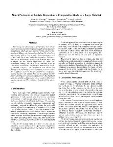
4 Experimental setup As mentioned above, the fundamental analytical tool that we will use is the learning curve. Learning curves represent the generalization performance of the models produced by a learning algorithm, as a function of the size of the training set. Figure 1 shows two typical learning curves. For smaller training{set sizes the curves are steep, but the increase in accuracy lessens for larger training{ set sizes. Often for very large training{set sizes this standard representation obscures small, but non{trivial, gains. Therefore to visualize the curves we will use two transformations. First we will use a log scale on the horizontal axis. Second, we will start the graph at the accuracy of the smallest training{set size (rather than at zero). The transformation of the learning curves in Figure 1 is shown in Figure 2. We produce learning curves based on 36 data sets. We now describe these data sets, the measures of error we use (for the vertical axes of the learning curve plots), the technical details of how learning curves are produced, and the implementations of the learning algorithms and variants.

12

Learning Curve of Californian Housing Data 0.9 0.8 0.7

Accuracy

0.6 0.5 0.4 0.3 0.2 0.1 Decision Tree Logistic Regression 0 0

2000

4000

6000

8000

10000

12000

14000

16000

Sample Size

Figure 1: Typical learning curves Learning Curve of Californian Housing Data 0.9 0.88 0.86

Accuracy

0.84 0.82 0.8 0.78 0.76 0.74 Decision Tree Logistic Regression 0.72 10

100

1000

10000

Sample Size

Figure 2: Log-scale learning curves 13

100000

4.1 Data sets

The 36 data sets in this study were selected to help achieve our goal of examining learning curves for tree induction and logistic regression, for the tasks of classication and ranking by probability of class membership. In order to get learning curves of a reasonable length, each data set was required to have at least 700 observations. To this end, we chose many of the larger data sets from the UCI data repository (Blake and Merz, 2000) and from other learning repositories. We selected data data drawn from real domains and avoided synthetic data. The rest were obtained from practitioners with real classication tasks with large data sets. The appendix gives source details for all the data sets. We only considered tasks of binary classication, which facilitates the use of logistic regression and allows us to compute the area under the ROC curve, described below, which we rely on heavily in the analysis. Some of the two{class data sets are constructed from data sets originally having more classes. For example, the Letter{A data set and the Letter{V data set are constructed by taking the UCI letter data set, and using as the positive class instances of the letter \a" or instances of vowels. Finally, because of problems encountered with some of the learning programs, and the arbitrariness of workarounds, we avoided missing data for numerical variables. If missing values occured in nominal values we coded them explicitly. C4.5 has a special facility to deal with missing values, coded as \?". In order to keep logistic regression and tree induction comparable, we choose a dierent code and modeled missing values explicitly as a nominal value. Only two data sets contained missing numerical data (Downsize and Firmreputation). In those cases we excluded rows or imputed the missing value using the mean for the column. For a more detailed explanation see the appendix. Table 1 shows the specication of the 36 data sets used in this study, including the maximum training size, the number of variables, the number of nominal variables, the total number of parameters (1 for a continuous variable, number of nominal values minus one. for each nominal variable), and the classication prior (the proportion of positive class instances in the training set).

4.2 Evaluation metrics

We compare performance using two evaluation metrics. First, we use classication accuracy (equivalently, undierentiated error rate): the number of correct predictions on the test data divided by the number of test data instances. This is the standard comparison metric used in studies of classier induction in the machine learning literature. Classication accuracy obviously is not an appropriate evaluation criterion for all classication tasks (Provost, Fawcett, and Kohavi, 1998). For this work we also want to evaluate and compare dierent methods with respect to their estimates of class probabilities. One alternative to classication accuracy is to use ROC (Receiver Operating Characteristic) analysis (Swets, 1988), which compares visually the classiers' performance across the entire range of proba14

Data set

Abalone Adult Ailerons Bacteria Bookbinder CalHous CarEval Chess Coding Connects Contra Covertype Credit Diabetes DNA Downsize Firm German IntCensor IntPrivacy IntShopping Insurance Intrusion Letter{A Letter{V Mailing Move Mushroom Nurse Optdigit Pageblock Patent Pendigit Spam Telecom Yeast

Table 1: Data sets

Max Training Variables Nominal Total Prior 2304 38400 9600 32000 3200 15360 1120 1600 16000 8000 1120 256000 480 320 2400 800 12000 800 16000 10900 12800 6400 256000 16000 16000 160000 2400 6400 10240 4800 4480 1200000 10240 3500 12800 1280

8 14 12 10 10 10 6 36 15 29 9 12 15 8 180 15 20 20 12 15 15 80 40 16 16 9 10 22 8 64 10 6 16 57 49 8

15

0 8 0 8 0 0 6 36 15 29 7 2 8 0 180 0 0 17 7 15 15 2 6 0 0 4 10 22 8 0 0 2 0 0 0 0

8 105 12 161 10 10 21 36 60 60 24 54 35 8 180 15 20 54 50 78 78 140 51 16 16 16 70 105 23 64 10 447 16 57 49 8

0.5 0.78 0.5 0.69 0.84 0.5 0.7 0.5 0.5 0.91 0.93 0.7 0.5 0.65 0.5 0.75 0.81 0.7 0.58 0.62 0.6 0.83 0.8 0.96 0.8 0.94 0.5 0.5 0.66 0.9 0.9 0.57 0.9 0.6 0.62 0.7

bilities. For a given binary classier that produces a score indicating likelihood of class membership, its ROC curve depicts all possible tradeos between true{ positive rate (TP ) and false{positive rate (FP ). Specically, any classication threshold on the score will classify correctly an expected percentage of truly positive cases as being positive (TP ) and will classify incorrectly an expected percentage of negative examples as being positive (FP ). The ROC curve plots the observed TP versus FP for all possible classication thresholds. Provost and Fawcett (Provost and Fawcett, 1997, 1998) describe how precise, objective comparisons can be made with ROC analysis. However, for the purpose of this study, we want to evaluate the class probability estimates generally rather than under specic conditions or under ranges of conditions. In particular, we will concentrate on how well the probability estimates can rank cases by their likelihood of class membership. There are many applications where such ranking is more appropriate than binary classication. Knowing nothing about the task for which they will be used, which probabilities are generally better for ranking? In the standard machine learning evaluation paradigm, the true class probability distributions are not known. Instead, a set of instances is available, labeled with the true class, and comparisons are based on estimates of performance from these data. The Wilcoxon({Mann{ Whitney) nonparametric test statistic is appropriate for this comparison (Hand, 1997). The Wilcoxon measures, for a particular classier, the probability that a randomly chosen class 0 case will be assigned a higher class 0 probability than a randomly chosen class 1 case. Therefore higher Wilcoxon score indicates that the probability ranking is generally better (there may be specic conditions under which the classier with a lower Wilcoxon score is preferable). Note that this evaluation side{steps the question of whether the probabilities are well calibrated.4 Another metric for comparing classiers across a wide range of conditions is the area under the ROC curve (AUR) (Bradley, 1997) AUR measures the quality of an estimator's classication performance, averaged across all possible probability thresholds. The AUR is equivalent to the Wilcoxon statistic (Hanley and McNeil, 1982), and is also essentially equivalent to the Gini coe"cient (Hand, 1997). Therefore, for this work we will report the AUR when comparing class probability estimators. It is important to reiterate that AUR judges the relative quality of the entire probability{based ranking. It may be the case that for a particular threshold (e.g., the top 10 cases) a model with a lower AUR in fact is desirable.

4 An inherently good probability estimator can be skewed systematically, so that although the probabilities are not accurate, they still rank cases equivalently. This would be the case, for example, if the probabilities were squared. Such an estimator will receive a high Wilcoxon score. A higher Wilcoxon score indicates that, with proper recalibration, the probabilities of the estimator will be better. Probabilities can be recalibrated empirically, for example as described by Sobehart et al. (2000) and by Zadrozny and Elkan (2001).

16

4.3 Learning Curves

In order to obtain a smooth learning curve with a maximum training size Nmax and test size T we perform the following steps 10 times and average the resulting curves. (1) Draw an initial sample Sall of size Nmax + T from the original data set. (We choose the test size T to be between one{quarter and one{third of the original size of the dataset.) (2) Split the set Sall randomly into a test set Stest of size T and keep the remaining Nmax observations as a data pool Strain-source for training samples. (3) Set the initial training size N to approximately 5 times the number of parameters in the logistic model. (4) Sample a training set Strain with the current training size N from Strain-source . (5) Remove all data from the test set Stest that have nominal values that did not appear in the training set. Logistic regression requires the test set to contain only those nominal values that have seen been previously in the training set. If the training sample did not contain the value \blue" for the variable color, for example, logistic regression cannot estimate a parameter for this dummy variable and will produce an error message and stop execution if a test example with color = \blue" appears. In comparison C4.5 splits the example probabilistically, and sends weighted (partial) examples to descendent nodes for details see Quinlan (1993). We therefore remove all test examples that have new nominal values from Stest and create Stest,N for this particular N . The amount of data rejected in this process depends on the distribution of nominal values, and the size of the test and current training set. However, we usually lose less than 10% of our test set. (6) Train all models on the training set Strain and obtain their predictions for the current test set Stest,N set. Calculate the various evaluation criteria for all models. (7) Repeat steps 3 to 6 for increasing training size N up to Nmax All samples in the outlined procedure are drawn without replacement. After repeating these steps 10 times we have for each method and for each training{set size 10 observations of all evaluation criteria. The nal learning curves of the algorithms in the plots connect the means of the replicated evaluation criteria values for each training{set size. We use the standard deviation of the replicated value as a measure of the inherent variability of each evaluation criterion across dierent training sets of the same size, constructing error bars at each training{ set size representing  one standard deviation. In the evaluation we will consider 17

two models as dierent for a particular training{set size if the mean for neither falls within the error bars of the other. We train all models on the same training data in order to reduce variation in the performance measures due to sampling of the training data. By the same argument we also use the same test set for all dierent training{set sizes (for each of the ten learning curves), as this decreases the variance and thereby increases the smoothness of the learning curve. It is important to note that since the evaluation criteria are based on a randomly sampled test set, any time-related structure that is present in the data is ignored in the evaluation. That is, none of the results reported here relate to performance of these methods in a forecasting situation, where observations from earlier points in time are used to predict values from later time periods. Forcasting is a very dierent situation from the one studied here, since in that context the possibility of the underlying relationships in the population changing over time is an important concern.

4.4 Implementation 4.4.1 Tree induction

To build classication trees we used C4.5 (Quinlan, 1993) with the default parameter settings. To obtain probability estimates from these trees we used the frequency scores at the leaves. Our second algorithm, C4.5-PET (Probability Estimation Tree), uses C4.5 without pruning and estimates the probabilities as Laplace{corrected frequency scores, as discussed in Section 3.1.2. The third algorithm in our comparison, BPET, performs a form of bagging (Breiman, 1996) using C4.5. Specically, averaged{bagging estimates 10 trees from 10 bootstrap subsamples of the training data and predicts the mean of the probabilities.5 Details of the implementations are summarized in Table 2.

4.4.2 Logistic Regression

Logistic regression was performed using the SAS program PROC LOGISTIC. A few of the data sets exhibited quasicomplete separation, in which there exists a linear combination of the predictors
0 x such that
0 xi 0 for all i where yi = 0 and
0 xi 0 for all i where yi = 1, with equality holding for at least one observation with yi = 0 and at least one observation with yi = 1. In this situation a unique maximum likelihood estimate does not exist, since the log{likelihood increases to a constant as at least one parameter becomes innite. Quasicomplete separation is more common for smaller data sets, but it also can occur when there are many qualitative predictors that have many nominal values, as is sometimes the case here. SAS stops the likelihood iterations prematurely with an error ag when it identies quasicomplete separation (So,

5 This is in contrast to standard bagging, for which votes are tallied from the ensemble of models and the class with the majority/plurality is predicted. Averaged{bagging allows us both to perform probability estimation and to perform classi cation (thresholding the estimates at 0 5). :

18

Table 2: Implementation Details

Name

C4.5 C4.5{PET BPET LR AIC Ridge BLR

Description of Probability Estimation

Frequency estimates on pruned tree Laplace corrected frequency estimates on unpruned tree 10{fold averaged-bagging of Laplace corrected frequency estimates on unpruned tree Multiple logistic regression Logistic regression with variable selection based on minimal AIC Ridge logistic regression 10{fold averaged-bagging of ordinary logistic regression

1995), which leads to inferior performance. For this reason, for these data sets the logistic regression models are t using the glm() function of R (Ihaka and Gentleman, 1996), since that package continues the maximum likelihood iterations until the change in log{likelihood is below a preset tolerance level. For bagged logistic regression, similarly to bagged tree induction, we used 10 subsamples with replacement of the same size as the original training set. We estimated 10 logistic regression models and took the mean of the probability predictions on the test set of those 10 models as the nal probability prediction for the test set. The issue of novel nominal values in the test set again creates problems for bagged logistic regression. As was noted earlier, logistic regression requires all levels of nominal variables that appear in the test set to have also appeared in the training set. In order to guarantee this for each of the 10 sub{ training sets, a base set was added to the 10 sub{training sets. This base set contains at least two observations containing each nominal value appearing in the test set. The variable selection variant and the ridge logistic regression were implemented in R. Due to computational constraints such as memory limits, these variants do not execute for very large data sets and so we can only report the basic logistic regression for those cases. Details of the implementation are summarized in Table 2.

5 Variants of methods: Learning curve analysis In this section we investigate the usefulness of the dierent variants of the algorithms discussed in Section 3. We rst focus on tree induction and then consider logistic regression.

19

5.1 Variants of tree induction

We compare the learning curves to examine the eects of pruning, the Laplace correction, and bagging. Pruning was introduced (and improved upon) in order to increase the accuracy of unpruned classication trees. Accuracy{based pruning (as in C4.5) can hurt probability estimation based on trees, because it eliminates distinctions in estimates that would not aect classication. For example, two sibling leaves with probability estimates of 0.8 and 0.9 both would yield a positive classication however, the dierent scores may improve ranking performance signicantly. The Laplace correction makes up for errors in scores due to the smaller samples at the leaves of unpruned trees, and due to the overly extreme bias in the probabilities, as discussed earlier. Bagging reduces variance, which leads to estimation errors as well as classication errors (Friedman, 1997). The ability of Laplace correction and bagging to improve probability estimation of induced trees has been noted previously. Bauer and Kohavi (1999) show improvements using mean{squared error from the true (0/1) class Provost, Fawcett, and Kohavi (1998) present ROC curves that show similar results, and Provost and Domingos (2000) show similar results using AUR. Our results are consistent with expectations.

Pruning (C4.5 versus PET)

For classication accuracy, pruning6 improves the performance in ten cases (wintie-loss tally: 10-25-1). However, the improvements are small in most cases. The top plot of Figure 3 shows a typical case of accuracy learning curves (Spam data set). The performance comparison of C4.5 and C4.5{PET is systematically reversed for producing ranking scores (AUR). The Laplace transformation/notpruning combination improves the AUR in twenty-two cases and is detrimental in only two cases (IntPriv and IntCensor) (win-tie-loss: 22-12-2). The lower plot of gure 3 shows this reversal on the same data set (Spam). Notice that, in contrast to accuracy, the dierence in AUR is considerable between C4.5 and C4.5{PET.

Bagging (BPET versus C4.5)

Averaged-bagging often improves accuracy, sometimes substantially. The wintie-loss tally is 10-21-5 in favor of bagging over C4.5. In terms of producing ranking scores (AUR), BPET was never worse than C4.5, with a 24-12-0 result.

Bagging (BPET versus C4.5{PET)

The only dierence between BPET and C4.5{PET is the averaged-bagging. Both use Laplace correction on unpruned trees. BPET dominates this comparison for both accuracy and probability estimation (16-18-2 for accuracy and

6 Recall that the Laplace correction will not change the classi cation decision, so the only dierence between C4.5 and C4.5{PET for classi cation is pruning.

20

0.96

0.94

Accuracy

0.92

0.9

0.88

0.86

0.84 BPET C4.5-PET C4.5 0.82 100

1000

10000

Sample Size 1

0.98

0.96

0.94

AUR

0.92

0.9

0.88

0.86

0.84

0.82 100

BPET C4.5-PET C4.5 1000

10000

Sample Size

Figure 3: Accuracy and AUR learning curves for Spam data set, illustrating performance of variants of probability estimation trees. 21

15-19-2 for AUR). The two data sets where bagging hurts are Mailing and Abalone. However, looking ahead, in both these cases tree induction did not perform well compared to logistic regression. Based on these results, for the comparison with logistic regression in Section 6, we will use two methods: C4.5{PET (Laplace corrected and not pruned) and BPET. Keep in mind that this may underrepresent C4.5's performance slightly when it comes to classication accuracy, since with pruning regular C4.5 typically is slightly better. However, the number of runs in Section 6 is huge. Both for comparison and for computational practicability it is important to limit the number of learning algorithms. Moreover, we report surprisingly strong results for C4.5 below, so our choice here is conservative.

5.2 Variants of logistic regression

In this section we discuss the properties of the three variants of logistic regression that we are considering. Model selection using AIC sometimes results in improved performance relative to using the full logistic regression model, particularly for smaller sample sizes. Evidence of this is seen, for example, in the Adult, Bacteria, Mailing, Firm, German, Spam, and Telecom data sets. Figure 4, which shows the logistic regression accuracy learning curves for the Firm data set, gives a particularly clear example, where the AIC learning curve is consistently higher than that for ordinary logistic regression, and distinctly higher up to sample sizes of at least 1000. Corresponding plots for AUR are similar. Model selection also can lead to poorer performance, as it does in the CalHous, Coding, and Optdigit data sets. However, as was noted earlier, AIC -based model selection is infeasible for large data sets.7 The story for ridge logistic regression is similar, but less successful. While ridge logistic regression was occasionally eective for small samples (see, for example, Figure 5, which refers to the Intshop data set), for the majority of data sets using it resulted in similar or poorer performance compared to the full regression. We will therefore not discuss it further. Note, however, that we used one particular method of choosing the ridge parameter  perhaps some other choice would have worked better, so our results should not be considered a blanket dismissal of the idea of ridge logistic regression. We also found, perhaps surprisingly at rst, that bagging is systematically detrimental to performance for logistic regression. In fact, in contrast to the observation regarding bagging for trees, for logistic regression bagging seems to shift the learning curve to the right! Upon further consideration, this is not surprising. Bagging trains individual models with substantially fewer data

7 More speci cally, implementation of the Venables and Ripley (1999) AIC{based selector is based on the package R, and use of this package becomes infeasible for very large data sets There is an implementation for the package S{Plus, but this package is also not feasible for massive data sets We know of no implementation for SAS.

22

0.95

0.9

Accuracy

0.85

0.8

0.75

0.7 LR AIC Ridge 0.65 100

1000 Sample Size

10000

Figure 4: Accuracy learning curves of logistic regression variants for Firm reputation data set, illustrating stronger performance of model selection{based logistic regression for smaller sample sizes. 0.74

0.72

0.7

Accuracy

0.68

0.66

0.64

0.62

0.6

0.58

0.56 100

LR AIC Ridge 1000

10000

100000

Sample Size

Figure 5: Accuracy learning curves of logistic regression variants for Internet shopping data set, illustrating a situation where ridge logistic regression is effective for small sample sizes. 23

0.92

0.9

0.88

Accuracy

0.86

0.84

0.82

0.8

0.78 BLR LR 0.76 10

100

1000

Sample Size

Figure 6: Accuracy learning curves for Californian housing data set, illustrating the negative impact of bagging on logistic regression performance. (approximately 0:63n distinct original observations, where n is the trainingset size). Therefore when the learning curve is steep, the individual models will have considerably lower accuracies than the model learned from the whole training set. In trees, this eect is more than compensated for by the variance reduction, usually yielding a net improvement. However, logistic regression has little variance, so all bagging does is to average the predictions of a set of poor models (note that bagging does seem to result in a small improvement over the accuracy produced with 63% of the data). In sum, our conclusion for logistic regression is quite dierent from that for tree induction (in the previous section). For larger training{set sizes, which are at issue in this paper, none of the variants improve considerably on the basic algorithm. Indeed, bagging is detrimental. Therefore, for the following study we only consider the basic algorithm. It should be noted, however, that this decision has no eect on our conclusions concerning the relative eectiveness of logistic regression and tree induction, since for the smaller data sets the ranking of the basic logistic regression algorithm compared to tree induction is the same as that of the variants of logistic regression. One other general property of logistic regression learning curves is illustrated well by Figure 2|the leveling o of the curve as the size of the data set increases. In virtually every example examined here, logistic regression learning curves either had leveled o at the right end, or were in the process of doing so. This 24

is exactly what would be expected for any parametric model (including logistic regression). As the data set gets larger, eventually the parameters of the model are estimated as accurately as they can be, with standard error (virtually) zero. At this point additional data will not change anything, and the learning curve must level o.

6 Dierences between tree induction and logistic regression: Learning curve analysis We now present our main experimental analysis. We compare the learning curve performance of the three chosen methods, C4.5{PET (Laplace{corrected, unpruned probability estimation tree), BPET (bagged C4.5{PET), and multiple logistic regression, as tools for building classication models and models for class probability estimation. Here and below, we are interested in comparing the performance of tree induction with logistic regression, so we generally will not dierentiate in summary statements between BPET and PET, but just say \C4". In the graphs we show the performance of all the methods. Table 3 summarizes the results for our 36 data sets. As indicated by the rst column, each row corresponds to a data set. The second column (Winner AUR) indicates which method gave the best AUR for the largest training set. If the mean for one algorithm falls within the error bars for another, a draw is declared (denoted \none"). The next column (Winner Acc) does the same for classication accuracy. The third column indicates the maximum AUR for any method on this data set. We will explain this presently. The nal column summarizes the comparison of the learning curves. \X dominates" means that a method of type X outperforms the other method for all training{set sizes. \X crosses" indicates that a method of type X is not better for smaller training{set sizes, but is better for larger training{set sizes. \Indistinguishable" means that at the end of the learning curve with maximal training set we cannot identify one method (logistic regression or a tree induction) as the winner. One data set (Adult) is classied as \Mixed". In this case we found dierent results for Accuracy (C4 crosses) and AUR (LR dominates). We will discuss the reason and implications of this result more generally in Section 6.3. As described above, the area under the ROC curve (AUR) is a measure of how well a method can separate the instances of the dierent classes. In particular, if you rank the instances by the scores given by the model, the better the ranking the larger the AUR. A randomly shu%ed ranking will give an AUR of (near) 0.5. A perfect ranking (perfectly separating the classes into two groups) gives an AUR of 1.0. Therefore, AUR can be considered an estimated \signal{to{noise ratio," with respect to the modeling methods available. If no method does better than random (Max AUR = 0.5), then for our purposes there is no signal (and it doesn't make sense to compare learning algorithms). If some method performs perfectly (Max AUR = 1.0), then for our purposes there is no noise. AUR is better than classication accuracy for this purpose, 25

Table 3: Results of learning curve analyses.

Data set

Winner AUR Winner Acc Max AUR Result

Yeast

none

Nurse Mushrooms Optdigit Letter{V Letter{A Intrusion DNA Covertype Telecom Pendigit Pageblock CarEval Spam Chess CalHous Ailerons Firm Credit Adult Connects Move Downsize Coding German Diabetes Bookbinder Bacteria Patent

Contra

IntShop IntCensor Insurance

IntPriv Mailing Abalone

none none none C4 C4 C4 C4 C4 C4 C4 C4 none C4 C4 C4 none LR C4 LR C4 C4 C4 C4 LR LR LR none

none none none C4 C4 C4 C4 C4 C4 C4 C4 C4 C4 C4 C4 C4 LR C4 C4 none C4 C4 C4 LR LR LR C4

C4

C4

none

LR LR

none

LR LR LR

1 1 0.99 0.99 0.99 0.99 0.99 0.99 0.98 0.98 0.98 0.98 0.97 0.95 0.95 0.95 0.93 0.93 0.9 0.87 0.85 0.85 0.85 0.8 0.8 0.8 0.79

Indistinguishable Indistinguishable Indistinguishable C4 dominates C4 crosses C4 dominates C4 dominates C4 crosses C4 dominates C4 dominates C4 crosses C4 crosses C4 dominates C4 dominates C4 crosses C4 crosses LR crosses C4 dominates Mixed C4 crosses C4 dominates C4 crosses C4 crosses LR dominates LR dominates LR crosses C4 crosses

none

0.78 Indistinguishable

none

0.73 Indistinguishable

LR LR

none

none none LR

26

0.75 C4 crosses

0.7 LR crosses 0.7 LR dominates

0.7 Indistinguishable

0.66 LR crosses 0.61 LR dominates 0.56 LR dominates

1

0.995

0.99

0.985

AUR

0.98

0.975

0.97

0.965

0.96

0.955 100

LR BPET C4.5-PET 1000

10000

Sample Size

Figure 7: AUR learning curves for Optdigit data set, illustrating situation where all methods achieve high performance relatively quickly. because it is comparable across data sets. For example, it is not aected by the marginal (\prior") probability of class membership. A data set with 99.99% positive examples should engender classication accuracy of at least 99.99%, but still might have an AUR = 0.5 (there is no signal to be modeled). The data sets in Table 3 are presented in order of decreasing Max AUR|the easiest at the top, and the hardest at the bottom. We have separated the results in Table 3 into three groups, indicated by horizontal lines. The relative performance of the classiers appears to be fundamentally dierent in each group. The topmost group, comprising Mushroom, Nurse, and Optdigit, are three situations where the signal{to{noise ratio is extremely high. All methods quickly attain accuracy and AUR values over .99, and are indistinguishable. The learning curves for AUR for Optdigit are shown in Figure 7. For purposes of comparison, these data sets are \too easy," in the sense that all methods isolate the structure completely, very quickly. Since these data sets do not provide helpful information about dierences in eectiveness between methods, we will not consider them further. Remarkably, the comparison of the methods for the rest of the data sets can be characterized quite well by two aspects of the data: the level of noise in the data, and the size of the data set. As just described, we measure the level of noise using Max AUR. We split the measure to reect a high/low split: 27

1

0.95

Accuracy

0.9

0.85

0.8

0.75

0.7 LR BPET C4.5-PET 0.65 10

100

1000 Sample Size

10000

100000

Figure 8: Accuracy learning curves for Letter{V data set, illustrating situation where C4 dominates.

AUR :8 (lower signal{to{noise) versus AUR > :8 (higher signal{to{noise). The AUR split is reected in the lower, horizontal division in the table.

6.1 Data with high signal{to{noise ratio

The higher signal{to{noise ratio situation (AUR > :8) is clearly favorable for the trees. Of the 21 high{signal data sets, in 19 C4 is clearly better in terms of accuracy by the time the learning curve reaches its highest estimation point (C4's win{tie{loss record is 19-1-1). In some cases the tree dominates from the start Letter{V is a good example of this situation, as shown in Figure 8. Here the logistic regression learning curve is initially slightly steeper than that of the tree, but the logistic regression curve quickly levels o, while the tree keeps learning, achieving far higher accuracy than the logistic regression. Move, Pendigit, and Spam are roughly similar. In the other situations, logistic regression's advantage for smaller data sets extends further, so that it is clearly better for smaller data sets, but eventually tree induction surpasses logistic regression both in terms of accuracy and AUR. Ailerons, Coding, Covertype, and Letter{A provide good examples of this situation. The AUR curves for Covertype are shown in Figure 9. Interestingly, in all of these cases the crossover point is in the range of a training{set size of 1000{3000 observations. Thus, our results suggest that for higher signal{to{ noise situations, past a few thousand observations, it is unlikely that logistic regression will outperform probability trees. 28

1

0.95

0.9

AUR

0.85

0.8

0.75

0.7 BPET C4.5-PET LR 0.65 100

1000

10000 Sample Size

100000

1e+06

Figure 9: AUR learning curves for Covertype data set, illustrating situation where logistic regression is initially a better performer, but trees eventually dominate. It is natural to ask whether there are clear dierences between the dominating cases and the cases of crossing. We do not have a denitive answer, but it seems to be a combination of two factors. First, how \linear" is the problem. If there are few non{linearities and there is little noise, then logistic regression will do well from the beginning (relative to the number of parameters, of course) tree induction needs more data to reach the necessary complexity. Second, it simply depends on where you start looking: what is the smallest training{set size in relation to the number of parameters. If you start with a relatively high number, trees are likely to dominate. Are there dierences between the curves for classication (accuracy) and probability rank ordering (AUR) for this group of data sets? Table 3 shows that logistic regression is a bit more competitive for AUR than for accuracy (AUR win{tie{loss for C4.5 is 17-2-2). Generally, the shapes of the learning curves with respect to accuracy and AUR for a given data set are similar, but the accuracy curves are shifted to the left: C4.5 needs fewer data for classication than for probability estimation (again, not surprisingly). Therefore, when the C4.5 curve crosses the logistic regression curve, the crossover point for accuracy comes at the same point or later than the crossover point for AUR, but not earlier. An alternative view is that logistic regression apparently is better tuned for probability ranking than it is for classication. Given that the method is specically designed to model probabilities (with classication as a possible side{eect of that probability estimation), this also is not surprising. 29

Evidence of this can be seen in Adult, Ailerons, and Letter{A, where the crossover point of the AUR learning curves has not been reached (although the trajectories of the curves suggest that with more data the tree would eventually become the winner). The cases for Adult for both accuracy and AUR are shown in Figure 10.

6.2 Data with low signal{to{noise ratio

The lower signal{to{noise ratio situation (AUR :8) is slightly more complicated. Sometimes it is impossible to distinguish between the performances of the methods. Examples of this (italicized in Table 3) include Contraception, Insurance and Yeast. For these data sets it is di"cult to draw any conclusions, in terms of either accuracy or AUR, since the curves tend to be within each other's error bars. Figure 11 illustrates this for the Contra data set. When the methods are distinguishable logistic regression is clearly the more eective method, in terms of both accuracy and AUR. Ten data sets fall into this category. Logistic regression's win{tie{loss record here is 8-1-1 for AUR and 6-2-2 for accuracy. Examples of this are Abalone, Bookbinder, Diabetes, and the three Internet data sets (IntCensor, IntPrivacy, and IntShopping). Figure 12 shows this case for the IntCensor data set. As was true in the higher signal{to{noise situation, logistic regression fares better (comparatively) with respect to AUR than with respect to accuracy. This is reected in a more clear gap between logistic regression and the best tree method in terms of AUR compared to accuracy see, for example, the results of IntPriv and the Mailing data where logistic regression wins for AUR, but not for accuracy.

6.3 The Impact of Data Set Size

The Patent data set is an intriguing case, which might be viewed as an exception. In particular, although it falls into the low signal{to{noise category, C4 is the winner for accuracy and for AUR. This data set is by far the largest in the study, and at an extremely large training data size the induced tree becomes competitive and beats the logistic model. As shown in Figure 13, the curves cross when the training sets contain half a million examples or more. This is consistent with the common view that machine learning tools are better suited for large data sets than statistical tools, but note that in this case \large" means truly massive from the perspective of statistical analyses. The impact of data-set size on these results is twofold. First, in this study we use the maximum AUR as a proxy for the signal{to{noise ratio. However, even with our large data sets, in almost no case did the AUR learning curve level o for tree induction. This suggests that we tend to underestimate the signal{to{noise ratio. The second impact of data-set size concerns conclusions about which method is superior. We have 15 cases where the curve for one method crosses the other as the training-set size increases, and some of the mixed cases show that 30

0.87 0.86 0.85 0.84

Accuracy

0.83 0.82 0.81 0.8 0.79 LR BPET C4.5-PET

0.78 0.77 100

1000

10000

100000

Sample Size 0.92

0.9

AUR

0.88

0.86

0.84

0.82 LR BPET C4.5-PET 0.8 100

1000

10000

100000

Sample Size

Figure 10: Accuracy and AUR learning curves for Adult data set, illustrating the later crossover of the tree curves past the logistic regression curves for AUR compared to accuracy. 31

0.8

0.75

AUR

0.7

0.65

0.6 LR BPET C4.5-PET 0.55 10

100

1000

10000

Sample Size

Figure 11: AUR learning curves for Contra data set, illustrating low signal{to{ noise and indistinguishable performance. one method is dominated for small training size but later reaches the same performance level. In all of those cases the conclusion about which method is better would have been dierent if only a smaller sample of the data had been available.

7 Discussion and Implications These results show that considering training{set size in a comparison of classier induction algorithms (i.e., examining learning curves on large data sets) can help us to understand dierences in performance. Let us consider the results in the context of prior work. The most comprehensive experimental study of the performance of induction algorithms (that we know of) is described by Lim, Loh, and Shih (2000). They show that averaged over 32 data sets, logistic regression out-performs C4.5. Specically, the classication error rate for logistic regression is 7% lower than that of C4.5. Additionally, logistic regression was the second best algorithm in terms of consistently low error rates: it is not signicantly dierent from the minimum error rate (of the 33 algorithms they compare) on 13 of the 32 data sets. The only algorithm that fared better (15/32) was a complicated spline{based logistic regression that was extremely expensive computationally. In comparison, C4.5 was the 17th best algorithm in these 32

0.74 0.72 0.7 0.68 0.66

AUR

0.64 0.62 0.6 0.58 0.56 LR BPET C4.5-PET

0.54 0.52 100

1000

10000

100000

Sample Size

Figure 12: AUR learning curves for IntCensor data set, illustrating situation where logistic regression dominates. terms, not diering from the minimum error rate on only seven of the data sets. Our results clarify and augment the results of that study. In particular, Lim et al. concentrate on UCI data sets without considering data{set size. Their training{set sizes are relatively small specically, their average training{set size is 900 (compare with an average of 60000 at the right end of the learning curves of the present study median=12800).8 Although C4.5 would clearly win a straight comparison over all the data sets in our study, examining the learning curves shows that C4.5 often needs more data than logistic regression to achieve its ultimate classication accuracy. This leads to a more general observation, that bears on many prior studies by machine learning researchers comparing induction algorithms on xed{size training sets. In only 14 of 36 cases does one method dominate for the entire learning curve (and therefore training{set size does not matter). Thus, it is not appropriate to conclude from a study with a single training{set size that one algorithm is \better" (in terms of predictive performance) than another for a particular domain. Rather, such conclusions must be tempered by examining whether the learning curves have reached plateaus. If not, one only can conclude that for the particular training{set size used, one algorithm performs better than 8 Furthermore, 16 of their data sets were created by adding noise to the other 16. However, from their analysis we can not conclude that this is the reason for the dominance of logistic regression.

33

0.8

0.75

AUR

0.7

0.65

0.6

0.55 BPET C4.5-PET LR 0.5 100

1000

10000 100000 Sample Size

1e+06

1e+07

Figure 13: AUR learning curves for the Patent data set, illustrating the situation where tree induction surpasses logistic regression for extremely large training{ set sizes. another. In this study of two learning methods, each the de facto standard in statistics or in machine learning, we can see clear criteria for when each algorithm is preferable: C4 for low{noise data and logistic regression for high{noise data. Curiously, the two clear exceptions in the low signal{to{noise case (the cases where C4 beats logistic regression), Patent and Bacteria, may not be exceptions at all it may simply be that we still do not have enough data to draw a nal conclusion. For both of these cases, the C4 learning curves do not seem to be leveling o even at the largest training{set sizes. Figure 13 shows this for the Patent data set and Figure 14 shows this for the Bacteria data set. In both cases, given more training data, the maximum AUR may well exceed 0.8 in other words, these data may actually fall into the high signal{to{noise category. If that were so, the C4{tie{LR record for accuracy for the high{signal data sets would be 21-1-1, and for the (large{enough) low{signal data sets 0-2-6. Why is there a connection between relative performance and noise level? At this point, we can only speculate. It seems safe to assume that the world does not provide us solely with linear problems. Therefore, when noise is low, the highly nonlinear nature of tree induction allows it to identify and exploit complex structure that logistic regression misses. On the other hand, when noise is high, the massive search performed by tree induction algorithms leads them to identify noise as signal, resulting in a deterioration of performance. It 34

0.85

0.8

0.75

0.7

AUR

0.65

0.6

0.55

0.5

0.45

0.4 100

LR BPET C4.5-PET 1000

10000

100000

Sample Size

Figure 14: AUR learning curves for Bacteria data set. The AUR of Bacteria has already reached 0.79 and tree induction has not leveled o. One could speculate that BPET will achieve AUR>0.8. is a statistical truism that \All models are wrong, but some are useful" (Box, 1979, p. 202) this is particularly true when the data are too noisy to allow identication of the \correct" relationship. The general curve-crossing patterns we see concur with prior simulation studies showing learned linear models outperforming more complex learned models for small data sets, even when the more complex models better represent the true concept to be learned (Flury and Schmid, 1994 Domingos and Pazzani, 1997). A limitation of our study is that we used the default parameters of C4.5. For example, the \-m" parameter species when to stop splitting, based on the size of leaves. Quinlan (1993) notes that the default value may not be best for noisy data. Therefore, one might speculate that with a better parameter setting, C4.5 might be more competitive with logistic regression for the highnoise data. Although the focus of this paper was the \o-the-shelf" algorithms, we have experimented systematically with the \-m" parameter on a large, highnoise data set (Mailing). The results do not draw our current conclusions into question. How can these results be used by practitioners with data to analyze? The results show convincingly that learning curves must be examined if experiments are being run on a dierent training{set size than that which will be used to produce the production models. For example, a practitioner typically experiments on data samples to determine which learning methods to use, and then scales up the analysis. These results show clearly that this practice can be misleading 35

0.9

0.88

0.86

Accuracy

0.84

0.82

0.8

0.78

0.76

0.74 LR BPET Hybrid: LR -> BPET 0.72 10

100

1000

10000

100000

Sample Size

Figure 15: Accuracy learning curves for a hybrid model on the California Housing data set. for many domains, if the relative shapes of the learning curves are not taken into account as well. We also believe that the signal{to{noise categorization can be useful, in cases where one wants to reduce the computational burden of comparing learning algorithms on large data.9 In particular, consider the following strategy. 1. Run C4.5{PET with the maximally feasible training{set size. For example, use all the data available or all that will run well in main memory. C4.5 typically is a very fast induction alternative (cf., Lim, Loh, and Shih, 2000). 2. If the resultant AUR is high (0.8 or greater) continue to explore tree{based (or other nonparametric) options (e.g., BPET, or methods that can deal with more data than can t in main memory (Provost and Kolluri, 1999)). 3. If the resultant AUR is low, try logistic regression. An alternative strategy is to build a hybrid model. Figure 15 shows the performance of tree induction on the California Housing data set, where tree building takes the probability estimation from a logistic regression model as an additional input variable. Note that the hybrid model tracks with each model

9 For example, we found during this study that, depending on what package is being used, logistic regression often takes an excessively long time to run, even on moderately large data sets.

36

in its region of dominance. In fact, around the crossing point, the hybrid model is substantially better than either alternative. Another limitation of this study is that by focusing on the AUR, we are only examining probability ranking, not probability estimation. Logistic regression could perform better in the latter task, since that is what the method is designed for.

8 Conclusion We have used learning curves to study the eectiveness of tree induction and logistic regression for classication and probability ranking. In the paper's introduction we stated three related goals of our investigation, all involving the comparison of tree induction and logistic regression. The results of the learning curve analysis have provided us with considerable insight into the relative performance of the methods. By using real data sets of very dierent sizes, with dierent levels of noise, we have been able to identify several broad patterns in the performance of the methods. In particular, we see that the highly nonlinear nature of trees allows tree induction to exploit structure when the noise level in the data is low. On the other hand, the smoothness (and resultant low variance) of logistic regression allows it to perform well when noise is high. Within the logistic regression family, we see that once the training sets are reasonably large, standard multiple logistic regression is remarkably robust, in the sense that dierent variants we tried do not improve performance (and bagging hurts performance). In contrast, within the tree induction family the dierent variants continue to make a dierence across the entire range of training{set sizes: bagging usually improves performance, pruning helps for classication, and not pruning plus Laplace smoothing helps for scoring.10 We also have shown that examining learning curves is essential for comparisons of induction algorithms in machine learning. Without examining learning curves, claims of superior performance on particular \domains" are questionable at best. To emphasize this point, we calculated the C4{tie{LR records that would be achieved on this (same) set of domains, if data{set sizes had been chosen particularly well for each method. For accuracy, choosing well for C4 we can achieve a record of 22-13-1. Choosing well for LR we can achieve a record of 8-14-14. Similarly, for AUR, choosing well for C4 we can achieve a record of 23-11-2. Choosing well for LR we can achieve a record of 10-9-17. Therefore, it clearly is not appropriate, from simple studies with one data{set size (as with most experimental comparisons), to draw conclusions that one algorithm is better than the other for the corresponding domains. These results also call into question the practice of experimenting with smaller data sets (for e"ciency reasons) to choose the best learning algorithm, 10 On the other hand, the tree{learning program (C4.5, that is) is remarkably robust when it comes to running on dierent data sets. The logistic regression packages require much more hand{holding.

37

and then \scaling up" the learning with the chosen algorithm. The apparent superiority of one method over another for one particular sample size does not necessarily carry over to larger samples (from the same domain). Similarly, conclusions from experimental studies conducted with certain training{set/test{set partitions (e.g., two{thirds/one{third) many not even generalize to the source data set! Consider Patent, as shown in Figure 13. A corollary observation is that tree{induction learning curves usually do not plateau, even for very large data sets. Catlett (1991) concluded that learning curves do not plateau, on several large{at{the{time data sets (the largest with fewer than 100
000 training examples).11 Provost and Kolluri (1999) suggest that this conclusion should be revisited as the size of data sets that can be processed (feasibly) by learning algorithms increases. Our results provide a contemporary reiteration of Catlett's. On the other hand, our results seemingly contradict conclusions or assumptions made in some prior work. For example, Oates and Jensen (1997) conclude that classication{tree learning curves plateau, and Provost et al. (1999) replicate this nding and use it as an assumption of their sampling strategy. Technically, the criterion for a curve to have reached a plateau in these studies is that there be less than a certain threshold (one percent) increase in accuracy from the accuracy with the largest data{set size however, the conclusion often is taken to mean that increases in accuracy cease. Our results show clearly that this latter interpretation is not appropriate. Finally, before undertaking this study, we had expected to see crossings in curves|in particular, to see the tree induction's relative performance improve for larger training{set sizes. We had no idea we would nd such a clean{cut characterization of the performance of the learners in terms of the data sets' signal{to{noise ratios. Neither did we expect such clear evidence that the notion of how large a data set is must take into account the noisiness of the data. Looking forward, we believe that reviving the learning curve as an analytical tool in machine learning research can lead to other important, perhaps surprising insights.

Acknowledgments We thank Batia Wiesenfeld, Rachelle Sampson, Naomi Gardberg, and all the contributors to (and librarians of) the UCI repository for providing data. We also thank Tom Fawcett for writing and sharing the BPET software, Ross Quinlan for all his work on C4.5, Pedro Domingos for helpful discussions about inducing probability estimation models, and IBM for a Faculty Partnership Award. PROC LOGISTIC software is copyright, SAS Institute Inc. SAS and all other SAS Institute Inc. product or service names are registered trademarks or trademarks of SAS Institute Inc., Cary, NC, USA. 11

Note that Catlett's large data set was free of noise.

38

A Appendix: Data sets Adult

This census income database was donated by Ron Kohavi to the UCI repository. The task is to predict whether income exceeds $50K/yr based on census data. We have selected a subset of 14 variables with the main goal to reduce the complexity of the problem but not with specic attention towards the predictive power of a variable.

Ailerons

This data set addresses a control problem, namely ying an F16 aircraft. The attributes describe the status of the airplane, while the goal is to predict the discretized control action on the aileron of the aircraft. This data set can be obtained from the RT homepage at http://www.ncc.up.pt/ltorgo/RT.

Bacteria

This data set is extracted from a hospital information system in a municipal hospital, which includes information about clinical environments, names of detected bacteria, and characteristics of detected bacteria. This data was used in the KDD Challenge 2000 at the Fourth Pacic{Asia Conference on Knowledge Discovery and Data Mining (PAKDD2000) and was donated by Dr. Shusaku Tsumoto from the Department of Medical Informatics, Shimane Medical University. We selected a subset of 10 variables since most of the original 161 variables contained many missing data, and we predict whether bacteria were found or not.

Bookbinder

This data set comes as an example with the Marketing Engineering Software by G. Lilien and A. Rangaswamy (http://www.mktgeng.com). The task is to predict the choice of a customer based on previous shopping activity.

Californian Housing

This data can be found on the RT homepage by L. Torgo. The original task is to predict the price of a house with a given specication. We discretized the output variable in to > $130000 and $130000 to form a classication task.

Car Evaluation

This UCI data set is special since it has for each possible combination of nominal values of the variables (all six are categorical) exactly one output, acceptable or not acceptable. It was derived from a simple hierarchical decision model.

39

Chess

This is a UCI data set that represents chess end{games. It has six nominal attributes and the classication task is to predict whether the player won or did not win.

Coding

The protein coding region (PCR) data set (courtesy of Craven and Shavlik, 1993) contains DNA nucleotide sequences and their binary classications (coding or noncoding). Each sequence has 15 nucleotides with four dierent values per nucleotide. If the 15 nucleotides represent 5 codons which are part of a known protein, the sequence is labeled coding.

Connect

This data set was donated to the UCI collection by John Tromp. The task is to classify from legal 8{ply positions of a connect{4 game whether the player wins or loses. We excluded the 3rd class of draw from the original data set as well as nominal variables with fewer than 10 instances for any of their values.

Contraception

This data set is a subset of the 1987 National Indonesia Contraceptive Prevalence Survey and is available from the UCI collection. The subjects are married women who were either not pregnant or did not know if they were pregnant at the time of interview. The problem is to predict the current contraceptive method choice (no use or use) of a woman based on her demographic and socioeconomic characteristics.

Covertype

This is one of the largest UCI classication data sets with originally more than 500,000 observations. The data were donated by Jock A. Blackard and Colorado State University. The goal is to classify the forest cover type (tree type) based on cartographic variables. We keep only the two main classes of the original seven tree types in our sample: Spruce{Fir and Lodgepole Pine, which together accounted for 85% of the data.

Credit

This data set was donated by J.R. Quinlan and can be obtained from the UCI repository or from the StatLog project under the name Australian Credit Approval. The goal is to predict credit approval. There is no detailed information about the meaning of the input variables available, all attribute names and values have been changed to meaningless symbols to protect condentiality of the data. 40

Mailing{KDD Cup 98

This data set was used in the 1998 KDD Cup and is available from UCI. The objective of the analysis is to identify response to a fundraising campaign by a nonprot organization. For our study we selected a preprocessed subset of nine demographic and historical response variables based on the reports of the Cup winners.

Diabetes

This data set was used in the StatLog project and can be found at http://www.liacc.up.pt/ML/statlog/data sets.html. The task is to predict whether a patient tests positive for diabetes based on eight personal and clinical variables.

DNA

This data set was originally called Splice and is part of the UCI Molecular Biology data set. The goal is to classify a sequence of 60 nucleotides as boundary elements or nonboundary. There are two types of boundary elements: donors and acceptors which we combined for our classication goal into one category. The 60 nucleotides are coded as 3 binary dummies for the 4 possible nucleotides.

Downsize

This data set was created for a study by Wiesenfeld, Brockner, and Martin (1999) on the perception of fairness in organizational downsizing. We use a subset of 15 questions about the perceived procedural justice of the downsizing with response levels from 1{7 (\very little" to \a great deal") to predict the response of general job satisfaction. The predictors are treated as numerical variables. Records with more than three missing values where excluded. For up to three missing values per record we substituted the mean of the record, based on the observation that there was a high correlation between the variables.

Firm Reputation

The data set from the RQGold 2000 survey was sponsored by the Reputation Institute and conducted by Harris International (Fombrun, Gardberg, and Sever, 2000). The classication task is to predict whether the response to the overall reputation rating of a company is greater than 3 given a scale from 1 (equals \very bad" reputation) to 7 (equals \very good" reputation). As independent variables we used the responses to 17 questions that classied the company in terms of innovation, competitiveness, protability and so on. Those variables were on a 1{7 scale from \Does not describe the company" to \Describes the company very well." As was the case for the Downsize data, we treated the variables as numerical and replaced up to three missing values by the observation mean. 41

German Credit

This StatLog data set is similar to the Credit data set, where a classication of credit approval is based on personal information, banking information, purpose of credit, and previous credit.

Insurance

The Insurance Company Benchmark was used in the CoIL 2000 Challenge and contains information on customers of an insurance company. The data consists of 86 variables and includes product usage data and socio{demographic data derived from geographic codes. The classication task is to predict whether a customer would be interested in buying a caravan insurance policy.

Internet Censor

This data was derived from parts of a survey conducted by the Graphics and Visualization Unit at Georgia Tech from October 10 to November 16, 1997. The full details of the survey are available at http://www.cc.gatech.edu/gvu/user surveys/survey-1997-10/. The task is to predict the subject's position on Internet censorship based on personal information and political position.

Internet Privacy

This data set comes from the same survey as Internet Censor but from a dierent section with focus on use of personal data provided by the visitor of a site for personalization and direct marketing.

Internet Shop

This is another data set derived from the 1997 Internet survey from GVU. The focus of this section was the willingness to use online shopping based on browsing behavior and general use of the Internet for information, news, nancial services.

Intrusion/KDD Cup 99

This data set was used for The Third International Knowledge Discovery and Data Mining Tools Competition, and is available from the UCI repository. The competition task was to classify computer connection into the internal system into bad connections, called intrusions or attacks, and normal connections.

Letter{A

The objective of this UCI data set is to identify one (A) of the 26 capital letters in the English alphabet based on 16 mathematically derived features of the digital image. 42

Letter{V

This is the same data set as Letter{A but now the task is to identify vowels.

Move

This data set was originally used by William Cohen at AT&T. The task is to classify video game moves as random or not random. A more detailed description is given by Cohen (1995).

Mushrooms

This UCI data set classies mushrooms into denitely edible or potentially poisonous by combining the original three classes of denitely poisonous, unknown edibility and not recommended into potentially poisonous. The independent variables are mushroom features such as color, size, and shape.

Nurse

The Nursery data set was derived from a hierarchical decision model originally developed to rank applications for nursery schools based on occupation of parents and child's nursery, family structure and nancial standing, and social and health picture of the family. The data are available from the UCI repository.

Optdigit

The UCI optical digit recognition data were modied to a binary classication task by categorizing the output as 0 or other. The data are based on normalized bitmaps of hand written digits.

Pageblock

The problem in this UCI data set consists of classifying all the blocks of the page layout of a document that has been detected by a segmentation process. Originally the problem had ve classes: text, pictures, graphic, horizontal, and vertical lines. The binary classication task is to distinguish between text and nontext sections based on heights, length and area of the block, and measures of the distribution of black pixels.

Patent

This data set is the most complex and with two million observations the largest one used for this study. The data are issued by the U.S. Patent and Trademark O"ce to Micropatent. It contains the information from the front page of every patent granted since 1975. We selected a subset of the available variables: year, country origin, number of assignees, U.S. classication code, and number of US references. To reduce the complexity we grouped the country of origin into six categories: U.S., Europe, Canada, Australia, Japan and Other. The 43

classication task is to predict whether this patent has received international references.

Pendigit

This UCI data set is similar to the Optdigit data. The goal is to classify handwritten digits as 0 or not 0 based on sampled x and y input coordinates from a pressure sensitive table.

Spam

This collection of e{mails is also part of the UCI collection. The goal is to build a spam lter that identies spam mail like advertisements, chain letters and pornography based on features like: frequent words, consecutive capital letters, total number of capital letters and so on.

Telecom

This is a commercial application described in Weiss and Indurkhya (1995). The data describe a telecommunication problem and can be found at http://www.cs.su.oz.au/nitin. They are also available from the RT homepage. In order to obtain a classication task we discretized the continuous output into class 0 for y = 0 and class 1 for y 0. All independent variables are continuous and there is no further information available.

Yeast

This UCI data set was donated by Paul Horton and the task is to predict the cellular localization sites of proteins based on eight continuous variables from various biomolecular models and an access number to the SWISS{PORT database.

44

References Akaike, H. (1974), \A New Look at Statistical Model Identication," IEEE Transactions on Automatic Control, AU{19, 716{722. Bauer, E. and Kohavi, R. (1999), \An Empirical Comparison of Voting Classication Algorithms: Bagging, Boosting and Variants," Machine Learning, 36, 105{142. Blake, C. and Merz, C.J. (2000), \UCI Repository of Machine Learning Databases," Technical Report, University of California, Irvine (available at http://www.ics.uci.edu/mlearn/MLRepository.html). Box, G.E.P. (1979), \Robustness in the Strategy of Scientic Model Building," in Robustness in Statistics, eds. R.L. Launer and G.N. Wilkinson, Academic Press, New York, 201{236. Bradford, J., Kunz, C., Kohavi, R., Brunk, C., and Brodley, C.E. (1998), \Pruning decision trees with misclassication costs," in Proceedings of the Tenth European Conference on Machine Learning (ECML-98), 131{136. Bradley, A.P. (1997), \The Use of the Area Under the ROC Curve in the Evaluation of Machine Learning Algorithms," Pattern Recognition, 30, 1145{1159. Brain, D. and Webb, G. (1999), \On the Eect of Data Set Size on Bias and Variance in Classication Learning," in Proceedings of the Fourth Australian Knowledge Acquisition Workshop, University of New South Wales, 117{128. Breiman, L. (1996), \Bagging Predictors," Machine Learning, 24, 123{140. Buntine, W. (1991), A Theory of Learning Classi cation Rules, Ph.D. thesis, School of Computer Science, University of Technology, Sydney, Australia. Catlett, J. (1991). Megainduction: Machine learning on very large databases. Ph. D. thesis, School of Computer Science, University of Technology, Sydney, Australia. Clark, P. and Boswell, R. (1991), \Rule Induction with CN2: Some Recent Improvements," in Proceedings of the Sixth European Working Session on Learning, Springer, Porto, Portugal, 151{163. Cohen, W.W. (1995), \Fast Eective Rule Induction," Machine Learning: Proceedings of the Twelfth International Conference, eds. A. Prieditis and S. Russell, Lake Tahoe, CA, Morgan Kaufmann, 115{123. Cortes, C., Jackel, L.D., Solla, S.A., Vapnik, V., and Denker, J.S., (1994), \Learning curves: Asymptotic values and rate of convergence," Advances in Neural Information Processing Systems, Volume 6. San Mateo, CA, Morgan Kaufmann, 327{334. 45

Craven, M.W. and Shavlik, J.W. (1993), \Learning to Represent Codons: A Challenge Problem for Constructive Induction," Proceedings of the Thirteenth International Conference on Arti cial Intelligence, Chambery, France, 1319{ 1324. Danyluk, A. and Provost, F. (2001), \Telecommunications Network Diagnosis," in Handbook of Knowledge Discovery and Data Mining, eds. W. Kloesgen and J. Zytkow, Oxford University Press, Oxford, to appear. Domingos, P. and Pazzani, M. (1997), \On the Optimality of the Simple Bayesian Classier under Zero{One Loss," Machine Learning, 29, 103{130. Efron, B. and Tibshirani, R. (1993), An Introduction to the Bootstrap, Chapman and Hall, New York. Flury, B.W. and Schmid, M.J. (1994), \Error Rates in Quadratic Discrimination with Constraints on the Covariance Matrices," Journal of Classi cation, 11, 101-120. Fombrun, C.J., Gardberg, N., and Sever, J. (2000), \The Reputation Quotient: A Multi{Stakeholder Measure of Corporate Reputation," Journal of Brand Management, 7, 241{255. Friedman, J.H. (1997), \On Bias, Variance, 0/1{loss, and the Curse of Dimensionality," Data Mining and Knowledge Discovery, 1, 55{77. Friedman, N. and Goldszmidt, M. (1996), \Learning Bayesian Networks with Local Structure," in Proceedings of the Twelfth Conference on Uncertainty in Arti cial Intelligence, Morgan Kaufmann, Portland, OR, 252{262. Hand, D.J. (1997), Construction and Assessment of Classi cation Rules, John Wiley and Sons, Chichester. Hanley, J.A. and McNeil, B.J. (1982), \The Meaning and Use of the Area under a Receiver Operating Characteristic (ROC) Curve," Radiology, 143, 29{36. Harris{Jones, C. and Haines, T.L. (1997), \Sample Size and Misclassication: Is More Always Better?," AMSCAT{WP{97{118, AMS Center for Advanced Technologies. Hoerl, A.E. and Kennard, R.W. (1970), \Ridge Regression: Biased Estimates for Nonorthogonal Problems," Technometrics, 12, 55{67. Hoerl, A.E., Kennard, R.W., and Baldwin, K.F. (1975), \Ridge Regression: Some Simulations," Communications in Statistics, 4, 105{124. Hosmer, D.W. and Lemeshow, S. (2000), Applied Logistic Regression, 2nd. ed., John Wiley and Sons, New York. Ihaka, R. and Gentleman, R. (1996), \R: A Language for Data Analysis and Graphics," Journal of Computational and Graphical Statistics, 5, 299{314. 46

Kibler, D. and Langley, P. (1988), \Machine Learning as an Experimental Science," Proceedings of the Third European Working Session on Learning, Pittman, Glasgow, 81{92. Kohavi, R. (1996), \Scaling Up the Accuracy of Naive{Bayes Classiers: a Decision{Tree Hybrid," Proceedings of the Second International Conference on Knowledge Discovery and Data Mining, 202{207. le Cessie, S. and van Houwelingen, J.C. (1992), \Ridge Estimators in Logistic Regression," Applied Statistics, 41, 191{201. Lim, T.S., Loh, W.Y. and Shih, Y.S. (2000), \A Comparison of Prediction Accuracy, Complexity, and Training Time for Thirty{Three Old and New Classication Algorithms," Machine Learning, 40, 203{228. McCullagh, P. and Nelder, J.A. (1989), Generalized Linear Models, 2nd. ed., Chapman and Hall, London. Niblett, T. (1987), \Constructing Decision Trees in Noisy Domains," in Proceedings of the Second European Working Session on Learning, Sigma, Bled, Yugoslavia, 67{78. Oates, T. and D. Jensen (1997). The eects of training set size on decision tree complexity. In D. Fisher (Ed.), Machine Learning: Proceedings of the Fourteenth International Conference, pp. 254{262. Morgan Kaufmann. Pazzani, M., Merz, C., Murphy, P., Ali, K., Hume, T., and Brunk, C. (1994), \Reducing Misclassication Costs," in Proceedings of the Eleventh International Conference on Machine Learning, Morgan Kaufmann, San Mateo, 217{ 225. Provost, F. and Domingos P. (2000), \Well-Trained PETs: Improving Probability Estimation Trees," CDER Working Paper #00{04{IS, Stern School of Business, New York University

Provost, F. and Fawcett, T. (1997), \Analysis and Visualization of Classier Performance: Comparison under Imprecise Class and Cost Distributions," in Proceedings of the Third International Conference on Knowledge Discovery and Data Mining (KDD-97), AAAI Press, Meno Park, CA, 43{48.

Provost, F. and Fawcett, T. (1997), \Robust Classication Systems for Imprecise Environments," in Proceedings of the Fifteenth National Conference on Arti cial Intelligence, AAAI Press, Meno Park, CA, 706{713. Provost, F., Fawcett, T., and Kohavi, R. (1998), \The Case Against Accuracy Estimation for Comparing Induction Algorithms," Proceedings of the Fifteenth International Conference on Machine Learning, Morgan Kaufmann, San Mateo, 445{453. 47

Provost, F., D. Jensen, and T. Oates (1999). \E"cient progressive sampling," Proceedings of the Fifth ACM SIGKDD International Conference on Knowledge Discovery and Data Mining. New York: Association for Computing Ma-

chinery, 23{32. Provost, F. and Kolluri, V. \A survey of methods for scaling up inductive algorithms," Data Mining and Knowledge Discovery, 3(2), 131{169. Quinlan, J.R. (1987), \Simplifying Decision Trees," International Journal of Man{Machine Studies, 12, 221{234. Quinlan, J.R. (1993), C4.5: Programs for Machine Learning, Morgan Kaufmann, San Mateo. Shavlik, J.W., Mooney, R.J., and Towell, G.G. (1991), \Symbolic and Neural Learning Algorithms: An Experimental Comparison," Machine Learning, 6, 111{143. So, Y. (1995), \A Tutorial on Logistic Regression," Technical Note 450 (available at http://www.sas.com/service/techsup/tnote/tnote index4.html). Sobehart, J.R., Stein, R.M., and Mikityanskaya, V. and Li, L. (2000), \Moody's Public Firm Risk Model: A Hybrid Approach to Modeling Short Term Default Risk," Technical Report, Moody's Investors Service, Global Credit Research (available at http://www.moodysqra.com/research/crm/53853.asp). Swets, J. (1988), \Measuring the Accuracy of Diagnostic Systems," Science, 240, 1285{1293. Venables, W.N. and Ripley, B.D. (1999), Modern Applied Statistics with S{Plus, 3rd. ed., Springer, New York. Wiesenfeld, B.M., Brockner, J., and Martin, C. (1999), \A self{a"rmation analysis of survivors' reactions to unfair organizational downsizings," Journal of Experimental Social Psychology, 35, 441{460. Weiss, S.M. and Indurkhya, N. (1995), \Rule{based Machine Learning Methods for Functional Prediction," Journal of Arti cial Intelligence Research, 3, 383{ 403. Zadrozny, B. and Elkan, C. (2001), \Obtaining Calibrated Probability Estimates from Decision Trees and Naive Bayesian Classiers," in Proceedings of the Eighteenth International Conference on Machine Learning (ICML{01), eds. C. Brodley and A. Danyluk, Morgan Kaufmann, San Mateo, 609{616.

48