Trip Assignment Model for Timed-Transfer Transit Systems

24

Paper No. 971011

TRANSPORTATION RESEARCH RECORD 1571

Trip Assignment Model for Timed-Transfer Transit Systems MAO-CHANG SHIH, HANI S. MAHMASSANI, AND M. HADI BAAJ A trip assignment model for timed-transfer transit systems is presented. Previously proposed trip assignment models focused on uncoordinated transit systems only. In timed-transfer transit systems, routes are coordinated and scheduled to arrive at transfer stations within preset time windows. Thus, passengers at coordinated operations terminals may face a choice among simultaneously departing buses serving alternative routes (unlike the case for uncoordinated operations terminals, where passengers generally board the first vehicle to arrive). A general trip assignment model is proposed that applies different assignment rules for three types of transfer terminals: uncoordinated operations terminals, coordinated operations terminals with a common headway for all routes, and coordinated operations terminals with integer-ratio headways for all routes. In addition, the care of missed connections at transfer terminals (due to vehicles arriving behind schedule) is accounted for. The model has been implemented in the LISP computer language, whose “list” data structure is specially suited to handle path search and enumeration. Results from an application to an example network with different combinations of terminal operations and headways indicate the following: (a) demand tends to be assigned to higher-frequency paths in the uncoordinated transit network; (b) demand is more concentrated, and tends to be assigned to paths with higher frequency and lower travel costs in the coordinated transit network; and (c) missed connections have no significant effects on trip assignment.

Trip assignment for transit networks is essential for two reasons: (a) the allocation of resources (number of vehicles and frequency of operations) is highly dependent on the number of trips assigned to the transit network routes, and (b) the evaluation of the transit system’s performance requires accurate link flow information. The transit trip assignment problem differs from the assignment of private automobile traffic to the highway network because of the waiting time phenomenon inherent in transit networks and the possible existence of overlapping bus routes (i.e., sharing one or more roadway links). In timed-transfer transit systems, the transit trip assignment problem becomes difficult because of the need to account for the coordination of several routes to arrive at transfer terminals within preset time windows. As indicated by Speiss and Florian (1), several authors have studied the transit trip assignment problem, either as a separate problem (2,3) or as a subproblem of more complex models, such as transit network design (4–6) or multimodal network equilibrium (7). Among such previous transit trip assignment strategies for uncoordinated transit systems, several are worth mentioning. A minimum weighted time path assignment, which weights all the time spent on different modes to reflect the values of the transit users, was proposed by Dial in 1967. Lampkin and Saalmans (4) assign transit trips to competing paths according to a “frequency-share” rule. A M.-C. Shih, Kaohsiung Polytechnic Institute, Civil Engineering Department, Kaohsiung County, Taiwan 84008 R.O.C. H. S. Mahmassani, Department of Civil Engineering, University of Texas at Austin, Austin, Tex. 78712. M. H. Baaj, Department of Civil and Environmental Engineering, Faculty of Engineering and Architecture, American University of Beirut, Beirut, Lebanon.

path carries a fraction of the total transit passengers proportional to the probability that the path’s vehicle arrives before vehicles on other competing paths. A lexicographic strategy, reflecting passengers’ choice with transfer avoidance or minimization acting as the primary criterion, was first recommended by Han and Wilson (8). Such lexicographic strategy accounts for route overlapping, unlike previous transit assignment strategies. Speiss and Florian suggested an optimal assignment strategy that let travelers choose their own strategy, which would allow them to reach their destination at minimum expected cost. Baaj and Mahmassani (9, 10) adapted Han and Wilson’s lexicographic strategy and Lampkin and Saalmans’ frequency-share rule with a modification to account for the undesirability of paths with excessive travel times. They used a filtering process that applies a travel time threshold check to eliminate paths whose trip times exceed the trip time of the shortest travel time path by a specified percentage. As many transit authorities have implemented timed-transfer transit systems, while others are considering the implementation of timed-transfer operations as an improvement over current uncoordinated systems, the need for trip assignment models for coordinated transit systems is particularly important. In this paper, the authors present a trip assignment model for timed-transfer transit systems. The subsequent sections of the paper are organized as follows: the features and characteristics of timed-transfer systems that need to be considered in the trip assignment model are described in the next section. Details of the route assignment procedure for different types of terminal operations along with the case of missed connections, are presented next. In the following section, the authors state a complete trip assignment procedure for time-transfer systems. The assignment procedure is applied to four numerical examples, and some concluding remarks and directions for further research are given.

FEATURES AND CHARACTERISTICS OF TIMED-TRANSFER TRIP ASSIGNMENT A timed-transfer transit system is a transit system with coordinated routes in some or all transfer terminals. These transfer terminals may be (a) uncoordinated operations terminals, (b) coordinated operations terminals with a common headway for all routes, or (c) coordinated operations terminals with integer-ratio headways for all routes. At uncoordinated operations terminals, vehicles are not scheduled to arrive simultaneously. Transfer passengers wait for the first available vehicle of any acceptable route. Under these conditions, there will be only one available vehicle for passengers at the time of transferring. At coordinated operations terminals, however, all routes are coordinated such that transferring passengers will not only encounter shorter waiting times, but also have a cluster of alternative routes to choose from, within the preset time window.

Shih et al.

A missed connection is a common phenomenon that needs to be accounted for at coordinated operations terminals. A vehicle becomes unavailable if it arrives behind schedule. Thus, missed connections result in the changing of the set of available vehicles and may also cause trips to switch from the missed connection route to other available routes.

ROUTE ASSIGNMENT AT TRANFER TERMINALS For different types of transfer terminals, various assignment rules need to be applied to reflect the behavior of a passenger in choosing a route. In this model, a “frequency-share” rule is used for the uncoordinated operations terminals, a “least downstream travel cost” rule is applied to the coordinated operations terminals with a common headway, and a combination of the least downstream travel cost rule and a “vehicle-availability” rule is used for the coordinated operations terminals with integer ratio headways. The case of missed connections is dealt with separately as a modification to the assignment rules. Details of the route assignment procedures for different types of transfer terminals are described hereafter.

Route Assignment at Uncoordinated Operations Terminals Route assignment at uncoordinated operations terminals considers two main criteria: the number of transfers necessary to reach the trip’s destination, and the trip times incurred on different alternative choices (9,10). The trip maker is assumed to always attempt to reach his or her destination by following the path that involves the fewest possible number of transfers. In case of a tie (i.e., when there is more than one path with the same least number of transfers), a decision is made after considering the trip times of the competing paths. Where there is one or more alternative whose trip time is within a threshold of the minimum trip time, a frequency-share rule is applied. For example, a route carries a proportion of the flow equal to the ratio of its frequency to the sum of the frequencies of all competing routes. For example, if dij is the demand from origin i to destination j, and there are three competing routes R1, R2, and R3 (having the same least number of transfers) with frequencies f1, f2, and f3, respectively; then R1 carries a transit passenger flow of {[ f1/( f1 + f2 + f3)]dij}, R2 carries {[ f2/( f1 + f2 + f3)]dij}, and R3 carries {[ f3 /( f1 + f2 + f3)]dij}.

Route Assignment at Coordinated Operations Terminals with a Common Headway At coordinated operations terminals, the frequency-share rule (whereby passengers board the first vehicle to arrive) becomes inapplicable because transit passengers may have more than one route to choose from, within the preset time window. Thus, at a given time window, it becomes more appropriate to assign trips to the downstream route with the least travel cost among all available coordinated competing routes. For the special case of a common headway for all coordinated competing routes, all such routes will be available in all time windows in which passengers transfer. If the least downstream travel cost rule is applied, it is not different from the “all-or-nothing” automobile traffic assignment strategy. All the trips are assigned to the downstream route with the least travel cost among all competing coordinated routes.

Paper No. 971011

25

Route Assignment at Coordinated Operations Terminals with Integer-Ration Headways For coordinated routes with integer-ratio headways, some competing routes may be available only at some, not all, time windows. For example, consider two competing routes, R1 and R2, whose frequencies are 1 and 2 veh/hr, respectively. R1 will be available only in alternate time windows, whereas R2 will be available in all time windows. A vehicle-availability rule is applied to determine the different sets of available competing routes and the percentage of the time windows in which a particular set of routes occurs. For each set of competing routes, a least downstream travel cost rule is then applied to assign the set of routes’ demand to the downstream route with the least travel cost. To determine the different sets of available competing routes, and the percentage of the time windows in which each set of routes occurs, the following symbols are defined: fk = frequency of route Rk, which carries flow into the transfer terminal R1; R2, R3, . . . , Rn = n competing coordinated routes at the transfer terminal, rearranged in decreasing order of the frequency of operation ( f1 ≥ f2 ≥ f3 ≥ . . . ≥ fn); f1, f2, f3, . . . , fn = route frequencies for R1, R2, R3, . . . , and Rn, respectively; F = { f1, f2, f3, . . . , fn, fk} = set of frequencies of all coordinated routes at transfer terminal; Sm = mth largest set of available competing routes; pm = percentage of time windows in which Sm occurs; Am = mth minimum component of F = number of time windows containing at least the set of routes Sm in 1-hr cycle. Given that f1 ≥ f2 ≥ f3 ≥ . . . ≥ fn, and A0 = 0, then Sm and pm can be obtained as follows: pm =

Am − Am −1 min( f1 , fk )

for all Am ≤ min( f1 , fk )

(1)

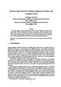
where Sm = set of competing routes with frequencies greater than or equal to Am; (Am – Am–1) = number of time windows containing only set of routes Sm in a 1-hr cycle; and min( f1, fk) = total number of time windows available to transfer passengers in a 1-hr cycle. To illustrate this formulation, consider an example with fk = 4 veh/hr and four competing routes R1, R2, R3, and R4 with frequencies f1 = 8, f2 = 4, f3 = 2, and f4 = 1 veh/hr. From the formulation, A1 = 1, A2 = 2, A3 = 4, min ( f1, fk) = 4, p1 = 0.25, p2 = 0.25, p3 = 0.5, S1 = {R1, R2, R3, R4}, S2 = {R1, R2, R3}, and S3 = {R1, R2}. As shown in Figure 1, in a 1-hr cycle, transfer passengers use a total of four time windows [min ( f1, fk) = 4]. S1, containing R1, R2, R3, and R4, is available in only one out of the four time windows (A1 = 1). S2, containing R1, R2, and R3, is available in two out of four time windows (A2 = 2). S3, containing R1 and R2, is available in all four time windows (A3 = 4). One out of the four time windows (A1 – A0 = 1 and p1 = 1/4 = 0.25) has only S1 as the set of available competing routes. One out of the four time windows (A2 – A1 = 1, and p2 = 1/4 = 0.25) has only S2 as the set of available competing routes. Two out of the four time windows (A3 – A2 = 2, and p3 = 2/4 = 0.5) have only S3 as the set of available competing routes.

26

Paper No. 971011

TRANSPORTATION RESEARCH RECORD 1571

window. Under such an assumption, the coordinated route assignment model is modified accommodate the following two cases: 1. If the missed connection competing route is the route with the least downstream travel cost, then such route’s share transit demand is reassigned to the route with the second least downstream travel cost. 2. If the missed connection competing route, Ri, is the only available route in its time window, then its lost demand is reassigned to the route with the least downstream travel cost in the next available time window. For such a case to occur, Ri must be the only competing route whose frequency fi is greater than or equal to fk. If fi ≥ fk, then the lost demand of Ri is absorbed back by Ri, since Ri is the only available route in the next time window. If fi = fk, and Sm contains only Ri, then the lost demand of Ri is redistributed to either Ri itself or the route in Sm–1 with the least downstream travel cost. (Sm and Sm–1 are defined as in the vehicle-availability rule). To redistribute the lost demand of Ri, the number of time windows, N, that contain only Ri and that are between two consecutive time windows containing only the set of routes Sm–1 need to be computed. N can be expressed as N=

FIGURE 1

Vehicle availability at a coordinated terminal.

If the coordinated operations terminal is a demand origin, where passengers do not arrive at the terminal by a coordinated route, then passengers are assumed to arrive at the terminal by a random process. Under this condition, a slight modification of the coordinated route assignment formulation is necessary. The number of time windows available to transit passengers is no longer bounded by min ( f1, fk) but by f1, the maximum frequency of all competing coordinated routes. As a result, f1 becomes the denominator in Equation 1 and F, the set of frequencies of all coordinated routes, contains only f1, f2, f3, . . . , and fn. After obtaining all possible sets of available competing routes (Sm), and the associated percentages ( pm) of the time windows containing only Sm, the least downstream travel cost rule is then applied to each Sm. The proportion of demand pmdij is assigned to the route in Sm with the least downstream travel cost.

Missed Connections of Coordinated Vehicles A further modification to the timed transfer assignment algorithm is necessary to account for the case of missed connections due to vehicles arriving behind schedule. Vehicles arriving at transfer terminals before their preset time windows have no effect on the trip assignment model. Therefore, the probability of the missed connection of interest is the probability of a coordinated vehicle arriving behind schedule. Unless the probabilities of missed connections of coordinated routes are considerably high, it is unnecessary to account for situations in which there is more than one missed coordinated route connection at transfer stations. In this model, it is assumed that at most one coordinated route may arrive behind schedule in each time

Am −1 fk

(2)

In only one of the N time windows is the lost demand of Ri caused by a missed connection distributed to the route in Sm–1 with the least downstream travel cost. Thus, a fraction of (1/N) of Ri’s demand is distributed to the route in Sm–1 with the least downstream travel cost, while the remaining fraction [(N−1)/N] of Ri’s demand is absorbed back by Ri. Let pmmc denote the probability of a missed connection of the route in Sm with the least downstream travel cost path. For each Sm, the following steps are a necessary modification to the trip assignment procedure: • Test: Check Sm to see if it contains only one route. If there is more than one route in Sm, proceed with Case 1’s modification. Otherwise, proceed with Case 2’s modification. • Case 1 modification: Assign pm(1 − pmmc) of the total trips to the route in Sm with the least downstream travel cost and assign pm pmmc of the total trips to the route in Sm with the second least downstream travel cost. • Case 2 modification: If f1 > fk, assign pm of the total trips to Ri. Otherwise ( fi = fk), assign [pm (1 − pmmc) + pm pmmc (N − 1)/N] of the total trips to the route in Sm with the least downstream travel cost and assign pm pmmc /N of the total trips to the route in Sm–1 with the least downstream travel cost.

TRIP ASSIGNMENT PROCEDURE FOR TIMED-TRANSFER SYSTEMS The trip assignment model presented here adopts the lexicographic strategy developed by Baaj and Mahmassani (9,10), which considers the number of transfers as the most important criterion. For those paths with the same least number of transfers, a “travel cost check” rule is employed to find the set of competitive paths. If one or more alternative paths pass the screen process, a frequency-share rule is applied. Since three types of terminal operations need to be considered in timed-transfer transit systems, various route assignment procedures are applied. The details of the timed-transfer transit trip assignment model are described hereafter.

Shih et al.

Paper No. 971011

0-Transfer Routes The trip assignment procedure for timed-transfer transit systems considers each demand pair separately. For a given demand pair (i, j), first of all, 0-transfer paths are searched for simply by checking the intersection of two sets of routes, SR0 and SRd, the sets of routes passing through origin i and destination j, respectively. If the intersection of SR0 and SRd is not an empty set, then the routes in the intersection set are classified as 0-transfer paths. Otherwise, it is not possible to assign the demand between i and j directly, and the set of 1-transfer paths needs to be identical. If there are 0-transfer paths, a travel cost check rule is applied to eliminate paths whose travel costs exceed the minimum travel cost path by a specified threshold. The travel cost for a 0-transfer path, TC0, is given by TC 0 = tinvtt , ij / R 0 + twait , i

(3)

where t invtt,ij /R0 equals the in-vehicle travel time from node i to node j using route R0, and twait,i is the waiting time at node i. If node i is a coordinated operations terminal, then the average waiting time is assumed to be half the preset time window. Otherwise, an average waiting time (in minutes) of (60.0/2f0) is applied. To obtain a more accurate estimation of average waiting times at a coordinated operations terminal, one may use the formulation developed by Lee and Schonfeld (11). Since the given demand dij can be assigned without transfer, route assignment will occur only at the origin node i. Thus, if node i is an uncoordinated operations terminal, the route assignment procedure for uncoordinated operations terminals should be applied. Otherwise, dij should be assigned according to the route assignment procedure for coordinated operations terminals, with TC0 taken as the downstream travel cost.

1-Transfer Routes If dij cannot be assigned directly, paths that connect i and j with one transfer are identified. The search process for 1-transfer paths is well documented by Baaj and Mahmassani (9,10). A 1-transfer path is represented by a list of the form [(R0, i, tnk) (Rd, tnk, j)]. For each path, passengers board route R0 at origin node at i, and stay on it until node tnk, where they transfer to route Rd, and travel on it until destination node j. The same travel cost check process described in the 0-transfer case is used to screen the set of competing paths, except that the travel cost for a 1-transfer, TC1, is now computed as TC1 = tinvtt ,i tnk / R 0 + tinvtt , tnk , j / R d + twait ,i + twait ,tnk + ttp

( 4)

where ttp is the penalty per transfer expressed in equivalent minutes of in-vehicle travel time. In the 1-transfer case, trips are not only assigned at the origin node, but also reallocated at the transfer node. At the origin node, trip assignment follows the same procedure as in the 0-transfer case, except that it is now applied to classes of paths rather than to individual paths. Paths that share the same starting route form one class of paths. According to the operation type at the origin node, demand is first allocated among alternative classes by the route assignment procedure. Within each class, demand is then totally assigned to the path with the least downstream travel cost among the constituent

27

paths (for the case of timed-transfer operation). The downstream cost for each path is the same as TC1. The downstream travel cost for each path class is the minimum downstream travel cost among all paths in that class. In addition, trips assigned to each path at the origin need to be reallocated at the transfer node. Paths with the same starting route (R0) and the same transfer node (tnk) form a group G0k. Based on the transfer node type, the total trips assigned to each group are redistributed to the paths in the group using the appropriate route assignment procedure. The downstream travel cost for each competing route at the transfer node is equal to {tinvtt , tnk , j / R d + twait , tnk + ttp}. 2-Transfer Routes If no 1-transfer paths can be found for dij, then 2-transfer paths are identified. The process of searching for 2-transfer paths is described in Baaj and Mahmassani (9). A possible 2-transfer path is represented by a list with three components, [(R 0, i, tnk)(Rc, tnk, tne) (Rd, tne, j)]. Such representation implies that passengers board route R0 at i, stay on it until node tnk, transfer to route Rc, travel on Rc until tn1, where they transfer to route Rd, and travel on it until destination j. If no 2-transfer paths can be found, dij is classified as unsatisfied demand, and the assignment procedure stops. The travel cost for a 2-transfer path, TC2, is computed as TC 2 = tinvtt , i , tnk / R 0 + tinvtt , tnk tn1 / R c + tinvtt , mtn1, j / R d + twait , i + twait , tnk + twait , tn1 + 2ttp

(5)

The trip assignment at the origin and at the first transfer node follows the same procedure as in the 1-transfer case, except that the downstream travel cost for a path at the origin is TC2 and at the first transfer node is (tinvtt, tnk tn1 /Rc + tinvtt, tn1,j /Rd + twait, tnk + twait, tn1 + 2ttp). Similarly, at the second transfer node, paths with the same upstream routes (R0 and Rc) and transfer nodes (tnk and tn1) form a group Gokcl. The downstream travel cost for each path at the second transfer node is computed by using (tinvtt, tn1,j /Rd + twait, tn1 + ttp). Applying the route assignment procedure relevant to the second transfer node type, the total demand of each group is reallocated to the paths within the group. NUMERICAL APPLICATIONS TO SINGLE DEMAND PAIR To demonstrate the timed-transfer assignment procedures, the authors apply it to the case of a single demand pair (i,j) served by seven routes, as shown in Figure 2. Four cases are considered: (a) an uncoordinated network, (b) a fully coordinated network with integer-ratio headways, (c) a fully coordinated network with a common headway, and (d) a fully coordinated network with integer-ratio headways and a missed connection probability p = 0.1 for all routes. Link travel times are given in Table 1. Case 1, 2, and 4 use the same route frequencies presented in Table 1. A 5-min time window is used in all the coordinated operation examples. The threshold for the travel cost check is set to be 10 percent. A 5-min penalty per transfer is assumed for all cases. No 0-transfer route can be found in the given route network. Six 1-transfer paths are found using the 1-transfer path searching process. The link components of each path are presented in Table 2. The path travel costs for uncoordinated and coordinated operations as well as the downstream travel cost at the transfer node for coordinated operations are given in Table 2. After the travel cost

FIGURE 2

TABLE 1

TABLE 2

Example route network with six one-transfer paths.

Link Travel Times (min) and Route Frequencies (Buses per Hour)

Path Links and Path Travel Cost

Shih et al.

Paper No. 971011

screening process is implemented, Paths P6 and P2 are eliminated from the set of 1-transfer paths in the uncoordinated and coordinated cases, respectively. Using the coordinated operation with integer-ratio headways as an illustrative example, five competing paths are divided into two path classes, C1 and C5, corresponding the Routes R1 and R5, respectively (the starting routes at the origin node i). Class C1 contains three paths, P1, P3, and P4 (Path P2 was eliminated earlier by the travel cost screening process). Class C5 contains two paths, P5 and P6. Demand dij is first assigned to the competing paths at the origin node i using the route assignment procedure for coordinated operation terminals. This procedure finds two sets of available competing routes S1 = {R1, R5} and S2 = {R1} with corresponding percentages of p1 = 0.5 and p2 = 0.5. In the time window containing S1, half of dij is assigned fully to C5, because C5 has the minimum travel cost, while in the time window containing S2, half of dij is assigned to C1 (R1 is the only route in S2). C1’s demand is assigned to P1, since P1 has the least downstream travel cost among all competing paths in C1. Similarly, C5’s demand is assigned to P5. Demand assigned to the competing paths at the origin is reallocated at the transfer nodes. Three path groups—G11 = {P1, P3}, G12 = {P4}, and G53 = {P5, P6}—are formed; each group contains the same starting route and transfer node. Using the route assignment procedure for coordinated operation terminals, the total demand of G11 (0.5dij) is reallocated to P1 and P3, and the total demand of G53 (0.5 dij) is reallocated to P5 and P6. In the final assignment, 0.5dij is assigned to P1,and 0.5dij is assigned to P5. This trip assignment procedure has been implemented in the LISP computer language whose “list” data structure representation is specially suited to handle the heavy path search and enumeration activities in the assignment logic (9,12). Table 3 gives the percentage of demand assigned to each path for each case. The percentage of dij assigned to each link is presented in Table 4. As expected, trip assignment in a fully coordinated system with a common headway is an extreme case. In this example, all demand is assigned to P5, the least travel cost path among the competing coordinated paths. In the uncoordinated system, demand tends to be assigned to competing paths with higher route frequencies, while in coordinated systems, demand tends to be assigned to competing paths with lower travel costs and higher route frequencies. Flow in coordinated systems is more concentrated than in uncoordinated

29

systems. In the missed connection example, only a small amount of demand (0.025dij) shifts from P1 to P3. Thus, unless the probability of missed connections is high, missed connections result in only slight change in the overall trip assignment.

CONCLUDING REMARKS In this paper, a trip assignment model for timed-transfer transit systems is presented. The model uses a lexicographic strategy with transfer avoidance or minimization as the main criterion and a travel cost check rule with a threshold value to define a set of competing routes. Trip assignment at transfer terminals follows rules that combine the concepts of vehicle availability and least travel cost. This leads to different assignment rules depending on the type of transfer terminal (uncoordinated versus coordinated operations). Preliminary results from numerical examples pertaining to one origin-destination pair may be summarized as follows: 1. In uncoordinated transit networks, trips tend to be assigned to competing paths with higher route frequencies. 2. In a fully coordinated transit network with a common route frequency, demand is completely assigned to the competing path with the minimum travel cost. 3. In coordinated transit networks, trips are more concentrated and tend to be assigned to paths with fewer travel costs and higher route frequencies. 4. Unless the probability of a missed connection is high, the overall trip assignment is not significantly changed. The timed-transfer trip assignment model is being implemented as part of AI-BUSNET, a comprehensive artificial intelligence– based bus network design tool that was developed at the University of Texas at Austin (9). AI-BUSNET is implemented in LISP, a fifthgeneration computer language whose “list” data structure is tailored toward the kind of computational activity taking place in transit network design—namely, path search and enumeration. The program now runs on an Apple MAC II computer equipped with a specialpurpose TI Explorer microchip that runs the LISP language compiler. The timed-transfer trip assignment model is the foundation of a currently developed analysis and evaluation model for timed-transfer

TABLE 3 Proportion of Demand Between Nodes i and j Assigned to Paths in All Cases

30

Paper No. 971011

TRANSPORTATION RESEARCH RECORD 1571

TABLE 4 Proportion of Demand Between Nodes i and j Assigned to Links in All Cases

transit systems. Using link flow information obtained from the timedtransfer trip assignment model, the analysis and evaluation model will be able to compute a variety of systemwide performance measures and the associated resource allocation requirements. This information will help transit planners improve existing timed-transfer transit networks or design new such networks.

REFERENCES 1. Speiss, H., and M. Florian. Optimal Strategies: A New Assignment Model for Transit Networks. Transportation Research B, Vol. 23B, No. 2, 1989, pp. 83–102. 2. Dial, R. B. Transit Pathfinder Algorithm. In Highway Research Record 205, HRB, National Research Council, Washington, D.C., 1967, pp. 67–85. 3. Rapp, M. H., P. Mattenberger, S. Piguet, and A. Robert-Grandpierre. Interactive Graphic System for Transit Route Optimization. In Transportation Research Record 1619, TRB, National Research Council, Washington, D.C., 1976, pp. 27–33. 4. Lampkin, W., and P. D. Saalmans. The Design of Routes, Service Frequencies and Schedules for a Municipal Bus Undertaking: A Case Study. Operations Research Quarterly, Vol. 18, 1967, pp. 375–397.

5. Mandle, C. E. Evaluation and Optimization of Urban Public Transportation Networks. Presented at the Third European Congress on Operations Research, Amsterdam, the Netherlands, 1979. 6. Hasselstrom, D. Public Transportation Planning: A Mathematical Programming Approach. Ph.D. thesis. Department of Business Administration, University of Gothenburg, Sweden, 1981. 7. Florian, M., and H. Speiss. On Two Mode Choice/Assignment Models. Transportation Science, Vol. 17, 1983, pp. 32–47. 8. Han, A. F., and N. H. M. Wilson. The Allocation of Buses in Heavily Utilized Networks with Overlapping Routes. Transportation Research B, Vol. 16B, No. 3, 1982, pp. 221–232. 9. Baaj, M. H., and H. S. Mahmassani. TRUST: A Lisp Program for the Analysis of Transit Route Configurations. In Transportation Research Record 1283, TRB, National Research Council, Washington, D.C., 1990, pp. 125–135. 10. Baaj, M. H., and H. S. Mahmassani. Hybrid Route Generation Heuristic Algorithm for the Design of Transit Networks. Transportation Research C, Vol. 3, No. 1, 1995, pp. 31–50. 11. Lee, K. K. T., and P. Schonfeld. Optimal Headways and Slack Times at Multiple-Route Timed-Transfer Terminals. Working Paper 92–22. Transportation Studies Center, University of Maryland, College Park, 1992. 12. Taylor, M. A. P. Knowledge-Based Systems for Transport Network Analysis: A Fifth Generation Perspective on Transport Network Problems. Department of Civil Engineering, Monash University, Victoria, Australia, 1989. Publication of this paper sponsored by Committee on Bus Transit Systems.