TS2-tree - an efficient similarity based organization for trajectory data. Petko Bakalov
Eamonn Keogh
Vassilis J. Tsotras
University of California, Riverside
University of California, Riverside
University of California, Riverside
[email protected]
[email protected]
ABSTRACT The increasingly popular GPS technology and the growing amount of trajectory data it generates create the need for developing applications that efficiently store and query trajectories of moving objects. In this paper we introduce TS2 tree, a novel indexing structure for organizing trajectory data based on similarity between trajectories. TS2 tree provides lower and upper bounds on distance between trajectories, based on which we propose a general framework for effectively answering a wide range of similarity-based trajectory queries such as similarity threshold (ST) query and similarity best fit (SBF) query. The multifold reduction in query computation times and the number of I/O operations is demonstrated through an extensive experimental evaluation.
Categories and Subject Descriptors H.3.1 [Indexing Methods]: Information Storage and Retrieval
General Terms Algorithms, Experimentation, Performance
Keywords Indexing, Similarity, Trajectory
1.
INTRODUCTION
With the high availability of GPS devices and advances in communications and sensor technology (RFIDs etc.), applications for monitoring and tracking moving objects have emerged. Such applications create large repositories of spatiotemporal data which are trajectorial in nature. Their large volume motivates the need to develop efficient techniques for managing and querying trajectories. One of the most popular trajectory query types focuses on finding similarities between trajectories. Here, the query typically specifies a trajectory and the answer contains all trajectories in the repository that are "similar" to the given trajectory. [6] [4]. Spatial similarity is measured through different distance metrics defined for trajectorial data (e.g Euclidean distance, Manhattan distance etc.) and is useful in many monitoring and surveillance applications. In this paper
[email protected]
we examine two variations of this problem, namely the similarity threshold (ST) and the similarity best fit (SBF) queries discussed below. Our focus is in developing a novel technique to index trajectories for answering the ST and SBF queries efficiently. Consider the scenario discussed in [4] where an urban planing tool is used to measure the benefits generated from adding extra bus lines to a public transportation system using a spatiotemporal archive. In this scenario a benefit is expressed as the number of commuter trajectories in the archive which are similar to the trajectory of the proposed bus line. Time is important, since a bus schedule should follow the proposed route at times when commuters are traveling it and thus will prefer to take the bus instead of their car. In this ST query example, the similarity between the bus route and a trajectory from the archive is defined by their spatial "closeness" expressed by a threshold ² (e.g. for example no further than 3 miles) around the bus route. The ST query returns the set of all trajectories which are completely covered by the 3 mile envelope crated around the proposed bus route. In contrast, a SBF query returns as a result the trajectory from the archive which is "the best fit" to the query trajectory. The evaluation of the above queries with existing spatiotemporal indexing techniques, which view a trajectory as a line in the n + 1 dimensional space is however computationally expensive and inefficient [3] [2]. A trajectory is typically decomposed in segments which are then approximated by Minimum Bounding Boxes (MBBs) and organized using a multidimensional index structure (R-tree). This approach however has various disadvantages: (i) The approximation of a line segment with a MBB introduces a large amount of "dead space" and as a result the discrimination capability of the index structure deteriorates. (ii) The index structure does not preserve a global picture of the trajectory. Instead, the trajectory segments can be scattered in different parts of the index structure. (iii) Traditional indexing techniques do not cluster trajectories according to their similarity. The above problems imply that a better indexing technique should maintain a global view over a trajectory and at the same time use a better trajectory approximation and perform clustering. In this paper we propose a novel indexing structure called Time-Specific Similarity Tree (TS2 Tree) with these properties which make the it a very efficient organization for evaluating time-specific similarity queries on trajectories.
2. PROBLEM DEFINITION Permission to make digital or hard copies of all or part of this work for personal or classroom use is granted without fee provided that copies are not made or distributed for profit or commercial advantage and that copies bear this notice and the full citation on the first page. To copy otherwise, to republish, to post on servers or to redistribute to lists, requires prior specific permission and/or a fee. Copyright 200X ACM X-XXXXX-XX-X/XX/XX ...$5.00.
For simplicity in the rest of the paper we assume that a moving object trajectory is defined as a sequence of location/time instant pairs. Other representations can be easily reduced to this general form by interpolation. More formally: Definition 1. A trajectory T i is a sequence of hlocation /timei pairs: {hl1 , t1 i, . . . , hln , tn i}, where li ∈ Rd , ti ∈ N
Here the location li is a d dimensional vector. With li .v we denote the v-ith component of this vector. For our 2-dimensional examples however we use the li .x and li .y to refer to the x and y coordinates. Assume that we are given trajectory distance function D. Having this function, a set of trajectories T ≡ {T 1, . . . , T k} and a query trajectory T q the Similarity Threshold (ST) query and the Similarity Best Fit (SBF) query are defined as follows:
t 4 3 Frames
2
(4,2)
1
(3,2)
Definition 2. Given D, T , T q and a spatial threshold ², a Similarity Threshold query returns the set of trajectories R ≡ {Ru, . . . , Rv} such that R ⊂ T and D(Ri, T q) ≤ ², ∀i where Ri ∈ R. Definition 3. Given D, T and T q, a Similarity Best Fit query returns trajectory Rj such that Rj ⊂ T and D(Rj, T q) ≤ D(T i, T q) , ∀i where T i ∈ T . In order to organize the trajectories in the repository for the purposes of efficient similarity search we need an approximate representation of the trajectories and a lower-bounding distance function defined over this representation. As is typical in similarity query processing, we employ a two step query evaluation strategy (for both ST and SBF queries). In the first phase we perform early pruning in the set of trajectories T using the approximate representation and the lower-bounding distance function. In the second step, the remaining small, approximate set of candidate trajectories is tested against the query trajectory Tq , this time using the raw trajectory data. For the purposes of trajectory similarity search we use the symbolic representation proposed in [1] for trajectories. This method utilizes the Piecewise Aggregate Approximation (PAA) [5] which was used to transform a time-series data into a string. The PAA algorithm accepts as input a trajectory of length n of hlocation /timei pairs and produces as output a trajectory approximation of reduced size, say m (m , . . . , < ln , tn > } of length n and a target length m ¿ n, PAA produces an approximate trajectory T¯i = {< ¯ l1 , t1 >, . . . , < ¯ lm , tm >} where the n n spatial values contained inside each time frame [ m (i−1), m i], 1 ≤ i ≤ m are replaced by their arithmetic mean: n
m ∀v ∈ [1; d] ¯ li .v = n
i m X
lj .v
n (i−1)+1 j= m
The approximation produced above is then discretized to a symbolic representation. For this purpose a uniform space grid is used where a unique label is associated to every discrete grid cell in the grid. The labels are assigned according to the grid cell position in the x and y axis starting with label (A,A) in the lower left corner of the grid. Each label has x and y components. By using the grid cell label instead of the average spatial location for each frame a trajectory is converted into a symbolic representation. A 2-dimensional example is shown in Figure 1. The symbolic representation can formally be defined as follows: Definition 5. Given a uniform grid with granularity τ assign an alphabet of symbols A = {α1 , . . . , αw } such that ∀1 ≤ j ≤ w : [τ (j − 1), τ j) → αj (every symbol is assigned to a unique interval of the grid). A trajectory Ti of length n can be approximated as a string T˜i = h˜ l1 · · · ˜ lm i of length m ¿ n, by replacing every value ¯ li .v in the m-length PAA approximation of Ti with symbol ¯ li .v = αj such that τ (j − 1) ≤ ¯ li .v < τ j.
(3,3)
X
(2,3)
Y
Figure 1: An object trajectory with its PAA representation; the string representation is: (2,3)(3,3)(3,2)(4,2). t 8 7 6 5 4 3 2 1 X
Y
Figure 2: Trajectory envelope Given a trajectory distance function D, for efficient pruning in ˜ in that the approximation space, we need a distance function D space, that lower-bounds D. Getting such symbolic distance function is simple for many trajectory distance functions (Euclidean, Manhattan etc.)
3. THE INDEX STRUCTURE We first describe the notion of an “envelope" which is used to cluster symbolic approximations among many similar trajectories. Then we discuss how envelopes can be combined hierarchically to create the TS2 tree.
3.1
Trajectory envelope
Until now we have taken each trajectory T i and first got its PAA approximation T¯i which was then turned into a symbolic representation T˜i. The next step is to provide an efficient representation for a set of similar trajectories. Assume for simplicity that all symbolic representations of trajectories have the same length m (the extension to cover trajectories with different lengths is straightforward). Consider a set of k trajectory symbolic representations T˜1 · · · T˜k. From this set we can derive two new sequences of grid labels U and L (each of length m) called respectively an upper and lower bound. The L sequence is derived by taking for each position from 1 to m the smallest x and smallest y label component on this position from all k strings. The U string is derived in a similar way taking for each position the largest x and y components. Ui .x = max(T 1i .x, .., T ki .x), Ui .y = max(T 1i .y, .., T ki .y)
Li .x = min(T 1i .x, .., T ki .x), Li .y = min(T 1i .y, .., T ki .y) An example is shown on figure 2 where we have three trajectories and their symbolic representations. The upper and the lower bound of the set of three sequences are: L = hD, DihD, DihC, EihB, F ihB, F ihB, F ihB, GihB, Hi U = hE, CihE, DihD, DihC, DihC, EihC, EihC, F ihC, Gi For the rest of the paper we use the term trajectory envelope to refer to the combination of U and L, and denote it as T E: T E ≡ (U, L) Sequences U and L form the smallest possible bounding envelope in the 3-dimensional space that encompasses this set’s symbolic representations T˜1 · · · T˜k from above and below. An important property of the trajectory envelope structure is that it can be used as an aggregation of the enclosed set of trajectory representations. Consider evaluating a threshold-epsilon query for a trajectory T q within a set of trajectories {T 1 · · · T k}. Assume that the symbolic representations of these trajectories have been computed and combined under a single trajectory envelope. Using the upper U and the lower L bounds of the envelope we can easily compute an upper and lower bound distance between the query trajectory T q and all trajectories in that envelope. If the lower bound distance is larger than threshold epsilon then we can safely prune all trajectories in this envelope. In the case of a best fit query, both the upper and lower bounds are utilized to direct the search. Another important property of trajectory envelopes is that they can be nested and thus combined in a hierarchical tree structure. This is due to the fact that a single trajectory representation is a special case of a trajectory envelope where both the upper and lower bounds are identical to the representation ( ∀i Li .x = T i.x = Ui .x ; Li .y = T i.y = Ui .y). We can thus combine a set of trajectory envelopes T E1, .., T Ek into a single one by finding maximum and minimum values for each position, from all envelopes. We use this property as the building block of the TS2-tree.
3.2
The TS2-tree
We utilize the nesting property of the trajectory envelopes to organize them hierarchically into a height balanced tree structure similar to an R-tree or B-tree. The tree structure partitions the spatiotemporal space with hierarchically nested, and possibly overlapping, trajectory envelopes. We refer to this structure as a TS2-tree. Similarly to the R-tree, the nodes in the TS2-tree contain a variable number of elements between some pre-defined minimum and maximum values. Each leaf node in the tree stores a trajectory symbolic representation as well as a pointer to the raw trajectory storage where we keep the actual trajectory data. Each entry within a non-leaf node stores a pointer to a child node, and the bounding envelope of all entries within this child node. The proposed structure is completely dynamic which means that the insert and delete operations can be intermixed with search ones. Insertions of trajectory symbolic representations in the tree are similar to the insertions in R-tree family. The algorithm examines the bounding trajectory envelopes in the non leaf nodes of the tree to find an envelope which overlaps with the new trajectory representation e.g. an envelope for which ∀i Li .x ≤ T i.x ≤ Ui .x ; Li .y ≤ T i.y ≤ Ui .y. If there is no such envelope the algorithm chooses the one which needs least enlargement to include the new trajectory representation. After choosing an appropriate envelope the algorithm continues recursively in the corresponding subtree. When the leaf level is reached and there is space available
Algorithm 1 Similarity best fit query Input: T q: document, R: TS2 root Output: The set of trajectories S which satisfy the query 1: Set B ← ∅; N ← R; U B = ∞; BF T ← ∅; BF D = ∞; 2: T˜q = CreateEnvelope(T q); 3: while N is not empty do . TS2 tree traversal 4: C = N .pop(); 5: for each child E of node C do 6: if E is a leaf then ˜ 7: if D(E.approximation, T˜q) < U B then 8: B.push(E); ˜ 9: UB = D(E.approximation, T˜q); 10: else ˜ 11: if D(E.lower, T˜q) < U B then 12: N .push(E); ˜ 13: if D(E.upper, T˜q) < U B then ˜ 14: UB = D(E.upper, T˜q); 15: end for; 16: end while; 17: while B is not empty do . Verification step ˜ = B.pop(); 18: B ˜ 19: B = RawStorageLookUp(B); 20: if D(B, T q) < BF D then ˜ 21: BF T ← B.id; 22: BF D = D(B, T q); 23: end while;
in the current node the new trajectory representation is simply inserted there. Otherwise the leaf node is split. For the splits we adopt the R*-tree approach to determine the distribution of the envelopes between the nodes which minimizes the overlapping between the trajectory envelopes. The intuition behind this approach is that the probability for two envelopes to satisfy simultaneously the search criteria is proportional to their overlapping area. The process of splitting nodes is propagated up to the root of the tree if it is necessary.
4.
QUERY EVALUATION
In this section we will discuss the evaluation algorithms for both queries: (i) Similarity threshold (ST), and, (ii) Similarity best fit (SBF).
4.1
Similarity threshold query
The input to the Similarity threshold algorithm is the root of the TS2 tree, the query trajectory T q and the spatial threshold ². The algorithm traverses the index tree from the root to the leaf nodes in a top down manner. At each step, the algorithm checks the bounding envelopes at the current node: if there is overlapping between a bounding envelope and the the envelope produced by expansion the query trajectory T q with ² in each spatial dimension for each time instance, the algorithm is executed recursively for the corresponding subtree. Similarly to R-tree, due to the overlapping envelops, the algorithm may need to visit more than one subtree under the current node. After the traversal of the tree we have a verification step where we examine the content of the candidate set generated in the previous step. We load the raw trajectory data for each candidate trajectory and compare it with the query trajectory T q. If the candidate trajectory satisfies this verification we place it in the result set.
4.2
Similarity best fit query
The input to the Similarity best fit algorithm is the root of the TS2 tree and the query trajectory. As in the Similarity threshold query the best fit algorithm traverses the index tree from the root to the
EXPERIMENTAL EVALUATION
We proceed with the experimental evaluation of the proposed techniques. In our experiments we use synthetic data. The queries are based on actual trajectories slightly skewed in the time and space from the original. We compare the performance of the proposed TS2 tree with the MVR tree approach proposed by [2] using two measures: The average number of index node accesses and the average number of data pages per query that need to be retrieved from storage for verification of the result.
5.1.3
Varying the length of the trajectory MVR-tree
2500
600
2000 1500 1000 500
ST MVR-tree
ST TS2 tree
SBF TS2 tree
SBF MVR-tree
SBF TS2 tree
1400 1200 1000
Data Pages
Node Access
ST TS2 tree
SBF MVR-tree
1000 800 600 400 200
800 600 400 200
0
0 100
250
500
100
250
Dataset size
500
Dataset size
Figure 3: Perf. vs. Size In the first group of experiments we measure the performance for different data set sizes. The results are shown in figure 3. As it can be depicted from the plots when the dataset size (in thousands) increases, the numbers of data pages and index nodes accessed are also growing. For the ST query the number of index nodes and the raw trajectory data pages accessed by the TS2 tree is lower than the corresponding number for the MVR tree for all three datasets. The improved approximation in TS2 tree requires checking fewer index nodes and generates fewer candidates. For the SBF queries both index structures converge fast on a small candidate set. This is because the queries are not random but relevant to the trajectories. Pruning is fast because both algorithm use variations of best first search.
Varying the Spatial threshold ²
5.1.2
TS2 tree
1400
1200
1200
1000
1000
Data Pages
Node Access
MVR-tree 1400
800 600 400 200
MVR-tree
TS2 tree
20
30
800 600 400 200
0
0 10
20
30 Threshold
40
400 300 200
0 100
150
50
100
150
Time period
Figure 5: Perf. vs. Time
ST MVR-tree
1200
500
Time period
Varying the Dataset Size
1400
TS2 tree
100
0
Experimental Results
5.1.1
MVR-tree 700
50
5.1
TS2 tree
3000
Data Pages
5.
that by increasing the spatial threshold ² the query becomes more relaxed and thus more expensive for evaluation. We use four different values for ² varying from 10 to 40 miles. The results are shown in figure 4. As expected with the increase of the threshold parameter the number of index nodes and the raw trajectory data pages accessed by both: the TS2 tree and the MVR tree increases. However the TS2 tree index node access increase has a slower rate when compared to the MVR tree increase due to the holistic approach (e.g using envelopes that approximate the whole trajectory than MBRs which approximate only trajectory segments) in the tree traversal.
Node Access
leaf nodes keeping the smallest upper bound distance U B between a query and envelope discovered so far. At each step, the algorithm checks the lower bound distance of the bounding envelopes at the current node and the query trajectory T q. If the distance is smaller than the U B the algorithm is executed recursively for the corresponding subtree. If it is not this means that we already have a better candidate and we can prune this part of the tree. At the end we have a verification step (lines 17-23) where we find the best fit trajectory from the reduced candidate set using raw trajectory data.
10
40
Threshold
Figure 4: Perf. vs. Spatial threshold In the next set of experiments we test the behavior of the similarity threshold (ST query) algorithm for increasing values of the query threshold ². The intuition behind this set of experiments is
In the last group of experiments we tested the behavior of the proposed indexing structure and algorithms for different values of the trajectory length varying from 50 up to 150 minutes. The results are shown in figure 5. As it can be observed increasing the length of the trajectories the performance of the TS2 tree deteriorates. This is due to the fact that longer trajectories are more likely to be dissimilar which will deteriorate the clustering in the TS2 tree. The trajectory envelopes become wider which also increases the overlap between the different nodes. An interesting observation is that the number of raw data I/Os decrease for the MVR tree decreases. This is due to the fact that by increasing the length of the query it becomes more restrictive.
6.
REFERENCES
[1] P. Bakalov, M. Hadjieleftheriou, E. Keogh, and V.J. Tsotras. Efficient trajectory joins using symbolic representations. In Proc. of the International Conference on Mobile Data Management (MDM), 2005. [2] M. Hadjieleftheriou, G. Kollios, V. J. Tsotras, and D. Gunopulos. Efficient indexing of spatiotemporal objects. In Proc. of Extending Database Technology (EDBT), pages 251–268, 2002. [3] G. Kollios, V.J. Tsotras, D. Gunopulos, A. Delis, and M. Hadjieleftheriou. Indexing animated objects using spatiotemporal access methods. IEEE Transactions on Knowledge and Data Engineering (TKDE), 13(5):758–777, 2001. [4] B. Lin and J. Su. Shapes based trajectory queries for moving objects. In GIS ’05: Proceedings of the 13th annual ACM international workshop on Geographic information systems, pages 21–30, 2005. [5] J. Lin, E. Keogh, S. Lonardi, and B. Chiu. A symbolic representation of time series, with implications for streaming algorithms. In Proc. of ACM SIGMOD workshop on research issues in data mining and knowledge discovery, pages 2–11, 2003. [6] Yutaka Yanagisawa, Jun ichi Akahani, and Tetsuji Satoh. Shape-based similarity query for trajectory of mobile objects. In MDM ’03: Proceedings of the 4th International Conference on Mobile Data Management, pages 63–77, 2003.