TSpec: A Notation for Describing Memory Reference Traces University of Virginia Department of Computer Science Technical Report CS-2000-23 August 14, 2000 †Dee
A. B. Weikle, †Kevin Skadron, *Sally A. McKee, †William A. Wulf †Department
of Computer Science University of Virginia, 151 Engineer's Way, PO Box 400740 Charlottesville, VA 22904-4740 {daw4q |
[email protected],
[email protected]} *Department
of Computer Science University of Utah 50 S. Central Campus Dr., #3190 Salt Lake City, UT 84112-9205 {
[email protected]}
Abstract Interpreting reference patterns in the output of a processor is complicated by the lack of a succinct notation for humans to use when communicating about them. Since an actual trace is simply an incredibly long list of numbers, it is difficult to see the underlying patterns inherent in it. The source code, while simpler to look at, does not include the effects of compiler optimizations such as loop unrolling, and so can be misleading as to the actual references and order seen by the memory system. To simplify communication of traces between researchers and to understand them more completely, we have developed a notation for representing them that is easy for humans to read, write, and analyze. We call this notation TSpec, for trace specification notation. It has been designed for use in cache design with four goals in mind. First, it is intended to assist in communication between people, especially with respect to understanding the patterns inherent in memory reference traces. Second, it is the object on which the cache filter model operates. Specifically, the trace and state of the cache are represented in TSpec, these are then the inputs for a function that models the cache, and the result of that function is a modified trace and state that are also represented in TSpec. Third, it supports the future creation of a machine readable version that could be used to generate traces to drive simulators, or for use in tools (such as translators from assembly language to TSpec). Finally, it can be used to represent different levels of abstraction in benchmark analysis. 1. Introduction The work of today’s cache designer is becoming increasingly difficult. It is well-accepted that there is a processor-memory performance gap that must be compensated for with the caching system. [Bur95, Hen96, Jou97, Wul94] Every time there is an increase in the speed of a microprocessor, the cache and corresponding memory system must be redesigned to feed the increased need 1
for instructions and data to operate on. There continues to be a constant level of research and improvement to cache functionality, but such research typically focuses more on improvements to the cache system itself and less on the process, or underlying theory behind cache design. The most common approach is to modify the cache hierarchy and then simply judge that design by running benchmarks through a simulator to determine hit rates or average memory access times. While it has yielded many improvements to the performance of caching systems, this approach is primarily ad-hoc experimentation with little unifying theory to guide new designs. This hampers the ability of the cache designer to effectively design to specific performance points, or fully understand the impact of research results on actual systems. For example, the interaction between specific features such as out-of order execution, branch prediction, pre-fetching, or cache replacement algorithms, in the real-time execution of a user application is unclear. Optimizing each one separately will not necessarily lead to a global optimum. In addition, it is difficult to control all the parameters one needs to perform an experiment that would answer this question. A final complicating factor is that the current approach to cache design depends on benchmarks and a simulation infrastructure that are non-standard and were developed primarily for the purpose of evaluating processor architectures. These simulators are extremely useful and appropriate for the specific area they were designed to explore, but do not provide a unified or complete experimental infrastructure. An analysis framework that allows researchers to abstract away from a particular environment to communicate ideas about the fundamental characteristics of memory systems would be beneficial. An integral part of this framework would be the ability to understand reference patterns of different processors for different source programs. Interpreting reference patterns in the output of a processor is complicated by the lack of a succinct notation for humans to use when communicating about them. Since an actual trace is simply an incredibly long list of numbers, it is difficult to see the underlying patterns inherent in it. The source code, while simpler to look at, does not include the effects of compiler optimizations such as loop unrolling, and so can be misleading as to the actual references and order seen by the memory system. To simplify communication of traces between researchers and to understand them more completely, we have developed a notation for representing them that is easy for humans to read, write, and analyze. We call this notation TSpec, for trace specification notation. It has been designed for use in cache design with four goals in mind. First, it is intended to assist in commu2
nication between people, especially with respect to understanding the patterns inherent in memory reference traces. Second, it is the object on which the cache filter model operates. Specifically, the trace and state of the cache are represented in TSpec, these are then the inputs for a function that models the cache, and the result of that function is a modified trace and state that are also represented in TSpec. Third, it supports the future creation of a machine readable version that could be used to generate traces to drive simulators, or for use in tools (such as translators from assembly language to TSpec). Finally, it can be used to represent different levels of abstraction in benchmark analysis. Our work focusses on four different levels of abstraction. Current cache analysis is based on single traces, so TSpec can specify an individual trace. However, there are many accidents of address binding by the compiler or loader in such a trace. It is desirable to be able to analyze all the traces that differ only in those artifacts of binding, or as we describe it, the equivalence class of traces that differ only because of those binding artifacts. So TSpec has been designed to describe the abstraction of an equivalence class under varying address bindings. Similarly, there are many traces that result from the execution of a single program which, given different input data, follows different execution paths through the program. Here again, we want TSpec to be able to represent such a level of abstraction. Finally, there exists a set of traces that result from both different address bindings and different input data. The following sections describe the TSpec constructs that are used to describe a single trace, where all the address bindings, and the path through the program are known. Descriptions of the other levels of abstraction and the TSpec constructs to support them begin in Section 4. 2. TSpec Constructs for Single Traces A trace specification is a formal rule that describes a specific trace. It consists of a set of definitions followed by a trace list. Definitions can be either variable or subtrace definitions. A trace list is a concatenation of trace atoms, the most basic TSpec construct, surrounded by angle brackets (). Trace atoms are concatenated by separating each trace atom with a comma (100, 200, 300). The simplest example of a trace specification has no definitions and only one trace in the trace list. It is a list of address references such as: 3
A trace atom may be (1) a literal, (2) the symbol λ, (3) a variable, or (4) a subtrace. A literal is a an integer with an optional attribute tag. The integer represents an address, and may be specified in decimal or hexadecimal; hexadecimal numbers will be preceded by 0x. The attribute tags are not defined by TSpec, but are intended to connote code vs. data, read vs. write, system vs. user, etc. For the purpose of this document, non-null attribute tags will be represented by an underscore and one or more letters appended to the end of an integer representing the address — thus 100_cr is an integer/tag pair. λ is used as a placeholder for an integer/tag pair. Its primary role is in the merging of multiple traces and will be described in more detail later. Variables and subtraces are constructs that allow regular patterns of literals to be described compactly. They are described more fully in Section 2.1, Section 3.1 and Section 2.4 respectively. 2.1 Simple Variables and Operations on Variables More will be said about variables later, but here we introduce the basic concept and the simple operations on them. A variable represents a regular sequence of addresses and is specified by a base address and an increment or decrement (stride). An example of a variable definition is x(400,8). x is the name of the variable, 400 is the value of the base address and 8 is the value of the increment. A variable can be initialized (denoted #x) to set its current value to its base address. A variable can also be post-incremented (denoted x+) to add the increment to its current value or post-decremented (denoted x-) to subtract the increment from its current value. Each time a variable occurs, it generates an address. Note that the + and - operators are subscripts. The reason for this will be seen later. 2.2 Definite Iteration A list of trace atoms can be grouped together with parentheses and an optional label. In this way the group is set apart to assist in pattern identification, or to be operated on. The format of a parenthesized group is (100, 200, 300) or (LABEL 100, 200, 300)LABEL. A trace atom or a group of trace atoms can be repeated with the iteration operator, *. For example, x*4 repeats the value represented by x, 4 times. (Lx+)L*4 generates the value of x and postincrements x four times. If the initial value of x was 100 and the increment 4, the above would generate the address list (100, 104, 108, 112) and the next time x was used, it would generate the address 116.
4
2.3 Suppression Operator To suppress the generation of a construct’s address while operating on that construct, any of the above operations can be preceded by !. For example, !#x would initialize the variable x to its initial value where #x would initialize the variable x to its inital value and generate that value. 2.4 Subtraces Often it is useful to separate out a part of a trace that is reused frequently and use a label to refer to it rather than specifying the whole trace. This makes larger patterns in the reference stream more obvious. It is also useful to have parameters for these subtraces in the instances where subtraces are the same except for one or two positions. The definition of a subtrace has the form: s(p1, p2) = The name of the subtrace is s. p1 and p2 are parameters to the subtrace and following the = symbol is simply another trace specification. When using the subtrace in a trace, the % operator indicates the subtrace should be “run” to completion (i.e. substituted as a whole into the trace). The specification s(p1, p2) = < %s(200, 300), %s(204, 304)> would generate the following trace:
The parameters of the subtrace are substituted textually, and then evaluated when that element of the subtrace is executed. This allows variables to be used as parameters; these variables are then evaluated in the context where they are substituted, and thus can evaluate to different addresses. For example, the above trace could also be generated by the following trace specification: s(p1, p2) = ; f(200; 4); t(300; 4); < !#f, !#t, %s(f+, t+), %s(f+, t+)> There are two modes of execution for a subtrace. The first is to run the subtrace from beginning to end without any intervening references. This is the mode demonstrated in both of the previous examples, is called running the subtrace, and is denoted with a % symbol preceding the name of 5
the subtrace (%s(f+, t+)). The second mode of address generation for a subtrace is called pulsing a subtrace and is denoted with an @ symbol before the name of the subtrace (@s(p1, p2)). Each subtrace has a control pointer which operates like the control pointer of a program. When a subtrace is “run”, the control pointer moves from the beginning to the end of the subtrace as each element is executed. When a subtrace is pulsed, the control pointer is moved one element and only the address(es) associated with that element are generated. The next time the subtrace is pulsed, the control pointer is moved one more element, and so on. To set the control pointer of a subtrace to the beginning the subtrace may be initialized with #, just like a variable. To suppress generation of addresses during initialization, ! should be used. d = ; c(100; 4); < !#d, (!#c, c+, @d, c+, @d, c+)*2> The above specification generates the trace below.
If a subtrace name is used without an @ or %, the element of the subtrace the control pointer is at is generated and the control pointer stays where it is. This is similar to a pulse without the update of the control pointer and is analagous to using a variable without an operator. 2.5 Merge The merge (denoted t1 & t2) of multiple traces is formed one “address” (or variable) at a time. The merge of a single address with any number of λs is defined to be the address. The merge of any number of λs is defined to be λ. The merge of more than one address is undefined. For example, < a1, λ, a3, λ> & < λ, a2, λ, a3> = < a1, a2, a3, a4>. It is easiest to visualize this operation by lining the traces up one above the other as if they were going to be “added” and merging each set in the same position in the reference string. & ------------------- Figure 3: Merge Example
6
3. Specific Examples So far we have discussed the basic element of TSpec (the trace atom), how a variable can represent a trace atom, and several operations including: - definite iteration of a variable or a trace(*), - initialization of a variable or a subtrace(#), - variable post-increment or decrement (+,-), - merge of multiple traces (&), and - concatenation of variables to form a trace (,).
Figure 1 shows a more complete example for a simplified version of the inner loop of a routine to copy a vector from one location to the another. The code in this example has been simplified to allow the pattern to be easily seen in the reference string. One might think of the first c+ as the load of the element being copied, the second as the store to the new location, and the third as the branch back for the next element. Notice that this TSpec description represents a very specific trace T, as the address bindings and the specific path through the program (number of iterations in this example) are known. C Code: TSpec:
for i=1 to 3 t[i] = f[i]; c(100; 4); f(200; 4); t(300; 4);
Reference String:
100, 200, 104, 300, 108, 100, 204, 104, 304, 108, 100, 208, 104, 308, 108
Figure 1: Copy example
3.1 Trace Variables In More Detail Now we can create a more complex example by introducing a more general definition and use of trace variables. Variables and the increment operator as introduced in Section 2.1 are adequate for describing any trace, but they are most convenient for 1-dimensional arrays. We shall therefore extend the definition and increment/decrement syntax to more naturally handle n-dimensional arrays, by using an arbitrary number of iterator value-count pairs instead of a single iterator. Consider the variable definition x(100; 4, 0; 64, 0) where x is the name of the variable, 100 is the base address (or starting address of the structure being accessed) and 4 and 64 are iterator values that can be added or subtracted from the value of the variable. The zeros are the base values of the 7
iterator counts. At any point in time the value of a variable is determined by the following formula: var = base + (ic1*iv1) + (ic2*iv2) + ... where var = the current value of the variable, base = the base address of the variable in the definition, ic represents the iterator count for a specific iterator, and iv represents the iterator value for a specific iterator. Incrementing an iterator count increases the value of the variable by the value of the iterator in the definition. Note that if only one value is present for an iterator, it is assumed to be the value of the iterator, and the iterator count is assumed to be zero. Generally speaking multiple increments are used to traverse a data structure such as a matrix with different strides and the number often reflects the number of loop nests used to traverse the structure. There are four operators that can be used to change the value of the iterator count(s). # initializes the value to its base value in the definition. + post increments the iterator count by 1, - post decrements the iterator count by 1, and ~ leaves it alone. The operators for the iterator counts appear as subscripts to the variable name in a trace. The iterator count operators appear as a comma separated subscript, called the control tag string. The position of the operator in the control tag string indicates which iterator will be used to increment or decrement the variable. The control character in the first position describes what will happen with the first iterator, the one in the second position what will happen with the second iterator, etc. Current convention is that the iterator that changes fastest is closest to the variable. As an example of this usage, consider the data portion of matrix multiplication, x * y = z: x(1000; 0,4; 0,N), y(4000; 0,4; 0, N), z(8000; 0,4; 0,N); Here the innermost loop does a read of a row from x and a read of a column from y, multiplying them and keeping a running sum of the products in z. z is traversed completely once. Each element of z is computed completely before going on to the next one. y is traversed by “column” (the second iterator first) while x is traversed by “row” (the first iterator first). 8
The following sections provide a more complete description of equivalence classes and the more advanced TSpec constructs to support them. At the end is a complete grammar for the TSpec notation. 4. Equivalence Classes In Depth and the Larger Picture As described above computer architects typically evaluate cache designs on a few specific traces. These traces are generated by running a particular benchmark suite on a simulation of their new design. This trace is then compared to another single trace resulting from a system that is as close as possible to the same, but without the particular improvement under investigation. While there has been significant work and improvements to benchmarks in the last decade, these results are still point solutions for a whole range of possible results for a specific piece of source code. For example, the results from benchmark runs are for one set of input data, one set of address bindings, and one compiler. Another instance of any of these parameters may produce drastically different results. To make it clear where a trace has come from and what type of dynamic run it corresponds to, we have developed the concept of equivalence classes of reference traces, or different levels of abstraction as described in the introduction. If two traces are in the same equivalence class, then they use the same piece of source code but may vary one or more parameters that are used to describe the equivalence class. For our work we have broken down the set of traces that could be generated by a specific piece of source code into four sets, depending on whether or not the address bindings are known and whether or not the input data is known. The relationship between these groups is shown in Figure 2. The specific trace generated by a benchmark could be thought of as the trace T. The set of traces that would be generated with the same source code and the same set of bindings as T, but with different sets of input data is denoted {Td}, and is referred to as the equivalence class of traces with respect to input data. {Tb} is referred to as the equivalence class of traces with respect to address bindings, and is the set of traces that has the same source code and input data as T, but a different set of address bindings. (Note that this is a generalization of the concept of translation arrays in [Har99].) {Tbd} is the set of traces that has the same source code, but varies the address bindings and the input data. Other equivalence classes exist, such as the equivalence class of traces under
9
varying virtual to physical address bindings, but we do not treat them in our work.1
Same bindings
Same data
Y N
Y
N
T
{Td}
{Tbd}
{Tb}
{Td}
{Tb} {Tbd} T
Figure 2: Equivalence Classes: The relationship between traces generated by a specific source program by varying bindings only ({Tb}), input data only ({Td}), or both bindings and input data ({Tbd}).
Each of the four sets shown in Figure 2 has corresponding constructs in TSpec. A specific trace, T, can be fully described using the constructs shown in Section 2 above. The set of traces {Tb}, the equivalence class of traces under varying address bindings, can be represented by the constructs described in Section 2, but without the base addresses. Consider the copy example in Figure 1. By substituting constant names for the specific base address information, one specification can describe a whole class of traces that includes all possible mappings of the code (variable c), and the two data streams (f and t). c(CSTART, 4); f(FSTART, 4); t(TSTART, 4);
Depending on the cache designer’s goal, this form of TSpec can be used to do a case analysis of what different mappings would mean to cache performance, or to allow the cache designer to abstract away from those side effects, choose a representative trace for the class as a whole, and understand how a particular cache system would handle the basic reference pattern. 5. Expanding TSpec to Describe {Td} and {Tbd} To describe the equivalence class of traces under varying input data, a way to express conditionals is required. Specifically, support for trace patterns generated by procedural case statements (if-
1. While examining kernels it is unlikely that a difference would appear between virtual and physical addresses. The actual addresses may differ, but the form of the reference pattern would be the same unless a page boundary was crossed or two virtual addresses mapped to the same physical page. In our work we always use virtual addresses. 10
then-else) or indefinite iteration of loops is needed. 5.1 Case Statements An if-then-else clause is a special case of a procedural case statement. To support the description of several different execution paths through a case statement, we use a parenthesized group of trace items separated by |. This denotes a set of smaller traces; only one of which is executed. For example: c(1000; 4); d(1020; 4); would generate one of the following two trace lists. or The above example describes a code segment where the last statement executed is an if-then-else. The then clause is represented by executing the last c+, and the else clause by d. Here, either the c+, or the d is executed, but not both. For clarity, it is sometimes desirable to label the conditional symbols (|) and the curly brackets that designate the set of possible statements so that their relationship is obvious. Labels are similar to those for parentheses. For example: c(1000; 4); d(1020; 4); There are times when the exact addresses being generated for the code of a case statement may not be important. In this situation, the same variable can be used in all possible cases and the form of the code loop is still clear. For example, the above pattern could be written as: c(1000; 4); d(1020; 4); 5.2 Indefinite Iteration and Break To represent indefinite iteration, the * symbol is used for loops without a corresponding number to represent the number of iterations. For example, x* means zero or more repetitions of x. The break construct is analagous to the break in C and continues the specification after the right parenthesis with the same label as the break. For example, consider the above example with a loop and break added. 11
c(1000; 4); d(1020; 4); Here, if the second case option is taken, the outer loop labeled R is exited. and execution continues with the last c+. These three constructs; case options (|), indefinite iteration (*), and break allow us to model very general paths through a piece of source code. 6. Notational Conventions The above paragraphs outline the formal notation. Often it is useful to have some shorthand for specific operations. The frequently used abbreviations are: - #x is used for #x#,#,.... This initializes the variable to its base address and all the increments to their initial value. - x+ is used for x+,~,~,... . The companion, x-, is also acceptable. - x* is used when the exact number of iterations is unimportant to the discussion. - Commas as a delimiter between trace atoms may be left out if the result is a description that is easier to read. - The label for a parenthesized group of trace atoms may be left out. - If only one number is present for a variable’s iterator, it is assumed to be the value of the iterator and the iterator count is assumed to be zero. - Sometimes the exact address and/or increment is unimportant to the discussion and trace lists will be used without their definition. For example, < (!#x, x+*)* > to demonstrate the form of the code references for a loop of indeterminate length, location, and number of iterations. 7. Grammar In this section, we provide the syntactic definition of the notation. Here, single quotes surround the delimiters of the language being defined. Thus, in the first definition below, a consists of a comma-separated sequence of s followed by a . ::= {‘,’}* {} ::= {‘&’}*’’ ::= {’,’}* | {’,’}* ::= ‘(‘ ‘;’ ‘)’ ::= ‘(‘ ‘)’ ‘=’ 12
::= {’;’}* ::= ’,’ ::= { ‘,’}* ::= ::= ‘(‘ ‘)’ ::= | ‘,’ ::= ‘!’ | ‘#’ | ‘!#’ | ‘(‘’)’ | ‘(‘ ‘&’ ‘)’ | ’*’ | | ‘break’ | ‘{‘ ‘|’ ‘}’ ::= | ‘λ’ | ::= | ::= { ‘,’ }* ::= ‘+’ | ‘-’ | ‘#’ | ‘~’
8. Related Work Other languages to describe memory reference traces are unknown to the authors. Previous work on TSpec, including a description of Tint, a TSpec interpreter that turns TSpec into an address trace is described in [McK97]. A general description of the overall framework that uses TSpec, including a description of the cache as filter concept, is included in [Wei98], [Wei00a], and [Wei00b]. 9. References [Bur95] D.C. Burger, J.R. Goodman, and A. Kagi, “The Declining Effectiveness of Dynamic Caching for GeneralPurpose Microprocessors”, Univ. of Wisconsin-Madison Computer Science Dept. Technical Report 1261, January 1995. [Har99] J. Harper, D. Kerbyson, and G. Nudd, “Analytical Modeling of Set-Associative Cache Behavior”, IEEE Transactions on Computers, vol. 48 no. 10, Oct. 1999.
[Hen96] John L. Hennessy and David A. Patterson. “Computer Architecture: A Quantitative Approach”. Morgan Kaufmann, second edition, 1996. [Jou97] N. P. Jouppi and P. Ranganathan, “The Relative Importance of Memory Latency, Bandwidth, and Branch Limits to Performance” ISCA 97 Workshop on Mixing Logic and DRAM: Chips that Compute and Remember June 13
1st, 1997, 8:30am-5:30pm Denver, Colorado. [McK97]S.A. McKee, Wm.A. Wulf, D.A.B. Weikle, “TSpec: A Specification Language for Reference Traces”, Univ. of Virginia Dept. of Computer Science Technical Report CS-97-19, August 1997. [Wei98] Dee A. B. Weikle, Sally A. McKee, Wm. A. Wulf, "Caches As Filters: A New Approach to Cache Analysis", Sixth International Symposium on Modeling, Analysis, and Simulation of Computer and Telecommunication Systems (MASCOTS'98), July19-24, 1998, Montreal Canada. [Wei00a]Dee A. B. Weikle, Kevin Skadron, Sally A. McKee, Wm. A. Wulf, “Caches As Filters: A Unifying Model for Memory Hierarchy Analysis”, University of Virginia, Computer Science Department, Technical Report, CS-200016, June, 2000. [Wei00b]Dee A. B. Weikle, Sally A. McKee, Kevin Skadron, Wm. A. Wulf, “Caches As Filters: A Framework for the Analysis of Caching Systems”, to appear in Grace Murray Hopper Conference 2000, Sept. 14-16, 2000. [Wul94] W. A. Wulf, and S. A. McKee, “Hitting the Memory Wall: Implications of the Obvious”, ACM Computer Architecture News. Vol. 23, No. 4, September 1995.
14