Tutorial Geometric Computing in Computer Graphics using ... - Gaalop

Dietmar Hildenbrand / Geometric Computing in Computer Graphics

Tutorial Geometric Computing in Computer Graphics using Conformal Geometric Algebra Dietmar Hildenbrand Interactive Graphics Systems Group, TU Darmstadt, Germany

Abstract Early in the development of Computer Graphics it was realized that projective geometry was well suited for the representation of transformations. Now, it seems that another change of paradigm is lying ahead of us based on Geometric Computing using Conformal Geometric Algebra. Due to its geometric intuitiveness, elegance and simplicity, the underlying Conformal Geometric Algebra appears to be a promising mathematical tool for Computer Graphics and Animations. In this tutorial paper we introduce into the basics of the Conformal Geometric Algebra and show its advantages based on two Computer Graphics applications. First, we will present an algorithm for the Inverse Kinematics of a robot that you are able to comprehend without prior knowledge of Geometric Algebra. We expect that here you will obtain the basic knowledge for developing your own algorithm afterwards. Second, we will show how easy it is in Conformal Geometric Algebra, to fit the best suitable object in a set of points , whether it is a plane or a sphere.

1

2


1. Introduction In this tutorial paper, we focus on the introduction of the 5D Conformal Geometric Algebra which is an extension of the 4D Projective Geometric Algebra. While points and vectors are normally used as basic geometric entities, in Conformal Geometric Algebra we have a wider variety of basic objects. For example, spheres and

Table 1: list of the conformal geometric entities

entity

representation 1

representation 2

Point

P = x + 12 x2 e∞ + e0

Sphere

s = P − 12 r2 e∞

s ∗ = x1 ∧ x2 ∧ x3 ∧ x4

Plane

π = n + de∞

π∗ = x 1 ∧ x 2 ∧ x 3 ∧ e ∞

Circle

z = s1 ∧ s2

z ∗ = x1 ∧ x2 ∧ x3

Line

l = π1 ∧ π2

l ∗ = x1 ∧ x2 ∧ e∞

Point Pair

Pp = s1 ∧ s2 ∧ s3

Pp∗ = x1 ∧ x2

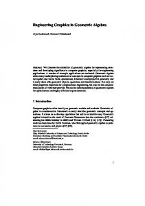
3. The outer product and the basic geometric entities in Conformal Geometric Algebra Figure 1: Intersection of two spheres

Table 1 lists the two representations of the geometric entities in Conformal Geometric Algebra. Please find details in [8] and [11].

circles are simply represented by algebraic objects. To represent a circle you only have to intersect two spheres, which can be done with a basic algebraic operation. Alternatively you can simply combine three points to obtain the circle through these three points. Besides the construction of algebraic entities, kinematics can also be expressed in Geometric Algebra. We present an algorithm for the inverse kinematics of a robot. The geometrically intuitive operations of Geometric Algebra make it easy to compute the joint angles of a robot which need to be set in order for the robot to reach its new position. Spheres, points and planes are all represented as vectors in Conformal Geometric Algebra. We will see, that the inner product of these objects is a good distance measure between them. Based on these observations we will see in our second application how easy it is, to fit the best suitable object in a set of points, whether it is a plane or a sphere.

In this table x and n are marked bold to indicate that they represent 3D entities as linear combination of the 3D base vectors e1 , e2 and e3 .

Some more detailed introductions to the Conformal Geometric Algebra will be found in [7] and [10], some Geometric Algebra tutorials will be found in [2], [3], [8], [12], [14], [16] and some applications in [4], [5] and [15].

2. The products of the Conformal Geometric Algebra The main products of the Geometric Algebra are the geometric product, the inner product and the outer product. In this paper we focus on the outer product ( indicated by ’∧’ ) and the inner product ( indicated by ’·’ ). We will use the outer product mainly for the construction and intersection of geometric objects while the inner product will be used for the computation of angles and distances.

x = x1 e1 + x2 e2 + x3 e3

(1)

The additional two base vectors are indicated by • e0 representing the 3D origin • e∞ representing the point at infinity The {si } represent different spheres and the {πi } different planes. The two representations are dual to each other. In order to switch between the two representations you can use the dual operator which is indicated by ’*’. Depending on the application and convenience, one of these two sets of representations is selected as standard representation. We use representation 1 as standard representation and representation 2 as dual representation. In representation 2 the outer product ’∧’ indicates the construction of geometric objects with the help of points xi that lie on it. E. g. a sphere is defined by 4 points (x1 ∧ x2 ∧ x3 ∧ x4 ) determining the sphere. In representation 1 the meaning of the outer product is the intersection of geometric entities. E. g. a circle is defined by the intersection of two spheres (s1 ∧ s2 ). Please refer to figure 1. 3.1. Points In order to represent points in 5D conformal space, the original 3D point x is extended to a 5D vector according to the equation 1 P = x + x2 e ∞ + e 0 2

(2)


where x2 is the well-known scalar product x

2

= x12 + x22 + x32

E. g. the y-axis ly can be described by (3)

ly∗ = e0 ∧ py ∧ e∞

(4)

where e0 represents the origin ( see equation (4) ) and py is the point of equation (5). Also notice that a line can be regarded as a circle with infinite radius.

E. g. for the 3D origin (0,0,0) we get P(0, 0, 0) = e0 or for the 3D point (0,1,0) 1 py = P(0, 1, 0) = e2 + e∞ + e0 2

3

(14)

(5) 3.6. Point Pairs

3.2. Spheres

A point pair is defined by the intersection of three spheres

A sphere is represented with the help of its center point P and its radius r. 1 s = P − r2 e∞ (6) 2 Note that the representation of a point is simply a sphere with radius zero. A sphere can also be represented with the help of 4 points that lie on it. s ∗ = x1 ∧ x2 ∧ x3 ∧ x4

(7)

3.3. Planes

Pp = s1 ∧ s2 ∧ s3 or with the help of the two points Pp∗ = x1 ∧ x2

The inner product of 3D vectors corresponds to the wellknown scalar product. The 3D base vectors e1 , e2 , e3 square to 1 e21 = e22 = e23 = 1

(8)

n refers to the 3D normal vector of the plane π and d is the distance to the origin. A plane can also be defined with the help of 3 points that lie on it and the point at infinity. ∗

π = x1 ∧ x2 ∧ x3 ∧ e∞

(9)

(16)

4. The Inner Product and Angles

A plane is defined by π = n + de∞

(15)

(17)

For instance, the length of the normal vector of equation (8) n = n1 e1 + n2 e2 + n3 e3

(18)

results in |n| =

q n21 + n22 + n23 = 1

(19)

Because of the specific metric of the conformal space, the additional base vectors e2o , e2∞ square to 0

Notice that a plane is a sphere with infinite radius.

e2o = e2∞ = 0

(20)

and their inner product results in

3.4. Circles A circle is defined by the intersection of two spheres z = s1 ∧ s2

e∞ · eo = −1 (10)

or with the help of three points that lie on it ∗

z = x1 ∧ x2 ∧ x3

(11)

Angles between two objects o1 , o2 like two lines or two planes can be computed using the inner product of the normalized dual objects.

3.5. Lines A line is defined by the intersection of two planes l = π1 ∧ π2

(12)

or with the help of two points that lie on it and the point at infinity l ∗ = x1 ∧ x2 ∧ e∞

(21)

(13)

o∗ · o∗ cos(θ) = ¯¯ ∗1¯¯ ¯¯ 2∗ ¯¯ o 1 o2

(22)

o∗ · o∗ angle(o∗1 , o∗2 ) = arccos ¯¯ ∗1¯¯ ¯¯ 2∗ ¯¯ o1 o2

(23)

or

Please refer to [8] for more details.

4


Figure 2: kinematic chain of a robot

Figure 3: InverseKinematics.clu

5. Application 1 : Inverse Kinematics Objects like robots or virtual humans can be modelled as a set of rigid links connected together at various joints. These objects are described as kinematic chains. The simple robot presented in figure 2 consists of 3 links and one gripper

5.1. Step 1

• the 3 joint points are called p0 , p1 and p2 • the 3 link distances are called d1 , d2 and d3 • the distance from the last joint p2 to the ’T’ intersection of the gripper is called d4 It has 5 degrees of freedom ( DOF ) by means of the following 5 joint angles θ1 .. θ5 : • θ1 : rotate robot ( around ly ) • θ2 , θ3 , θ4 : acting in plane π1 • θ5 : rotate gripper where the plane π1 is defined by the origin e0 , the point py on the y-axis and the target point pt . According to equation (9) we get π∗1 = e0 ∧ py ∧ pt ∧ e∞

Figure 4: InverseKinematics.clu, Step 1

(24)

This section is concerned with the inverse problem of finding the joint angles in terms of a target position pt and an orientation of the gripper plane πt . In Conformal Geometric Algebra, this so-called inverse kinematics can be done in a geometrically very intuitive way due to its easy handling of intersections of spheres, circles, planes etc. Our approach is based on the papers [1] and [9]. For ease of use we define the gripper plane πt as parallel to the ground plane. Since a plane can be described using equation (8) we get

In the first step point p0 is calculated. Its 3D representation is (0, d1 , 0). Using equation (2) we get 1 p0 = d1 e2 + d12 e∞ + e0 2

(26)

5.2. Step 2

(25)

In the second step point p2 is calculated. p2 is the joint location of the last link of the robot. This means that it has to lie on the sphere St with the center point pt and with the length d4 of the displacement between pt and p2 as radius. Using equation (6) we get

In the following steps we will first calculate the 3 locations p0 , p1 , p2 . Based on these points we will be able to calculate the 5 joint angles θ1 .. θ5 .

1 (27) St = pt − d42 e∞ 2 Since the gripper also has to lie in the orientation plane πt , we have to intersect it with St . The result is the circle zt ( see

πt = e2 + pt,y e∞ where pt,y is the y-coordinate of the target point pt .


5

1 S2 = p2 − d32 e∞ 2

(31)

Pp1 = S1 ∧ S2 ∧ π1

(32)

Again, we have to choose one point from the resulting point pair. 5.4. Step 4 : Computation of the joint angles


equation (10) ). zt = St ∧ πt

(28)

Please notice that a plane is a sphere with infinite radius. Since p2 also has to lie in the plane π1 , its intersection with the circle zt results in a point pair. ( see equation (15) )


Pp2 = zt ∧ π1

First, all the auxiliary planes and lines, that are needed for the computation of the angles of the joints are calculated. We need

(29)

From the mechanics point of view, only one of these two points is applicable which we choose as our point p2 . Please find further details on dissecting a point pair in [8].

• the plane π2 spanned by the x-axis and the y-axis. Since the z-axis is perpendicular to this plane, we get π2 = e 3

5.3. Step 3

(33)

• the line l1 through p0 and p1 l1∗ = p0 ∧ p1 ∧ e∞

(34)

• the line l2 through p1 and p2 l2∗ = p1 ∧ p2 ∧ e∞

(35)

• the line l3 through p2 and pt l3∗ = p2 ∧ pt ∧ e∞

(36)

Now, we are able to compute all the joint angles

Figure 6: InverseKinematics.clu, Step 3 In the third step point p1 is calculated. Computing this point is usually a difficult task because it is the intersection of two circles. However, using Conformal Geometric Algebra we can determine it by intersecting the spheres S1 and S2 with the plane π1 . 1 S1 = p0 − d22 e∞ 2

(30)

θ1 = ∠(π1 , π2 )

(37)

θ2 = ∠(l1 , ly )

(38)

θ3 = ∠(l1 , l2 )

(39)

θ4 = ∠(l2 , l3 )

(40)

using the equation (23) with o1 , o2 being either two lines or two planes. In our simplified example θ5 = 0 since the gripper should be parallel to the ground plane.

(41)

6


6. The Inner Product and Distances

6.2. The Inner Product of Vectors

In the Conformal Geometric Algebra points, planes and spheres are represented as vectors. The inner product of these objects results in a scalar and can be used as a measure for distances. In this section, we will see, that the inner product P · S of two vectors P and S can be used for tasks like

The inner product between a vector P and a vector S is defined by P · S = (p + p4 e∞ + p5 eo ) · (s + s4 e∞ + s5 eo ) Let us now translate the inner product to an expression in Euclidean space P · S = p · s + s4 p · e∞ +s5 p · eo | {z } | {z }

• the Euclidean distance between two points • the distance between one point and one plane • the decision whether a point is inside or outside of a sphere

0

+p4 e∞ · s +p4 s4 e2∞ +p4 s5 e∞ · eo | {z } | {z } |{z} 0

0

A vector in Conformal Geometric Algebra can be written as (42)

The meaning of the two additional coordinates e0 and e∞ is as follows : s´5 6= 0

s´4 = 0

plane through origin

sphere/point through origin

s´4 6= 0

plane

sphere/point

(43)

representing a sphere S with center point s and radius r (44)

1 1 s4 = (s2 − r2 ) = (s21 + s22 + s23 − r2 ) 2 2

(47)

P · S = p1 s1 + p2 s2 + p3 s3 − p5 s4 − p4 s5

In the case of P and S being points we get 1 p4 = p2 , p5 = 1 2 1 s4 = s2 , s5 = 1 2 The inner product of these points is according to equation (47)

(45)

Note : when inserting this formula in equation (6) the result corresponds to the equation (44). Planes are degenerate spheres with infinite radius. They are represented as a vector with s5 = 0 (46)

This corresponds to the equation (8) if we transform it to an expression with normal vector by dividing with q |s| = s21 + s22 + s23 .

P · S = p · s − p5 s4 − p4 s5

1 1 = p1 s1 + p2 s2 + p3 s3 − (s21 + s22 + s23 ) − (p21 + p22 + p23 ) 2 2

Points are degenerate spheres with radius r = 0.

S = s1 e1 + s2 e2 + s3 e3 + s4 e∞

0

1 1 P · S = p · s − s2 − p2 2 2

with

1 P = s + s2 e∞ + e0 2

−1

Based on the equations of section 4 and the fact that a 3D vector is perpendicular to the additional base vectors this results in

6.3. Distances between points

The multiplication with a constant k 6= 0 leads always to the same geometric object. Division by s´5 6= 0 leads to

S = s + s 4 e∞ + e0

−1

or

s´5 = 0

S = s1 e1 + s2 e2 + s3 e3 + s4 e∞ + e0

0

+p5 eo · s +p5 s4 eo · e∞ +p5 s5 e2o | {z } |{z} |{z}

6.1. Vectors in Conformal Geometric Algebra

S = s´1 e1 + s´2 e2 + s´3 e3 + s´4 e∞ + s´5 e0

0

1 = − (s21 + s22 + s23 + p21 + p22 + p23 − 2p1 s1 − 2p2 s2 − 2p3 s3 ) 2 1 = − ((s1 − p1 )2 + (s2 − p2 )2 + (s3 − p3 )2 ) 2 1 = − (s − p)2 2 We recognize that the square of the Euclidean distance of the inhomogenous points corresponds to the inner product of the homogenous points multiplied by −2. (s − p)2 = −2(P · S)

(48)


6.4. Distance between points and planes

7

7. Application 2 : Fitting Planes or Spheres into Point Sets

For a vector P representing a point we get

In this section, a point set P = pi , i ∈ {1, ..., n}, pi ∈ R3 is approximated with the help of the best fitting plane or sphere.

1 p4 = p2 , p5 = 1 2 For a vector S representing a plane with normal vector n and distance d we get

Plane and sphere in conformal space are vectors of the form

s = n, s4 = d, s5 = 0

S = s1 e1 + s2 e2 + s3 e3 + s4 e∞ + s5 e0

The inner product of point and plane is according to equation (47) P·S = p·n−d

while the points pi are specific vectors of the form Xi = pi + 0.5pi 2 e∞ + e0

(49)

representing the Euclidean distance of a point and a plane.

(51)

(52)

7.1. Approach In order to solve the fitting problem we

6.5. is a point inside or outside of a sphere ? We will see now that the inner product of a point and a sphere can be used for the decision of whether a point is inside or outside of a sphere. For a vector P representing a point we get

7.2. Distance Measure

1 p4 = p2 , p5 = 1 2

A distance measure between a point Xi and the sphere/plane S can be defined in Conformal Geometric Algebra with the help of their inner product

For a vector S representing a sphere we get 1 s4 = (s21 + s22 + s23 − r2 ), 2

• use the distance measure of the previous section between point and sphere/plane with the help of the inner product. • make a least squares approach to minimize the squares of the distances between the points and the sphere/plane. • solve the resulting eigenvalue problem.

Xi · S = (pi + 0.5pi 2 e∞ + e0 ) · (s + s4 e∞ + s5 e0 )

s5 = 1

The inner product of point and sphere is according to equation (47) 1 1 P · S = p · s − (s2 − r2 ) − p2 2 2

According to equation (47) this results in 1 Xi · S = pi · s − s4 − s5 pi 2 2 or 5

Xi · S =

1 1 1 = p · s − s2 + r 2 − p 2 2 2 2

with

1 1 = r2 − (s − p)2 2 2

(54)

  pi,k −1 wi,k =  1 2 − 2 pi

: : :

k ∈ {1, 2, 3} k=4 k=5

7.3. Least Squares Approach

We get (50)

That is equal to the square of the radius minus the square of the distance between the point and the center point of the sphere. Based on this observation we can see that P · S > 0 : p is inside of the sphere P · S = 0 : p is on the sphere P · S < 0 : p is outside of the sphere

∑ wi, j s j

j=1

1 1 = r2 − (s2 − 2p · s − p2 ) 2 2

2(P · S) = r2 − (s − p)2

(53)

In the least-squares sense we consider the minimum of the squares of the distances between all the points and the plane/sphere n

min ∑ (Xi · S)2

(55)

i=1

In order to obtain the minimum this can be rewritten in bilinear form to min(sT Bs) with

(56)

8


sT = (s1 , s2 , s3 , s4 , s5 ) 

b1,1 b2,1 b3,1 b4,1 b5,1

  B=  

b1,2 b2,2 b3,2 b4,2 b5,2

b1,3 b2,3 b3,3 b4,3 b5,3

b1,4 b2,4 b3,4 b4,4 b5,4

b1,5 b2,5 b3,5 b4,5 b5,5

     

n

b j,k =

∑ wi, j wi,k

i=1

The matrix B is symmetric since b j,k = bk, j . Without loss of generality we consider only normalized results sT s = 1. A conventional approach to such a constrained optimization problem is to introduce the Lagrangian

Figure 8: Fit of a sphere.

L = sT Bs − λsT s, sT s = 1, BT = B Necessary conditions for a minimum are 0 = ∇L = 2 · (Bs − λs) = 0

This corresponds to a sphere with the center point s = (−0.5, 0.5, −0.5) and the square of the radius as r2 = 2.75. ( see figure 8 ) Now, let us change the fifth point in order that all the points are within one plane. Point

x

y

z

p1

1

0

0

p2

1

1

0

p3

0

0

1

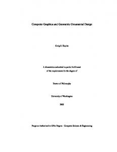
7.4. Example

p4

0

1

1

Let us have a look on an example with 5 points.

p5

-1

0

2

→ Bs = λs The solution of the minimization problem is given as the Eigenvector of B that corresponds to the smallest Eigenvalue. ( see [6] for details )

Point

x

y

z

p1

1

0

0

p2

1

1

0

p3

0

0

1

p4

0

1

1

p5

-1

0

1

The result of the least squares calculation results in

S = −0.301511e1 + 0.301511e2 − 0.301511e3 −0.603023e∞ + 0.603023e0 Another representation of this object is S = −0.5e1 + 0.5e2 − 0.5e3 − e∞ + e0

Figure 9: Fit of a plane.


9

Now, the result is

S = 0.57735 ∗ e1 + 0.57735 ∗ e3 + 0.57735 ∗ e∞ representing a plane. ( see figure 9 )

8. Visual development of algorithms We use the OpenSource CLUCalc software to calculate with Geometric Algebra and to visualize the results of these calculations. CLUCalc is freely available for download at [13]. With the help of the CLUCalc Software you are able to edit and run Scripts called CLUScripts. A screenshot of CLUCalc can be seen in figure 10. 9. Conclusion In this paper, we solved our application problems using Geometric Computing. Therefore we transferred our 3D problem with the help of geometric intuition into the 5D Conformal Geometric Algebra and got our results back into the real 3D world. Geometric Computing is applicable in many different engineering scenarios and provides a straightforward and intuitive problem solving approach. References Figure 10: Screenshot of the CLUCalc windows

[1]

Bayro-Corrochano E. and Zamora J., A language of lines planes and spheres for visually guided robot manipulation and grasping. CINVESTAV, Unidad Guadalajara, GEOVIS Lab., Mexico, IROS 2004, Sendai, Japan, Sept. 2004

[2]

Dorst L. , Mann S. and Bouma Tim , GABLE: A Matlab Tutorial for Geometric Algebra, available at http://carol.wins.uva.nl/ leo/GABLE/

[3]

Dorst L. , Mann S. , Geometric Algebra: A Computational Framework for Geometrical Applications, IEEE Computer Graphics May/June and July August 2002

[4]

Leo Dorst, Chris Doran, Joan Lasenby, editors. Applications of Geometric Algebra in Computer Science and Engineerring. Birkhaeuser, 2002

[5]

Daniel Fontijne and Leo Dorst, Modeling 3D Euclidean Geometry, IEEE Computer Graphics and Applications, March/April 2003

[6]

Golub G. H. , van Loan C. F. , Matrix Computations, The Johns Hopkins University Press, Baltimore and London, 1996

[7]

Hestenes D. 2001. Old Wine in New Bottles: A New Algebraic Framework for Computational Geometry, in Geometric Algebra with applications in science and engineering Editors Bayro-Corrochano E. and Sobczyk G. Birkhauser, Boston, 2001

[8]

Hildenbrand D., Fontijne D., Perwass Ch., Dorst L. , Geometric Algebra and its Application to Computer Graphics.

CLUCalc provides the following three windows • editor window • visualization window • output window The Inverse Kinematics algorithm, described in this paper, is implemented using CLUCalc. The corresponding CLUScripts ( InverseKinematics.clu is the main file ) can be downloaded from the homepage http://www.gris.informatik.tudarmstadt.de/~dhilden/

There is almost a one to one correspondence between formulae and codes. E. g. the computations of step 3 are easily done as follows S1 = p0 - 0.5*d2*d2*einf; S2 = p2 - 0.5*d3*d3*einf; Pp1 = S1^S2^PI1; // choose one of the two points p1 = DissectSecond(*Pp1);

For details regarding CLUScript please refer to the CLUCalc online help [13].

10

Dietmar Hildenbrand / Geometric Computing in Computer Graphics Tutorial notes of the EUROGRAPHICS conference 2004 in Grenoble.

[9]

D. Hildenbrand, E. Bayro-Corrochano and J. Zamora, Advanced geometric approach for graphics and visual guided robot object manipulation, proceedings of ICRA 2005 International Conference on Robotics and Automation in Barcelona

[10]

H. Li, D. Hestenes and A. Rockwood. Generalized homogeneous coordinates for computational geometry, in [15] pages 27-52

[11]

E.M.S. Hitzer. Euclidean Geometric Objects in the Clifford Geometric Algebra of Origin, 3-Space, Infinity Bulletin of the Belgian Mathematical Society - Simon Stevin (2004)

[12]

Naeve and Rockwood, Geometric Algebra Siggraph 2001 course # 53

[13]

Perwass C. , CLUCalc Homepage Library, download from http://www.CluCalc.info, Cognitive Systems Group, University Kiel, 2004

[14]

Christian Perwass and Dietmar Hildenbrand, Aspects of Geometric Algebra in Euclidean, Projective and Conformal Space, An Introductory Tutorial, September 2003, Download http://www.informatik.uni-kiel.de/reports/2003/2003_tr10.pdf http://www.dgm.informatik.tu-darmstadt.de/staff/dietmar/

[15]

Sommer G., editor. Geometric Computing with Clifford Algebra. Springer Verlag Heidelberg, 2001

[16]

Suter J. , Geometric Algebra Primer, available at http://www.jaapsuter.com