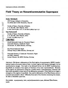
For an illustration see Fig. 1. g(x, t) x y w(x, y) f(g(x, t â D(x, y)/v)). Fig. 1. Diagram of a one dimen- sional neural field model. In this illustration the dendritic tree is.
Tutorial on neural field theory Stephen Coombes1 , Peter beim Graben2 , and Roland Potthast3 1 2 3
School of Mathematical Sciences, University of Nottingham, Nottingham, NG7 2RD, UK. Bernstein Center for Computational Neuroscience, 10115 Berlin, Germany. Department of Mathematics, University of Reading, RG6 6AX, UK.
Summary. The tools of dynamical systems theory are having an increasing impact on our understanding of patterns of neural activity. In this tutorial chapter we describe how to build tractable tissue level models that maintain a strong link with biophysical reality. These models typically take the form of nonlinear integro-differential equations. Their non-local nature has led to the development of a set of analytical and numerical tools for the study of spatiotemporal patterns, based around natural extensions of those used for local differential equation models. We present an overview of these techniques, covering Turing instability analysis, amplitude equations, and travelling waves. Finally we address inverse problems for neural fields to train synaptic weight kernels from prescribed field dynamics.
1 Background Ever since Hans Berger made the first recording of the human electroencephalogram (EEG) in 1924 [6] there has been a tremendous interest in understanding the physiological basis of brain rhythms. This has included the development of mathematical models of cortical tissue — which are often referred to as neural field models. One of the earliest of such models is due to Beurle [7] in the 1950s, who developed a continuum description of the proportion of active neurons in a randomly connected network. This was followed by work of Griffith [40, 41] in the 1960s, who also published two books that still make interesting reading for modern practitioners of mathematical neuroscience [42, 43]. However, it were Wilson and Cowan [90, 91] , Nunez [68] and Amari [3] in the 1970s who provided the formulations for neural field models that is in common use today. Usually, neural field models are conceived as neural mass models describing population activity at spatiotemporally coarse-grained scales [68, 91]. They can be classified as either activity-based [91] or voltage-based [3, 68] models (see [12, 64] for discussion). For their activity-based model Wilson and Cowan [90, 91] distinguished between excitatory and inhibitory sub-populations, as well as accounted for refractoriness. This seminal model can be written succinctly in terms of the pair of partial integro-differential equations: ∂E = −E + (1 − rE E)SE [wEE ⊗ E − wEI ⊗ I], ∂t ∂I = −I + (1 − rI I)SI [wIE ⊗ E − wII ⊗ I]. ∂t
(1)
2
Coombes, beim Graben & Potthast
Here E = E(r,t) is a temporal coarse-grained variable describing the proportion of excitatory cells firing per unit time at position r at the instant t. Similarly the variable I represents the activity of an inhibitory population of cells. The symbol ⊗ represents spatial convolution, the functions wab (r) describe the weight of all synapses to the ath population from cells of the bth population a distance |r| away, and ra is proportional to the refractory period of the ath population (in units of the population relaxation rate). The nonlinear function Sa describes the expected proportion of neurons in population a receiving at least threshold excitation per unit time, and is often taken to have a sigmoidal form. In many modern uses of the WilsonCowan equations the refractory terms are often dropped. For exponential or Gaussian choices of the connectivity function the Wilson-Cowan model is known to support a wide variety of solutions, including spatially and temporally periodic patterns (beyond a Turing instability), localised regions of activity (bumps and multi-bumps) and travelling waves (fronts, pulses, target waves and spirals), as reviewed in [17, 18, 29]. Further work on continuum models of neural activity was pursued by Nunez [68] and Amari [2, 3] under natural assumptions on the connectivity and firing rate function. Amari focused on local excitation and distal inhibition which is an effective model for a mixed population of interacting inhibitory and excitatory neurons with typical cortical connections (commonly referred to as Mexican hat connectivity), and formulated a single population (scalar) voltage-based model (without refractoriness) for activity u = u(r,t) of the form ∂u = −u + w ⊗ f (u), ∂t
(2)
for some sigmoidal firing rate function f and connectivity function w. For the case that f is a Heaviside step function he showed how exact results for localised states (bumps and travelling pulses) could be obtained. Since the original contributions of Wilson, Cowan, Nunez and Amari similar models have been used to investigate a variety of neural phenomena, including Electroencephalogram (EEG) and Magnetoencephalogram (MEG) rhythms [51, 52, 64, 67], geometric visual hallucinations [14, 30, 86], mechanisms for short term memory [62, 63], feature selectivity in the visual cortex [5], motion perception [36], binocular rivalry [54], and anaesthesia [65]. Neural field models have also found applications in autonomous robotic behaviour [27], embodied cognition [82], and dynamic causal modelling [25], as well as being studied from an inverse problems perspective [38, 75]. As well as an increase in the applications of models like (1) and (2) in neuroscience, there has been a push to develop a deeper mathematical understanding of their behaviour. This has led to results in one spatial dimension about the existence and uniqueness of bumps [58] and waves [31] with smooth sigmoidal firing rates, as well as some constructive arguments that generalise the original ideas of Amari for a certain class of smoothed Heaviside firing rate functions [21, 69]. Other mathematical work has focused on geometric singular perturbation analysis as well as numerical bifurcation techniques to analyse solutions in one spatial dimension [62, 72, 73]. More explicit progress has been possible for the case of Heaviside firing rate functions, especially as regards the stability of solutions using Evans functions [20]. The extension of results from one to two spatial dimensions has increased greatly in recent years [22, 34, 56, 60, 61, 70, 87]. This style of work has also been able to tackle physiological extensions of minimal neural field models to account for axonal delays [19, 48, 50, 68] (included in the original Wilson-Cowan model and then dropped for simplicity), dendritic processing [13], and synaptic depression [55]. In contrast to the analysis of spontaneously generated patterns of activity, relatively little work has been done on neural fields with forcing. The exceptions perhaps being the work in [35] (for localised drive) and global period forcing in [79]. However, much of the above work exploits idealisations of the
Tutorial on Neural Field Theory
3
original models (1) and (2), especially as regards heterogeneity and noise, to make mathematical progress. More recent work that tackles heterogeneity (primarily using simulations) can be found in [9], whilst perturbation theory and homogenisation techniques are developed in [11, 22, 81], and functional analytic results in [33]. The treatment of stochastic neural field models is a very new area, and we refer the reader to the recent review by Bressloff [12], which also covers methods from non-equilibrium statistical physics that attempt to move beyond the mean-field rate equations of the type exemplified by (1) and (2). However, it is fair to say that the majority of neural field models in use today can trace their roots back to the seminal work of Wilson and Cowan, Nunez and Amari. In this chapter we will develop the discussion of a particular neural field model that incorporates much of the spirit of (1) and (2), though with refinements that make a stronger connection to models of both synaptic and dendritic processing. We will then show how to analyse these models with techniques from dynamical systems before going on to discuss inverse problems in neural field theory.
1.1 Synaptic processing At a synapse, presynaptic firing results in the release of neurotransmitters that causes a change in the membrane conductance of the post-synaptic neuron. This post-synaptic current may be written Is = g(V −Vs ), (3) where V is the voltage of the post-synaptic membrane, Vs is its reversal potential and g is a conductance. This is proportional to the probability that a synaptic receptor channel is in an open conducting state. This probability depends on the presence and concentration of neurotransmitter released by the presynaptic neuron. The sign of Vs relative to the resting potential (assumed to be zero) determines whether the synapse is excitatory (Vs > 0) or inhibitory (Vs < 0). The effect of some synapses can be described with a function that fits the shape of the post-synaptic response due to the arrival of action potential at the pre-synaptic release site. A post-synaptic conductance change g(t) would then be given by g(t) = gη(t − T ),
t ≥ T,
(4)
where T is the arrival time of a pre-synaptic action potential and η(t) fits the shape of a realistic post-synaptic conductance. A common (normalised) choice for η(t) is a difference of exponentials: � � 1 −1 −αt 1 η(t) = − [e − e−βt ]H(t), (5) α β or the α-function :
η(t) = α 2 te−αt H(t),
(6)
where H is a Heaviside step function. The conductance change arising from a train of action potentials, with firing times Tm , is given by g(t) = g ∑ η(t − Tm ).
(7)
m
We note that both the forms for η(t) above can be written as the Green’s function of a linear differential operator, so that Qη = δ , where
4
Coombes, beim Graben & Potthast � �� � 1 d 1 d Q = 1+ 1+ , α dt β dt
(8)
for (5) and one simply sets β = α to obtain the response describing an α-function.
1.2 Dendritic processing Dendrites form the major components of neurons. They are complex branching structures that receive and process thousands of synaptic inputs from other neurons. It is well known that dendritic morphology plays an important role in the function of dendrites. A nerve fibre consists of a long thin, electrically conducting core surrounded by a thin membrane whose resistance to transmembrane current flow is much greater than that of either the internal core or the surrounding medium. Injected current can travel long distances along the dendritic core before a significant fraction leaks out across the highly resistive cell membrane. Conservation of electric current in an infinitesimal cylindrical element of nerve fibre yields a second-order linear partial differential equation (PDE) known as the cable equation. Let V (x,t) denote the membrane potential at position x along a uniform cable at time t measured relative to the resting potential of the membrane. Let τ be the cell membrane time constant, λ the space constant and r the membrane resistance, then the basic uniform (infinite) cable equation is τ
∂V (x,t) ∂ 2V (x,t) = −V (x,t) + λ 2 + rI(x,t), ∂t ∂ x2
x ∈ (−∞, ∞),
(9)
where we include the source term I(x,t) corresponding to external input injected into the cable. Diffusion along the dendritic tree generates an effective spatio-temporal distribution of delays as expressed by the associated Green’s function of the cable equation in terms of the diffusion constant D = λ 2 /τ. In response to a unit impulse at x0 at t = 0 and taking V (x, 0) = 0 the dendritic potential behaves as V (x,t) = G∞ (x − x0 ,t), where 2 1 G∞ (x,t) = √ e−t/τ e−x /(4Dt) H(t). 4πDt
(10)
The Green’s function G∞ (x,t) (derived in Appendix 1) determines the linear response to an instantaneous injection of unit current at a given point on the tree. Using the linearity of the cable equation one may write the general solution as Z t
V (x,t) = −∞
dt 0
Z ∞ −∞
dx0 G∞ (x − x0 ,t − t 0 )I(x0 ,t 0 ) +
Z ∞ −∞
dx0 G∞ (x − x0 ,t)V (x0 , 0).
(11)
Note that for notational simplicity we have absorbed a factor of r/τ within the definition of the source term I(x,t). For example, assuming the soma is at x = 0, V (x, 0) = 0 and the synaptic input is a train of spikes at x = x0 , I(x,t) = δ (x − x0 ) ∑m δ (t − Tm ) we have that V (0,t) = ∑ G∞ (x0 ,t − Tm ).
(12)
m
2 Tissue level firing rate models with axo-dendritic connections At heart modern biophysical theories assert that EEG signals from a single scalp electrode arise from the coordinated activity of ∼ 106 pyramidal cells in cortex [84]. These are arranged
Tutorial on Neural Field Theory
5
with their dendrites in parallel and perpendicular to the cortical surface. When synchronously activated by synapses at the proximal dendrites extracellular current flows (parallel to the dendrites), with a net membrane current at the synapse. For excitatory (inhibitory) synapses this creates a sink (source) with a negative (positive) extracellular potential. Because there is no accumulation of charge in the tissue the proximal synaptic current is compensated by other currents flowing in the medium causing a distributed source in the case of a sink and vice-versa for a synapse that acts as a source. Hence, at the population level the potential field generated by a synchronously activated population of cortical pyramidal cells behaves like that of a dipole layer. Although the important contribution that single dendritic trees make to generating extracellular electric field potentials has been realised for some time, and can be calculated using Maxwell’s equations [71], they are typically not accounted for in neural field models. The exception to this being the work of Bressloff, reviewed in [13]. In many neural population models it is assumed that the interactions are mediated by firing rates rather than action potentials (spikes) per se. To see how this might arise we rewrite (7) in the equivalent form Qg = g ∑ δ (t − Tm ). (13) m
If we perform a short-time average of (13) over some time-scale ∆ and assume that η is sufficiently slow so that hQgit is approximately constant, where hxit =
1 ∆
Z t
x(s)ds,
(14)
t−∆
then we have that Qg = f , where f is the instantaneous firing rate (number of spikes per time ∆ ). For a single neuron (real or synthetic) experiencing a constant drive it is natural to assume that this firing rate is a function of the drive alone. If for the moment we assume that a neuron spends most of its time close to rest such that Vs −V ≈ Vs , and absorb a factor Vs into g, then for synaptically interacting neurons this drive is directly proportional to the conductance state of the presynaptic neuron. Thus for a single population with self-feedback we are led naturally to equations like: Qg = w0 f (g), (15) for some strength of coupling w0 . A common choice for the population firing rate function is the sigmoid 1 f (g) = , (16) 1 + exp(−β (g − h)) which saturates to one for large g. This functional form, with threshold h and steepness parameter β , is approximately obtained for a unimodal distribution of firing thresholds among the population [90]. Note that the notion of a slow response would also be expected in a large globally coupled network which was firing asynchronously (so that mean field signals would be nearly constant). To obtain a tissue level model in one spatial dimension we simply consider g = g(x,t), with x ∈ R, and introduce a coupling function and integrate over the domain to obtain Z ∞
Qg =
w(x, y) f (g(y,t − D(x, y)/v))dy,
−∞
(17)
or equivalently Z t
g(x,t) = −∞
dsη(t − s)
Z ∞ −∞
w(x, y) f (g(y, s − D(x, y)/v))dy.
(18)
6
Coombes, beim Graben & Potthast
Here we have allowed for a communication delay, that arises because of the finite speed, v, of the action potential, where D(x, y) measures the length of the axonal fibre between points at x and y. The coupling function w(x, y) represents anatomical connectivity, and is often assumed to be homogeneous so that w(x, y) = w(|x − y|). It is also common to assume that D(x, y) = |x − y|. Following the original work of Bressloff (reviewed in [13]) we now develop the cable modelling approach of Rall [83] to describe a firing rate cortical tissue model with axodendritic patterns of synaptic connectivity. For simplicity we shall consider only an effective single population model in one (somatic) spatial dimension to include a further dimension representing position along a (semi-infinite) dendritic cable. The firing rate in the somatic (cell body) layer is taken to be a smooth function of the cable voltage at the soma, which is in turn determined by the spatio-temporal pattern of synaptic currents on the cable. For an illustration see Fig. 1.
f(g(x, t − D(x, y)/v))
g(x, t) x
y
w(x, y)
Fig. 1. Diagram of a one dimensional neural field model. In this illustration the dendritic tree is drawn with a branched structure. For the sake of simplicity the neural field model is only developed here for unbranched dendrites. However, this can be naturally generalised using the “sum-overtrips” approach of Abbott et al. for passive dendrites [1] and Coombes et al. [23] for resonant dendrites.
The voltage V (ξ , x,t) at position ξ ≥ 0 along a semi-infinite passive cable with somatic coordinate x ∈ R can then be written: V ∂ 2V ∂V = − + D 2 + I(ξ , x,t). ∂t τ ∂ξ
(19)
Here, I(ξ , x,t) is the synaptic input (and remember that we absorb within this a factor r/τ), and we shall drop shunting effects and take this to be directly proportional to a conductance change, which evolves according to the usual neural field prescription (cf equation (18)) as Z t
g(ξ , x,t) = −∞
dsη(t − s)
Z ∞ −∞
dyW (ξ , x, y) f (h(y, s − D(x, y)/v)).
(20)
The function W (ξ , x, y) describes the axo-dendritic connectivity pattern and the field h is taken as a measure of the drive at the soma. As a simple model of h we shall take it to be the somatic potential and write h(x,t) = V (0, x,t). For no flux boundary conditions ∂V (ξ , x,t)/∂ ξ |ξ =0 = 0, and assuming vanishing initial data, the solution to (19) at ξ = 0 becomes V (ξ = 0, x,t) = κ(G ⊗ g)(ξ = 0, x,t),
G = 2G∞
(21)
for some constant of proportionality κ > 0, where G∞ (x,t) is given by (10) and here the operator ⊗ denotes spatio-temporal convolution over the (ξ ,t) coordinates. Note that in
Tutorial on Neural Field Theory
7
obtaining (21) we have used the result that the Green’s function (between two points ξ and ξ 0 ) for the semi-infinite cable with no flux boundary conditions can be written as G∞ (ξ − ξ 0 ,t) + G∞ (ξ + ξ 0 ,t) [1, 88]. Further assuming that the axo-dendritic weights can be decomposed in the product form W (ξ , x, y) = P(ξ )w(|x − y|) then the equation for h takes the form Z t
h(x,t) = κ
−∞
dsF(t − s)
Z s −∞
ds0 η(s − s0 )
where
Z ∞ −∞
dyw(|x − y|) f (h(y, s0 − D(x, y)/v)),
(22)
Z ∞
F(t) =
dξ P(ξ )G(ξ ,t).
(23)
0
We regard equation (22) as a natural extension of the Amari model (2) to include synaptic and dendritic processing as well as axonal delays. Note that the Amari model is recovered from (22) in the limit v → ∞, η(t) = e−t H(t), and F(t) = δ (t)/κ.
2.1 Turing instability analysis To assess the pattern forming properties of the model given by (22) it is useful to perform a Turing instability analysis. This describes how a spatially homogeneous state can become unstable to spatially heterogeneous perturbations, resulting in the formation of periodic patterns. To illustrate the technique consider the one-dimensional model without dendrites or axonal delays, obtained in the limit v → ∞ and F(t) → δ (t): Z ∞
h(x,t) = κ
Z ∞
dsη(s) 0
−∞
dyw(|y|) f (h(x − y,t − s)).
(24)
One solution of the neural field equation is the spatially uniform resting state h(x,t) = h0 for all x,t, defined by Z ∞
h0 = κ f (h0 )
(25)
w(|y|)dy. −∞
Here we have used the fact that η is normalised, namely that 0∞ dsη(s) = 1. We linearise about this state by letting h(x,t) → h0 + h(x,t) so that f (h) → f (h0 ) + f 0 (h0 )u to obtain R
Z ∞
h(x,t) = κβ
Z ∞
dsη(s) 0
−∞
dyw(y)h(x − y,t − s),
β = f 0 (h0 ).
(26)
This has solutions of the form eλt eipx , with a dispersion curve: Z ∞
e (λ )w(p), b 1 = κβ η
b w(p) =
−∞
dyw(|y|)e−ipy ,
Z ∞
e (λ ) = η
dsη(s)e−λ s .
(27)
0
e as the Laplace transform of η. The b as the Fourier transform of w and η We recognise w uniform steady state is linearly stable if Reλ (p) < 0 for all p ∈ R, p 6= 0. For the choice e (λ ) = (1 + λ /α)−1 . In this case, since η(t) = αe−αt H(t) (so that Q = (1 + α −1 d/dt)) then η b w(x) = w(−x) then w(p) is a real even function of p and the stability condition is simply b w(p)
0 and this pattern grows with time. In fact there will typically exist a range of values of p ∈ (p1 , p2 ) for which λ (p) > 0, signalling a set of growing patterns. As the patterns grow, the linear approximation breaks down and nonlinear terms dominate the behaviour. The saturating property of f tends to create p patterns with finite amplitude, that scale as β − βc close to bifurcation and have wavelength 2π/pc . If pc = 0 then we would have a bulk instability resulting in the formation of another homogeneous state. ^
w(p) ^
Fig. 2. A plot of the Fourier transb form of the weight kernel w(p) illustrating how its shape (with a maximum away from the origin) can determine a Turing instability defined by the condition b c ) = 1. κβ w(p
1/ B > 1/Bc
increasing coupling ( )
wmax
1/
p
1/B < 1/Bc
p
1
2
pc
p
A common choice for w(x) is a Mexican hat function which represents short-range excitation and long-range inhibition. An example of such a function is a difference of two exponentials: h i w(x) = Λ e−γ1 |x| − Γ e−γ2 |x| , (29) with Γ < 1, γ1 > γ2 > 0 and Λ = +1. (The case Λ = −1, which represents short-range inhibition and long-range excitation will be considered below in the full model). The Fourier b transform w(p) is calculated as: " # γ1 γ2 b w(p) = 2Λ 2 −Γ 2 , (30) γ1 + p2 γ2 + p2 from which we may determine pc as p2c
=
p Γ γ2 /γ1 − γ22 p . 1 − Γ γ2 /γ1
γ12
(31)
Hence, pc 6= 0 when Γ > (γ2 /γ1 )3 . Note that for Λ = −1 then pc = 0 and a static Turing instability does not occur. For the full model (22) with D(x, y) = |x − y| the homogeneous steady state, h(x,t) = h0 for all x,t, satisfies Z Z ∞
h0 = κ f (h0 )
∞
F(s)ds −∞
0
dyw(|y|),
(32)
and the spectral equation takes the form Z ∞
e ), e (λ )F(λ b λ )η 1 = κβ w(p,
b λ) = w(p,
−∞
dyw(|y|)e−ipy e−λ |y|/v ,
β = f 0 (h0 ). (33)
Tutorial on Neural Field Theory
9
Compared to (27) it is now possible for complex solutions for λ to be supported – allowing for the possibility of dynamic (as opposed to static) Turing instabilities to occur. These occur when Im λ 6= 0 at the bifurcation point. b λ ) → w(p) b For example, in the limit v → ∞ then w(p, and for η(t) = αe−αt H(t) we have that e ). b F(λ 1 + λ /α = κβ w(p) (34) A necessary condition for a dynamic instability (Re λ = 0 and Im λ 6= 0) is that there exists a pair ω, p 6= 0 such that e b F(iω). 1 + iω/α = κβ w(p) (35) b Equating real and imaginary parts (and using the fact that w(p) ∈ R) gives us the pair of simultaneous equations b 1 = κβ w(p)C(ω),
b ω/α = κβ w(p)S(ω),
(36)
R∞
e e where C(ω) = Re F(iω) and S(ω) = Im F(iω). Note that C(ω) = 0 dsF(s) cos(ωs) ≤ |C(0)|. Hence (dividing the above equations) if there is a non-zero solution to ωc = H (ωc ), α
H (ωc ) ≡
S(ωc ) , C(ωc )
(37)
then the bifurcation condition, β = βd , for a dynamic instability is defined by b min ) = βd κ w(p
1 , C(ωc )
(38)
which should be contrasted with the bifurcation condition, β = βs , for a static instability, namely 1 b max ) = , (39) βs κ w(p C(0) where b min ) = min w(p), b b max ) = max w(p). b w(p w(p (40) p
p
b min ) < 0 < w(p b max ), a dynamic Turing instability will occur if β < βs and Assuming that w(p pmin 6= 0, whereas a static Turing instability will occur if βs < β and pmax 6= 0. For the Mexican hat function (29) with Λ = +1 (short-range excitation, long-range inhibition), a dynamic Turing instability is not possible since pmin = 0. However, it is possible for bulk oscillations to occur instead of static patterns when b c) < − w(p
C(ωc ) b |w(0)|, C(0)
(41)
with pc given by (31). On the other hand, when Λ = −1 (short-range inhibition, long-range excitation) a dynamic instability can occur since pmin = pc and pmax = 0, provided that b 0 from the soma). In this case F(t) = G(ξ0 ,t) with Laplace transform (calculated in Appendix 2): −γ(λ )ξ0 e )= e F(λ , Dγ(λ )
γ 2 (λ ) = (1/τ + λ )/D.
(43)
10
Coombes, beim Graben & Potthast
e In this case we may calculate the real and imaginary parts of F(iω) as 1
e−A+ (ω)ξ0 [A+ (ω) cos(A− (ω)ξ0 ) − A− (ω) sin(A− (ω)ξ0 )] 1/τ 2 + ω 2 1 S(ω) = − p e−A+ (ω)ξ0 [A+ (ω) sin(A− (ω)ξ0 ) + A+ (ω) cos(A− (ω)ξ0 )], 1/τ 2 + ω 2 p where (1/τ + iω)/D = A+ (ω) + iA− (ω) and rq C(ω) = p
A± (ω) =
[ 1/(τD)2 + ω 2 /D2 ± 1/(τD)]/2.
(44) (45)
(46)
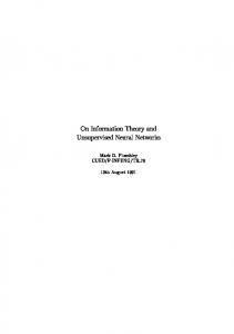
A plot of H(ω) is shown in Fig. 3, highlighting the possibility of a non-zero solution of (37) for a certain parameter set (and hence the possibility of a dynamic instability). Fig. 3. A plot of the function H(ω) for D = τ = 1 with ξ0 = 2, showing a non-zero solution of (37) for α = 1. This highlights the possibility of a dynamic Turing instability (ωc 6= 0) in a dendritic neural field model with shortrange inhibition and long-range excitation.
10 H(ω) 5 ωc 0 -5 -10 0
5
10
15
ω
20
For a discussion of dynamic Turing instabilities with finite v we refer the reader to [89]. For the treatment of more general forms of axo-dendritic connectivity (that do not assume a product form) we refer the reader to [10, 15]. The extension of the above argument to two dimensions shows that the linearised equations of motion have solutions of the form eλt eip·r , r, p ∈ R2 , with λ = λ (p), p = |p| as determined by (33) with Z
b λ) = w(p,
R2
drw(|r|)e−ip·r e−λ |r|/v .
(47)
Near bifurcation we expect spatially periodic solutions of the form exp i[p1 x + p2 y], p2c = p21 + p22 . For a given pc there are an infinite number of choices for p1 and p2 . It is therefore convenient to restrict attention to doubly periodic solutions that tessellate the plane. These can be expressed in terms of the basic symmetry groups of hexagon, square and rhombus. Solutions can then be constructed from combinations of the basic functions eipc R·r , for appropriate choices of the basis vectors R. If φ is the angle between two basis vectors R1 and R2 , we can distinguish three types of lattice according to the value of φ : square lattice (φ = π/2), rhombic lattice (0 < φ < π/2) and hexagonal (φ = π/3). Hence, all doubly periodic functions may be written as a linear combination of plane waves
Tutorial on Neural Field Theory h(r) = ∑ A j eipc R j ·r + cc,
|R j | = 1,
11 (48)
j
where√cc stands for complex-conjugate. For hexagonal lattices we use R1 = (1, 0), R2 = √ (−1, 3)/2, and R3 = (1, 3)/2. For square lattices we use R1 = (1, 0), R2 = (0, 1), while the rhombus tessellation uses R1 = (1, 0), R2 = (cos ζ , sin ζ ).
2.2 Weakly nonlinear analysis — amplitude equations A characteristic feature of the dynamics of systems beyond an instability is the slow growth of the dominant eigenmode, giving rise to the notion of a separation of scales. This observation is key in deriving the so-called amplitude equations. In this approach information about the short-term behaviour of the system is discarded in favour of a description on some appropriately identified slow time-scale. By Taylor-expansion ofpthe dispersion curve near its maximum one expects the scalings Re λ ∼ β − βc , p − pc ∼ β − βc , close to bifurcation, where β is the bifurcation parameter. Since the eigenvectors at the point of instability are of the type A1 ei(ωc t+pc x) + A2 ei(ωc t−pc x) + cc, for β > βc emergent patterns are described by an√infinite sum of unstable modes (in a continuous band) of the form eν0 (β −βc )t ei(ωc t+pc x) eip0 β −βc x . Let us denote β = βc + ε 2 δ where ε is arbitrary and δ is a measure of the distance from the bifurcation point. Then, for small ε we can separate the dynamics into fast eigen-oscillations 2 ei(ωc t+pc x) , and slow modulations of the form eν0 ε t eip0 εx . If we set as further independent variables τ = ε 2 t for the modulation time-scale and χ = εx for the long-wavelength spatial scale (at which the interactions between excited nearby modes become important) we may write the weakly nonlinear solution as A1 (χ, τ)ei(ωc t+pc x) + A2 (χ, τ)ei(ωc t−pc x) + cc. It is known from the standard theory [47] that weakly nonlinear solutions will exist in the form of either travelling waves (A1 = 0 or A2 = 0) or standing waves (A1 = A2 ). We are now in a position to derive the amplitude equations for patterns emerging beyond the point of an instability for a neural field model. These are also useful for determining the sub- or super-critical nature of the bifurcation. For clarity we shall first focus on the case of a static instability, and consider the example system given by (18) with η(t) = e−t H(t) and v → ∞, equivalent to the Amari model (2). In this case the model is conveniently written as an integro-differential equation: ∂g = −g + w ⊗ f (g), (49) ∂t where the symbol ⊗ denotes spatial convolution (assuming w(x, y) = w(|x − y|)). We first Taylor expand the nonlinear firing rate around the steady state g0 : f (g) = f (g0 ) + β1 (g − g0 ) + β2 (g − g0 )2 + β3 (g − g0 )3 + . . . ,
(50)
where β1 = f 0 (g0 ), β2 = f 00 (g0 )/2 and β3 = f 000 (g0 )/6. We also adopt the perturbation expansion g = g0 + εg1 + ε 2 g2 + ε 3 g3 + . . . . (51) After rescaling time according to τ = ε 2 t and setting β1 = βc + ε 2 δ , where βc is defined by b c ), we then substitute into (49). Equating powers of ε the bifurcation condition βc = 1/w(p leads to a hierarchy of equations:
12
Coombes, beim Graben & Potthast Z ∞
g0 = f (g0 )
(52)
w(|y|)dy, −∞
0 = L g1 ,
(53)
0 = L g2 + β2 w ⊗ g21 ,
(54)
dg1 = L g3 + δ w ⊗ g1 + 2β2 w ⊗ g1 g2 + β3 w ⊗ g31 , dτ
(55)
L g = −g + βc w ⊗ g.
(56)
where The first equation fixes the steady state g0 . The second equation is linear with solutions g1 = A(τ)eipc x + cc (where pc is the critical wavenumber at the static bifurcation). Hence the null space of L is spanned by e±ipc x . A dynamical equation for the complex amplitude A(τ) (and we do not treat here any slow spatial variation) can be obtained by deriving solvability conditions for the higher-order equations, a method known as the Fredholm alternative. These equations have the general form L gn = vn (g0 , g1 , . . . , gn−1 ) (with L g1 = 0). We define the inner product of two periodic functions (with periodicity 2π/pc ) as hU,V i =
pc 2π
Z 2π/pc
U ∗ (x)V (x)dx,
(57)
0
where ∗ denotes complex conjugation. It is simple to show that L is self-adjoint with respect to this inner product (see Appendix 3), so that hg1 , L gn i = hL g1 , gn i = 0.
(58)
Hence we obtain the set of solvability conditions he±ipc x , vn i = 0,
n ≥ 2.
(59)
b c )[A2 e2ipc x + The solvability condition with n = 2 is automatically satisfied, since w⊗g21 = w(2p b cc] + 2|A|2 w(0), and we make use of the result heimpc x , einpc x i = δm,n . For n = 3 the solvability condition (projecting onto e+ipc x ) is heipc x ,
dg1 − δ w ⊗ g1 i = β3 heipc x , w ⊗ g31 i + 2β2 heipc x , w ⊗ g1 g2 i. dτ
(60)
b c )[Aeipc x + cc], as The left-hand side is easily calculated, using w ⊗ g1 = w(p dA dA b c )A = − δ w(p − βc−1 δ A, dτ dτ
(61)
b c ). To evaluate the right-hand where we have made use of the bifurcation condition βc = 1/w(p b c )[A3 ei3pc x + cc] + 3|A|2 w(p b c )[Aeipc x + cc], to obtain side we use the result that w ⊗ g31 = w(p heipc x , w ⊗ g31 i = 3βc−1 A|A|2 . The next step is to determine g2 . From (54) we have that n o b c )[A2 e2ipc x + cc] + 2|A|2 w(0) b −g2 + βc w ⊗ g2 = −β2 w(2p .
(62)
(63)
We now set g2 = A+ e2ipc x + A− e−2ipc x + A0 + φ g1 .
(64)
Tutorial on Neural Field Theory
13
The constant φ remains undetermined at this order of perturbation but does not appear in the amplitude equation for A(τ). Substitution into (63) and equating powers of eipc x gives A0 =
b 2β2 |A|2 w(0) , b 1 − βc w(0)
A+ =
b c) β2 A2 w(2p , b c) 1 − βc w(2p
A− = A∗+ ,
(65)
b c )[A+ e2ipc x + A− e−2ipc x ] + w(0)A b where we have used the result that w ⊗ g2 = w(2p 0+ b c )eipc x + cc]. We then find that φ [Aw(p b c )[A+ A∗ + A0 A]. heipc x , w ⊗ g1 g2 i = w(p
(66)
Combining (61), (62) and (66) we obtain the Stuart-Landau equation βc
dA = A(δ − Φ|A|2 ), dτ
where Φ = −3β3 − 2β22
�
� b b c) 2w(0) w(2p + . b c ) 1 − βc w(0) b 1 − βc w(2p
(67)
(68)
Introducing A = Reiθ we may rewrite equation (67) as βc
dR = δ R − ΦR3 , dτ
dθ = 0. dτ
(69)
Hence, the phase of A is arbitrary (θ = const) and the amplitude has a pitchfork bifurcation which is super-critical for Φ > 0 and sub-critical for Φ < 0. Amplitude equations arising for systems with a dynamic instability are treated in [89]. The appropriate amplitude equations are found to be the coupled mean-field Ginzburg–Landau equations describing a Turing–Hopf bifurcation with modulation group velocity of O(1).
Amplitude equations for planar neural fields In two spatial dimensions the same ideas go across and can be used to determine the selection of patterns, say stripes vs. spots [28]. In the hierarchy of equations (52) to (55) the symbol ⊗ now represents a convolution in two spatial dimensions. The two dimensional Fourier transb takes the explicit form form w Z ∞
b 1 , p2 ) = w(p
Z ∞
−∞
dx
−∞
dyw(x, y)ei(p1 x+p2 y) ,
(70)
and the inner product for periodic scalar functions defined on the plane is taken as hU,V i =
1 |Ω |
Z
U ∗ (r)V (r)dr,
(71)
Ω
with Ω = (0, 2π/p �q c ) × (0, � 2π/pc ). We shall assume a radially symmetric kernel so that b (p1 , p2 ) = w b w p21 + p22 . One composite pattern that solves the linearised equations is g1 (x, y, τ) = A1 (τ)eipc x + A2 (τ)eipc y + cc.
(72)
For A1 = 0 and A2 6= 0 we have a stripe, while if both A1 and A2 are non-zero, and in particular b c ). The null space of equal, we have a spot. Here pc is defined by the condition βc = 1/w(p
14
Coombes, beim Graben & Potthast
L is spanned by {e±ipc x , e±ipc y }, and we may proceed as for the one dimensional case to generate a set of coupled equations for the amplitudes A1 and A2 . It is simple to show that heipc x , w ⊗ g31 i = 3βc−1 A1 (|A1 |2 + 2|A2 |2 ).
(73)
Assuming a representation for g2 as g2 = α0 + α1 e2ipc x + α2 e−2ipc x + α3 e2ipc y + α4 e−2ipc y + α5 eipc (x+y) + α6 e−ipc (x+y) + α7 eipc (x−y) + α8 e−ipc (x−y) + φ g1 ,
(74)
allows us to calculate heipc x , w ⊗ g1 g2 i = βc−1 [α0 A1 + α1 A∗1 + α5 A∗2 + α7 A2 ].
(75)
Balancing terms in (54) gives b c) β2 A21 w(2p , b c) 1 − βc w(2p √ b 2pc ) 2β2 A1 A∗2 w( √ α7 = . b 2pc ) 1 − βc w(
b 2β2 (|A1 |2 + |A2 |2 )w(0) , b 1 − βc w(0) √ b 2pc ) 2β2 A1 A2 w( √ , α5 = b 2pc ) 1 − βc w( α0 =
α1 =
(76) (77)
Combining the above yields the coupled amplitude equations: dA1 = A1 (δ − Φ|A1 |2 −Ψ |A2 |2 ), dτ dA2 βc = A2 (δ − Φ|A2 |2 −Ψ |A1 |2 ), dτ
βc
(78) (79)
where � b b c) 2w(0) w(2p + , b b c) 1 − βc w(0) 1 − βc w(2p # " √ b 2pc ) b 2w( w(0) 2 √ . Ψ = −6β3 − 4β2 + b 1 − βc w(0) b 2pc ) 1 − βc w( Φ = −3β3 − 2β22
�
(80) (81)
p The stripe solution A2 = 0 and |A1p | = δ /Φ (or vice versa) is stable if and only if Ψ > Φ > 0. The spot solution |A1 | = |A2 | = δ /(Φ +Ψ ) is stable if and only if Φ > Ψ > 0. Hence, stripes and spots are mutually exclusive as stable patterns. In the absence of quadratic terms in f , namely β2 = 0, then Ψ = −6β3 and Φ = −3β3 so that for an odd firing rate function like f (x) = tanh x ' x − x3 /3 then β3 < 0 and so Ψ > Φ and stripes are selected over spots. The key to the appearance of spots is non-zero quadratic terms, β2 6= 0, in the firing rate function; √ without these terms spots can never stably exist. For a Mexican hat connectivity b 2pc ) > w(2p b c ) and the quadratic term of Ψ is larger than that of Φ so that as |β2 | then w( increases then spots will arise instead of stripes. The technique above can also be used to determine amplitude equations for more general patterns of the form N
g1 (r, τ) =
∑ A j (τ)eip R ·r . c
j=1
For further discussion we refer the reader to [29, 86].
j
(82)
Tutorial on Neural Field Theory
15
2.3 Brain wave equations Given the relatively few analytical techniques for investigating neural field models one natural step is to make use of numerical simulations to explore system dynamics. For homogeneous models we may exploit the convolution structure of interactions to develop fast Fourier methods to achieve this. Indeed we may also exploit this structure further to obtain equivalent PDE models [61], and recover the Brain wave equation often used in EEG modelling [49, 68]. For example consider a one-dimensional neural field model with axonal delays: Z ∞
Qg = ψ,
ψ(x,t) =
−∞
dyw(|x − y|) f (g(y,t − |x − y|)/v).
(83)
The function ψ(x,t) may be expressed in the form Z ∞
ψ(x,t) =
−∞
Z ∞
ds
−∞
dyG(x − y,t − s)ρ(y, s),
(84)
where G(x,t) = δ (t − |x|/v)w(x),
(85)
can be interpreted as another type of Green’s function, and we use the notation ρ(x,t) = f (g(x,t)).
(86)
Introducing Fourier transforms of the following form ψ(x,t) =
1 (2π)2
Z ∞ Z ∞ −∞ −∞
ei(kx+ωt) ψ(k, ω)dkdω,
(87)
allows us to write ψ(k, ω) = G(k, ω)ρ(k, ω),
(88)
assuming the Fourier transform of f (u) exists. It is straightforward to show that the Fourier transform of (85) is G(k, ω) = ν(ω/v + k) + ν(ω/v − k), (89) where
Z ∞
ν(E) =
w(x)e−iEx dx.
(90)
0
We shall focus on a common form of (normalised) exponential synaptic footprint: w(x) =
1 exp(−|x|/σ ), 2σ
ν(E) =
1 1 , 2σ σ −1 + iE
σ > 0.
(91)
We now exploit the product structure of (88) and properties of (89) to re-formulate the original integral model in terms of a PDE. Using (89) and (91) we see that G(k, ω) =
A(ω) 1 , σ A(ω)2 + k2
A(ω) =
1 ω +i . σ v
(92)
We may now write (88) as (A(ω)2 + k2 )ψ(k, ω) = A(ω)ρ(k, ω)/σ , which upon inverse Fourier transforming gives the PDE: � � h i 1 1 1 A 2 − ∂xx ψ = A ρ, A = + ∂t . (93) σ σ v
16
Coombes, beim Graben & Potthast
This is a type of damped wave equation with an inhomogeneity dependent on (86). This equation has previously been derived by Jirsa and Haken [49] and studied intensively in respect to the brain-behaviour experiments of Kelso et al. [53]. For the numerical analysis of travelling wave solutions to (93) we refer the reader to [19]. The same approach can also be used in two spatial dimensions, and here G(k, ω) = G(k, ω) would be interpreted as the three dimensional integral transform: Z ∞
G(k, ω) =
−∞
Z
ds
R2
drG(r, s)e−i(k·r+ωs) .
(94)
For the choice w(r) = e−r/σ /(2π), we find that (see Appendix 4) G(k, ω) =
A(ω) (A2 (ω) + k2 )3/2
,
(95)
which, unlike in one spatial dimension, is not a ratio of polynomials in k and ω. The problem arises as of how to interpret [A 2 − ∇2 ]3/2 . In the long-wavelength approximation one merely expands G(k, ω) around k = 0 for small k, yielding a “nice” rational polynomial structure which is then manipulated as described above to give the PDE: � � 3 A 2 − ∇2 ψ = ρ. (96) 2 This model has been intensively studied by a number of authors in the context of EEG modelling, see for example [8, 78, 85]. For an alternative approximation to the long-wavelength one we refer the reader to [24].
3 Travelling waves and localised states As well as global periodic patterns neural field models are able to support localised solutions in the form of standing bumps and travelling pulses of activity. For clarity of exposition we shall focus on a one-dimensional neural field model with axonal delays: Z ∞
g(x,t) = −∞
Z ∞
dyw(y)
dsη(s) f ◦ g(x − y,t − s − |y|/v).
(97)
0
Following the standard approach for constructing travelling wave solutions to PDEs, such as reviewed by Sandstede [80], we introduce the coordinate ξ = x − ct and seek functions U(ξ ,t) = g(x − ct,t) that satisfy (97). In the (ξ ,t) coordinates, the integral equation (97) reads Z ∞ Z ∞ U(ξ ,t) = dyw(y) dsη(s) f ◦U(ξ − y + cs + c|y|/v,t − s − |y|/v). (98) −∞
0
The travelling wave is a stationary solution U(ξ ,t) = q(ξ ) (independent of t), that satisfies Z ∞
q(ξ ) =
Z ∞
η(s)ψ(ξ + cs)ds, 0
ψ(ξ ) =
−∞
w(y) f ◦ q(ξ − y + c|y|/v)dy.
(99)
To determine stability we linearise (98) about the steady state q(ξ ) by writing U(ξ ,t) = q(ξ ) + u(ξ ,t), and Taylor expand, to give Z ∞
u(ξ ,t) = −∞
Z ∞
dyw(y)
dsη(s) f 0 (q(ξ − y + cs + c|y|/v))u(ξ − y + cs + c|y|/v,t − s − |y|/v).
0
(100)
Tutorial on Neural Field Theory
17
Of particular importance are bounded smooth solutions defined on R, for each fixed t. Thus one looks for solutions of the form u(ξ ,t) = u(ξ )eλt . This leads to the eigenvalue equation u = L u: ds η(−ξ /c+y/c−|y|/v+s/c)e−λ (−ξ /c+y/c+s/c) f 0 (q(s))u(s). −∞ ξ −y+c|y|/v c (101) Let σ (L ) be the spectrum of L . We shall say that a travelling wave is linearly stable if Z ∞
u(ξ ) =
Z ∞
dyw(y)
max{Re(λ ) : λ ∈ σ (L ), λ 6= 0} ≤ −K,
(102)
for some K > 0, and λ = 0 is a simple eigenvalue of L . In general the normal spectrum of the operator obtained by linearising a system about its travelling wave solution may be associated with the zeros of a complex analytic function, the so-called Evans function. This was originally formulated by Evans [32] in the context of a stability theorem about excitable nerve axon equations of Hodgkin-Huxley type. Next we show how to calculate the properties of waves and bumps for the special case of a Heaviside firing rate function, f (g) = H(g − h), for some constant threshold h.
3.1 Travelling front As an example consider travelling front solutions such that q(ξ ) > h for ξ < 0 and q(ξ ) < h for ξ > 0. It is then a simple matter to show that (R ∞ w(y)dy ξ ≥ 0 . (103) ψ(ξ ) = Rξ∞/(1−c/v) ξ /(1+c/v) w(y)dy ξ < 0 The choice of origin, q(0) = h, gives an implicit equation for the speed of the wave as a function of system parameters. The construction of the Evans function begins with an evaluation of (101). Under the change of variables z = q(s) this equation may be written Z q(∞)
dz η(q−1 (z)/c − ξ /c + y/c − |y|/v) c −1 δ (z − h) × e−λ (q (z)/c−ξ /c+y/c) 0 −1 u(q−1 (z)). |q (q (z))| Z ∞
u(ξ ) =
−∞
dyw(y)
q(ξ −y+c|y|/v)
(104)
For the travelling front of choice we note that when z = h, q−1 (h) = 0 and (104) reduces to u(ξ ) =
u(0) c|q0 (0)|
Z ∞ −∞
dyw(y)η(−ξ /c + y/c − |y|/v)e−λ (y−ξ )/c .
(105)
From this equation we may generate a self-consistent equation for the value of the perturbation at ξ = 0, simply by setting ξ = 0 on the left hand side of (105). This self-consistent condition reads Z ∞ u(0) u(0) = dyw(y)η(y/c − |y|/v)e−λ y/c . (106) 0 c|q (0)| −∞ Importantly there are only nontrivial solutions if E (λ ) = 0, where E (λ ) = 1 −
1 c|q0 (0)|
Z ∞ −∞
dyw(y)η(y/c − |y|/v)e−λ y/c .
(107)
18
Coombes, beim Graben & Potthast
From causality η(t) = 0 for t ≤ 0 and physically c < v so E (λ ) = 1 −
1 c|q0 (0)|
Z ∞
dyw(y)η(y/c − y/v)e−λ y/c .
(108)
0
We identify (108) with the Evans function for the travelling front solution of (97). The Evans function is real-valued if λ is real. Furthermore, (i) the complex number λ is an eigenvalue of the operator L if and only if E (λ ) = 0, and (ii) the algebraic multiplicity of an eigenvalue is equal to the order of the zero of the Evans function. Consider the choice η(t) = e−t H(t) and w(x) = e−|x| /2. Assuming c > 0 the travelling front (99) is given in terms of (103) which takes the explicit form ( 1 m− ξ e ξ ≥0 v ψ(ξ ) = 2 1 m ξ , m± = . (109) c±v 1− 2e + ξ 0 showing that λ = 0 is a simple eigenvalue. Hence, the travelling wave front for this example is linearly stable. We refer the reader to [20] for further examples of wave calculations in other neural field models. R
3.2 Stationary bump Here we construct static (time-independent) patterns of the form g(x,t) = q(x) for all t. Using (97) gives Z ∞
w(x − y)H(q(y) − h)dy.
q(x) = −∞
(112)
We shall assume the synaptic kernel has a Mexican hat shape given by w(x) = (1 − |x|)e−|x| ,
(113)
and look for solutions of the form limx→±∞ q(x) = 0, with q(x) ≥ h for x1 < x < x2 (see inset of Fig. 4). In this case the exact solution is given simply by Z x2
q(x) =
w(x − y)dy.
(114)
x1
For the Mexican hat function (113), a simple calculation gives g(x − x1 ) − g(x − x2 ) x > x2 q(x) = g(x2 − x) + g(x − x1 ) x1 ≤ x ≤ x2 , g(x2 − x) − g(x1 − x) x < x1
(115)
Tutorial on Neural Field Theory
19
where g(x) = xe−x . The conditions q(x1 ) = h and q(x2 ) = h both lead to the equation ∆ e−∆ = h,
(116)
describing a family of solutions with ∆ = (x2 − x1 ). Hence, homoclinic bumps are only possible if h < 1/e. The full branch of solutions for ∆ = ∆ (h) is shown in Fig. 4. Here we see a branch of wide solutions (∆ > 1) and a branch of thinner solutions (∆ < 1) that connect in a saddle-node bifurcation at ∆ = 1. One of the translationally invariant solutions may be picked Fig. 4. Bump width as a function of h, as determined by equation (116) for a step function firing rate function and Mexican hat kernel (113). The inset shows the shape of a bump. A linear stability analysis shows that the upper branch of solutions is stable, and the lower branch unstable.
6 ∆ h
4
∆ 2
0 0
0.1
0.2
0.3
h
0.4
by imposing a phase condition q(0) = q0 , where q0 ≤ max q(x) = ∆ e−∆ /2 (which occurs at (x1 + x2 )/2 using (115)). To determine stability we use the result that q0 (x) = w(x − x1 ) − w(x − x2 ) so that the eigenvalue equation (101), with c = 0, reduces to u(x) =
e (λ ) η [w(x − x1 )u(x1 )e−λ |x−x1 |/v + w(x − x2 )u(x2 )e−λ |x−x2 |/v ], |w(0) − w(∆ )|
(117)
e (λ ) = 0∞ η(s)e−λ s ds. The equality in (117) implies that if u(x1,2 ) = 0 then u(x) = 0 where η for all x. We now examine the matrix equation obtained from (117) at the points x = x1,2 , R
� � � �� � e (λ ) η w(0) w(∆ )e−λ |∆ |/v u(x1 ) u(x1 ) = . u(x2 ) u(x2 ) |w(0) − w(∆ )| w(∆ )e−λ |∆ |/v w(0)
(118)
Non-trivial solutions are only possible if 1 w(0) ± w(∆ )e−λ |∆ |/v = . e |w(0) − w(∆ )| η (λ )
(119)
Solutions will be stable if Re(λ ) < 0. It is a simple matter to check that there is always e (λ ) = (1 + λ /α)−1 and we see that one solution with λ = 0. For an exponential synapse η as v → ∞ solutions are only stable if (w(0) + w(∆ ))/|w(0) − w(∆ )| < 1. This is true if w(∆ ) = exp(−∆ )(1 − ∆ ) < 0. Hence, of the two possible branches of ∆ = ∆ (h), it is the
20
Coombes, beim Graben & Potthast
one with largest ∆ that is stable. In the other extreme where v → 0 it is simple to show that real and positive values for λ can only occur when w(∆ ) > 0. Hence, as v is varied there are no new instabilities due to real eigenvalues passing through zero. However, for finite conduction velocities it is possible that solutions may destabilise via a Hopf bifurcation. By writing λ = iω the conditions for a Hopf bifurcation, where Re(λ ) = 0 and Im(λ ) 6= 0, are obtained from the simultaneous solution of 1=
w(0) + w(∆ ) cos(ω|∆ |/v) , |w(0) − w(∆ )|
ω w(∆ ) sin(ω|∆ |/v) =− . α |w(0) − w(∆ )|
(120)
Eliminating sin(ω|∆ |/v) between these two equations gives ω2 =
h i α2 2 2 w (∆ ) − {|w(0) − w(∆ )| − w(0)} . |w(0) − w(∆ )|2
(121)
The condition that ω 6= 0 requires the choice w(∆ ) > w(0), which does not hold for (113). Hence, the presence of axonal delays neither affects the existence or stability of bump solutions.
3.3 Interface dynamics For zero axonal delays (v → ∞) and η(t) = αe−αt H(t) the existence and stability of bumps may be investigated using the alternative techniques of Amari [3]. We use the threshold condition g(xi ,t) = h to define the locations x1,2 from which we obtain the equations of motion of the boundary as dxi gt = − . (122) dt gx x=xi (t)
It is then possible to calculate the rate of change of the interval ∆ (t) = x2 (t) − x1 (t) using 1 gt (x,t) = −g(x,t) + α
Z x2 (t)
w(x − y)dy.
(123)
� w(|y|)dy − h ,
(124)
x1 (t)
Then (for a single bump) d∆ =α dt
�
1 1 + c1 c2
� �Z
∆
0
where
∂ g(x1 ,t) ∂ g(x2 ,t) , −c2 = . (125) ∂x ∂x Hence, making the convenient assumption that ∂ g(xi ,t)/∂ x is roughly constant, the equilibR rium solution defined by 0∆ w(|y|)dy = h is stable if c1 =
d d∆
Z ∆
w(|y|)dy = w(∆ ) < 0.
(126)
0
We thus recover the result obtained with the Evans function method (widest bump is stable). It is also possible to recover results about travelling fronts in the interface framework (at least for v → ∞). In this case it is natural to define a pattern boundary as the interface between a high and low activity state. Let us assume that the front is such that g(x,t) > h for x < x0 (t) and g(x,t) ≤ h for x ≥ x0 (t) then (97), for the choice η(t) = e−t H(t), reduces to
Tutorial on Neural Field Theory gt (x,t) = −g(x,t) +
21
Z ∞
w(y)dy.
(127)
x−x0 (t)
Introducing z = ux and differentiating (127) with respect to x gives zt (x,t) = −z(x,t) − w(x − x0 (t)).
(128)
Integrating (128) from −∞ to t (and dropping transients) gives z(x,t) = −e−t
Z t −∞
es w(x − x0 (s))ds.
We may now use the interface dynamics, g(x0 (t),t), defined by: gt , x˙0 = − gx x=x0 (t)
(129)
(130)
to study the speed c > 0 of a front, defined by x˙0 = c. In this case x0 (t) = ct (where without loss of generality we set x0 (0) = 0) and from (127) and (128) we have that e gt |x=x0 (t) = −h + w(0), e )= where w(λ the equation
e gx |x=x0 (t) = −w(1/c)/c,
(131)
R ∞ −λ s w(s)ds. Hence from (130) the speed of the front is given implicitly by 0 e
e − w(1/c). e h = w(0)
(132)
To determine stability of the travelling wave we consider a perturbation of the interface and an associated perturbation of g. Introducing the notation b· to denote perturbed quantities to a first approximation we will set gbx |x=bx0 (t) = gx |x=ct , and write xb0 (t) = ct + δ x0 (t). The perturbation in g can be related to the perturbation in the interface by noting that the perturbed and unperturbed boundaries are defined by a level set condition so that g(x0 ,t) = h = gb(b x0 ,t). Introducing δ g(t) = g|x=ct − gb|x=bx0 (t) we thus have the condition that δ g(t) = 0 for all t. Integrating (127) (and dropping transients) gives g(x,t) = e−t
Z t −∞
dses
Z ∞
dyw(y),
(133)
x−x0 (s)
and gb is obtained from (133) by simply replacing x0 by xb0 . Using the above we find that δ u is given (to first order in δ x0 ) by δ g(t) =
1 c
Z ∞ 0
dse−s/c w(s)[δ x0 (t) − δ x0 (t − s/c)] = 0.
(134)
This has solutions of the form δ x0 (t) = eλt , where λ is defined by E (λ ) = 0, with E (λ ) = 1 −
e + λ )/c) w((1 . e w(1/c)
(135)
A front is stable if Reλ < 0. e ) = (λ + 1)−1 /2. In this As an example consider the choice w(x) = e−|x| /2, for which w(λ case the speed of the wave is given from (132) as c=
1 − 2h , 2h
(136)
22
Coombes, beim Graben & Potthast
and λ . (137) 1+c+λ Note that these results are recover equations (110) and (111) in the limit v → ∞, as expected. Hence, the travelling wave front for this example is neutrally stable. For a recent extension of the Amari interface dynamics to planar neural field models we refer the reader to [22]. E (λ ) =
4 Inverse Neural Modelling While neural modelling is concerned with the study of the dynamics which arise in the framework of neural activity on the basis of some given connectivity function w, inverse neural modelling studies the construction of such connectivity kernels w(x, y) given a prescribed dynamics of the activity fields u(x,t).
4.1 Inverse Problems Here, we focus on the investigation of a kernel construction for the Amari equation (2) with a homogeneous kernel function w or its inhomogeneous version τ
∂u (x,t) = −u(x,t) + ∂t
Z
w(x, y) f (u(y,t))dy, x ∈ D,t ≥ 0,
(138)
D
with some constant τ > 0, where D ⊂ Rm is some bounded domain in space dimension m ∈ N. Let us assume that on D the field u(x,t) is given for x ∈ D,t ∈ [0, T ) with some final time T > 0. This is usually called the full field inverse neural problem. The task is to find a kernel w(x, y) such that the equation (138) with kernel w and initial condition u(x, 0) has u(x,t) as its unique solution for all x ∈ D and t ∈ [0, T ). Since u(x,t) is given, we can define ψ(x,t) := τ
∂u (x,t) + u(x,t), x ∈ D,t ∈ [0, T ) ∂t
(139)
and ϕ(x,t) := f (u(x,t)), x ∈ D,t ∈ [0, T ).
(140)
With the functions (139) and (140) we transform the dynamics (138) into Z
w(x, y)ϕ(y,t)dy, x ∈ D,t ∈ [0, T ).
ψ(x,t) =
(141)
D
The equation (141) is an integral equation for the unkown connectivity function w. We first remark that since the integration in (141) is carried out with respect to the variable y, and since the kernel ϕ(y,t) of the integral operator Z
(Kg)(t) :=
ϕ(y,t)g(y)dy, t ∈ [0, T ),
(142)
D
is dependent on y and t only, the spatial coordinate x ∈ D can be considered as a parameter, i.e. the integral equation is indeed a family of integral equations Kwx = ψ(x, ·), x ∈ D,
(143)
Tutorial on Neural Field Theory
23
with different left-hand sides ψ(x, ·) for x ∈ D, where we use the notation wx := w(x, ·). We need to answer questions of uniqueness, existence and stability for the inverse neural task. It will turn out, that the inverse neural field problem shares basic features with many other inverse problems as described for example in [16, 26, 57, 74]. Most inverse problems are ill-posed in the sense of Hadamard [44]. A problem is called well-posed, if 1) for given input data it has at most one solution (uniqueness), 2) for any input data there exists a solution (existence), 3) the solution depends continuously on the input data (stability). A problem which is not well-posed, is called ill-posed. Clearly, ill-posedness depends on the spaces under consideration, an appropriate condition can make non-unique problems uniquely solvable, the choice of appropriate norms can make an instable problem stable. But often, the spaces are dependent on the particular applied setup, and it is not possible to control input functions for example in spaces which need to take care of an infinite number of derivatives. This means that ill-posedness naturally appears in many inverse problems and needs to be taken care of. This is true also for the inverse neural field problem above. It is well-known [59] that a compact operator K : X → Y from an infinite dimensional normed space X into an infinite dimensional normed space Y cannot have a bounded inverse, since otherwise the identity operator I = K −1 ◦ K would be compact, which cannot be the case. Integral operators with continuous or weakly-singular kernels on bounded sets are compact in the spaces of continuous or L2 -integrable functions, since we find a sequence of finitedimensional approximations to the kernels. As a consequence we obtain compactness of the operator K defined in (142) in the spaces BC(D) and L2 (D). Thus, the inverse neural field problem under consideration is ill-posed in the sense described by the conditions 1) – 3). The kernel w does not depend stably on the right-hand side ψ ∈ BC(D) or ψ ∈ L2 (D). We need to stabilize the solution to the inverse problem, which is usually carried out by some regularization method. We will introduce regularization further down. Here, we first show that the inverse neural field problem is neither uniquely solvable nor is it exactly solvable at all in the general case where a function u(x,t) is prescribed (c.f. [38]). To see its non-uniqueness we consider the case where u(x,t) = 0 for x ∈ M and t ∈ [0, T ) on some set M ⊂ D. Let w˜ 6= 0 be a kernel which is zero for x, y 6∈ M and arbitrary for x, y ∈ M. Then, for a solution w1 (x, y) of the inverse problem the kernel w2 := w1 + w˜ 6= w2 is another different solution, since it does not change the dynamical behaviour of u. Thus, the inverse problem is non-unique. In general, the non-uniqueness can be characterized as follows. We define V := span{ϕ(·,t) : t ∈ [0, T )}
(144)
as a subset of L2 (D). Then, Kg = 0 can be written as hv, gi = 0 forall v ∈ V ⇔ g ∈ V ⊥ .
(145)
Thus, the inverse neural field problem is unique in L2 (D) if and only if V = L2 (D), which is equivalent to V ⊥ = {0}. It means that the time dynamics of the field ϕ(·,t) = f (u(·,t)) covers all dimensions of the space L2 (D). Any element w˜ of V ⊥ can be added to a solution kernel w and will not change the dynamics of the neural field u. Existence of solutions in a space X with for example X = L2 (D) or X = BC(D) is equivalent to the condition ψ(x, ·) ∈ K(X) for all x ∈ D. (146)
24
Coombes, beim Graben & Potthast
Assume that u(x, ·) ∈ Cn ([0, T )), but u(x, ·) 6∈ Cn+1 ([0, T )) and let f be analytic. Then Kg ∈ Cn ([0, T )) for any g ∈ L2 (D), but ψ = τ∂ u/∂t + u ∈ Cn−1 ([0, T )), ψ 6∈ Cn ([0, T )). As a consequence there cannot be a solution to the inverse neural field equation in L2 (D) in this case. In general the inverse neural field problem does not have a solution. But we will be able to construct approximate solutions. To this end we need to introduce regularization techniques. Consider a compact linear operator K : X → Y from a Hilbert space X into a Hilbert space Y . We denote its adjoint by K ∗ . Then, we denote the nonnegative square roots µn of the eigenvalues of the self-adjoint compact operator K ∗ K as singular values of the operator K, see for example [59]. We assume that µn are ordered according to its size, such that µ1 ≥ µ2 ≥ . . .. The singular vector for µn is denoted by vn , n ∈ N. Then, the set of vectors gn :=
1 Kvn , n ∈ N, µn
(147)
is an orthonormal system in Y , such that we have ∞
∑ µn hv, vn ign
Kv =
(148)
n=1
for elements v ∈ X. The equation (148) is known as the spectral representation of K with respect to its singular system. We also note that Kvn = µn gn , K ∗ gn = µn vn
(149)
for all n ∈ N. If K is injective, then the inverse of the operator K is given by K −1 g =
∞
1 hg, gn ivn µ n=1 n
(150)
∑
for an element g ∈ Y . If the operator K is compact, then the singular values µn need to tend to zero for n → ∞. This also means that 1/µn tends to infinity. The spectral coefficients hg, gn i of the function g ∈ Y are multiplied by a large number 1/µn , which reflects the unboundedness of the operator K −1 . The image space of K in Y is given by the elements g ∈ Y for which we have ∞
1 hg, gn i2 < ∞. 2 µ n=1 n
(151)
∑
Picard’s theorem (c.f. [16]) states that Kv = g has a solution in X if and only if (151) is satisfied for g ∈ Y . The basic idea of regulariation is to replace the unbounded term 1/µn in (150) by a bounded term. The method is called spectral damping, since it damps the unbounded modes of K −1 g. A regularization operator Rα : Y → X is defined by ∞
Rα g :=
(α)
∑ qn
hg, gn ivn .
(152)
n=1
(α)
Here, α > 0 is denoted as regularization parameter and the damping factors qn bounded for n ∈ N. The choice � 1 , n ≤ 1/α (α) qn := µn 0, otherwise,
need to be
(153)
Tutorial on Neural Field Theory
25
is known as spectral cut-off. The damping (α)
qn
µn , n ∈ N, α + µn2
:=
(154)
is known as Tikhonov regularization. In operator terms, Tiknonov regularization can be written as Rα = (αI + K ∗ K)−1 K ∗ , α > 0. (155) Tikhonov regularization can be equivalently obtained by minimizing the Tikhonov functional µα (v) := kvk2 + kKv − gk2
(156)
over v ∈ X. The minimizer vα of (156) is calculated by vα = Rα g. The operator Rα is a bounded operator from Y to X. It converges pointwise to the inverse K −1 , i.e. we have Rα g → K −1 g, α → ∞
(157)
for each g ∈ K(X), see for example [59], where one can also find the norm estimate 1 kRα k ≤ √ , α > 0. 2 α
(158)
From (154) we also observe that kRα k → ∞ for α → 0. We can now apply regularization to the solution of the integral equation family (143). With Rα defined via (155) we calculate a regularized reconstruction kernel wα (x, y) on x, y ∈ D by wα (x, ·) := Rα ψ(x, ·), x ∈ D.
(159)
Numerically, the reconstruction can be carried out using a grid xk , k = 1, ..., ND in the domain D and some time discretization t j , j = 1, ..., NT . Then, K is approximated by a matrix K in RNT ×ND and ψ(x,t) by a matrix Ψ in RND ×NT , where each column corresponds to a time t j , j = 1, ..., NT . The kernel w is approximated by a matrix W in RND ×ND , with entries wk,` which reflect the connectivity from y` to xk for k, ` ∈ {1, ..., ND }. Now, the integral equation (143) corresponds to the matrix equation KWT = Ψ T . (160) The regularized solution of (160) is calculated by WTα = (αI + KT K)−1 KT Ψ T .
(161)
Further regularization methods such as a gradient scheme, also known as backpropagation algorithm for neural learning, can be found in [38]. We close this methodological part by looking into a slightly more general form than (143). The task is to construct an integral operator Z
(W g)(x) :=
w(x, y)g(y)dy, x ∈ D
(162)
D
which maps a given family v j ∈ L2 (D), j ∈ J, of functions with some index set J into its images g j ∈ L2 (D), j ∈ J, i.e. we search W such that W v j = g j , j ∈ J.
(163)
26
Coombes, beim Graben & Potthast
Now consider some orthonormal system (ϕn )n∈N . If W is an integral operator, we can develop its kernel w(x, ·) into its Fourier series with respect to (ϕn )n∈N , i.e. � ∞ �Z w(x, y) = ∑ w(x, y)ϕn (y)dy ϕn (y) D
n=1 ∞
=
∑ (W ϕn )(x)ϕn (y)
n=1 ∞
=
∑ ψn (x)ϕn (y)
x, y ∈ D
(164)
n=1
with ψn (x) := (W ϕn )(x). This means that for every orthonormal system (ϕn )n∈N the kernel w is given by the sum over the products of ϕn (y) with its image element ψn (x), x, y ∈ D. The sum (164) is known as Hebbian learning rule in the framework of neural networks. It has originally been suggested by Hebb [46] as a mechanism based on physiological arguments. Here, it is a consequence of the Fourier theorem. Equation (164) shows that the Hebbian learning rule is exact for learning the dynamics on orthonormal patterns. Of coure, in general training patterns are no longer orthonormal and then the Hebb rule inhibits strong errors due to cross-talk between the patterns under consideration. In this case, the above approach based on regularization is the correct modification and extension of this approach which yields better and stable results. One important restriction for the task (163) needs to be noted at this point. Clearly, we have transformed the inverse problem into a linear equation. Assume that we have a state v which is linearly dependent on the states v1 , ..., vN . Then, we are not completely free to choose the image of v, but it is determined by the images of v j , for j = 1, ..., N via the consistency condition A � N � N W v = W ∑ α j v j = ∑ α jW v j . (165) j=1
j=1
Only if the consistency condition is satisfied, we can expect to obtain solvability of equation (163). A second important consistency condition B is coming from the time-dynamical aspect of the inverse problem. Of course, to excite some pulse at time t ∈ [0, T ), we need other pulses to be active in a neighborhood of t. The activity needs to be large enough such that the threshold given by the function f is reached. Thus, in the form (138) we cannot expect to obtain a solvable inverse problem, if the consistency conditions of type A and B are violated. We also refer to [75] for an interpretation of the above approach in terms of bi-orthogonal basis functions, which are numerically realized by the Moore-Penrose pseudo inverse given by K † := (K T K)−1 K T and which is stabilized by Tikhonov regularization (155) when K is an ill-posed operator as for the inverse neural field problem.
4.2 Cognitive Modelling Finally, we apply the inverse methods and its theory to problems of dynamic cognitive modelling as suggested in [37, 38, 75]. The basic task here is to gain a better understanding of cognitive processes by mapping them into a dynamic field environment. The dynamical fields are then understood as neural activity patterns, which leads to the above inverse neural field or neural kernel construction problem. The first step of dynamic cognitive modelling is to formulate some cognitive process in an abstract environment. In the easiest possible case we can consider a sequence of mental
Tutorial on Neural Field Theory
27
representations s j , j = 1, 2, ..., N j . These states live in some space Z, the mental state space. We now construct a structure preserving mapping ρ : Z → X into the Hilbert space X = L2 (D) of functions on a domain D. Here, we obtain a discrete sequence of states v j , j = 1, ..., N j in X. A continuous time dynamics can then be obtained by regarding the states v j as saddle nodes that are connected along a stable heteroclinic sequence (SHS) [77], using Haken’s order parameter approach [45]. Here, we employ either compactly supported functions χ : R → R of class C2 with χ(0) = 1 and χ(s) = 0 for |s| ≥ ∆t or Gaussians 2
χ(s) = e−σ s , s ∈ R,
(166)
and define a temporal dynamics by Nj
u(x,t) :=
∑ v j (x)χ(t − t j ),
x ∈ D,t ∈ [0, T ),
(167)
j=1
where t j are the points in time where the states v j have maximal excitation. We then solve the inverse neural field problem (141) with (167) as input. The result is a neural kernel w which generates the dynamical representation of the above cognitive process in activation space. An application of this approach to syntactic language processing and its tentative relation to event-related brain potentials can be found in [39]. More complicated processes can be carried out in a similar way. For example, we can study elementary logical activity such as OR, AND or XOR. The logical representation consists of variables a1 and a2 as input variables and an output variable b, which takes states in {0, 1} depending on the particular logical gate which we consider. The logical tables constitute our abstract logical space Z. As second step we map this space into a dynamical environment and construct a time-continuous dynamics. This is carried out by identifying the variables with coefficients of particular states v1 , v2 and vout in X = L2 (D). The dynamics can now be constructed as in (167), i.e. we choose times t = 0 on which the variables a1 and a2 take their input states, i.e. they are either equal to 1 or equal to 0 for vξ , ξ = 1, 2. The output time is set to t = T . Consistency. We now have to decide whether a direct transition from states at t = 0 to t = T leads to a consistend inverse problem. For the AND and for the OR operator this is feasible, but XOR cannot be realized directly due to the inconsistence of the corresponding image vectors as described in (165). The XOR logic in its simplest form tries to map (0, 0) 7→ 0,
(1, 0) 7→ 1,
(0, 1) 7→ 1,
(1, 1) 7→ 0
But the coefficients of the state (1, 1) of v1 and v2 are the linear combination of (1, 0) and (0, 1), i.e. we cannot reach 0 as its image coefficient for vout when we map (1, 0) onto 1 and (0, 1) onto 1 as well. We cannot expect to model the nonlinear XOR dynamics based on a linear equation. This observation has played a large role historically, when Minsky and Papert investigated the capabilities of the perceptron [66]. As shown in [75] in a neural field environment the problem has a simple solution by extending the dynamics. In a discrete environment this would correspond to the introduction of multi-layer networks, as it has been carried out for neural networks. Here, we employ two further states v3 and v4 , such that v1 , ..., v4 , vout are linearly independent. Then, we choose t1 := T /2 and decompose the task into the OR map from v1 , v2 onto v3 at time t1 , the AND map from v1 , v2 onto v4 at time t1 , a plain transition from v3 to vout and an inhibition from v4 to vout . Our dynamics within a time interval T /2 based on five linearly independent states can be written as
28
Coombes, beim Graben & Potthast (1) (0, 0, 0, 0, 0) 7→ (0, 0, 0, 0, 0), (2) (1, 0, 0, 0, 0) 7→ (0, 0, 1, 0, 0), (3) (0, 1, 0, 0, 0) 7→ (0, 0, 1, 0, 0), (4) (1, 1, 0, 0, 0) 7→ (0, 0, 1, 1, 0),
(5) (0, 0, 1, 0, 0) 7→ (0, 0, 0, 0, 1), (6) (0, 0, 0, 1, 0) 7→ (0, 0, 0, 0, 0), (7) (0, 0, 1, 1, 0) 7→ (0, 0, 0, 0, 0),
The time dynamics is now realized by an application of the rules in the interval [0,t1 ) first and then again in the interval [t1 , T ) based on the order parameter approach (167). We obtain a set of consistend pairs of states and their neuro-dynamical images. The result is a set of four dynamical activation patterns or neural fields u1 (x,t), ..., u4 (x,t) representing XOR, which are consistent with a neuro dynamical environment. We solve the inverse problem (141) or (160), respectively, to construct a kernel w(x, y) which now realizes the neural dynamics on the given states v1 , ..., v4 and vout . We show one possible realization with states which are Gaussian functions on the domain D = [0, 10] × [−5, 5] (k) 2
vk (x) = e−τ|x−z
|
, for k = 1, 2, vout (x) = e−τ|x−z
(out) 2
|
,
(168)
for x ∈ D with points z(1) = (0.2, 3), z(2) = (0.2, −3) and z(out) = (9, 0) and τ = 2 as well as (3) 2
˜ 1 −z1 v3 (x) = 0.5 · (1 + sin(2x2 ) · sin(2x1 )) · e−τ|x
|
,
2 ˜ 1 −z(3) −τ|x 2 |
v4 (x) = 0.5 · (1 + cos(2x2 ) · cos(2x1 )) · e
,
(169)
(3) z1
for x ∈ D with τ˜ = 0.3 and = 5. The time interval has been selected as [0, T ] with T = 10 and a choice of the order parameter functions (166) with σ = 2. The states v1 , v2 and vout are localized states in neural space. The states v3 and v4 are distributed space over some region of the neural space, which we have kept separate from the support of v1 , v2 and vout here for better visibility. This demonstrates that we can solve the inverse neural field problem with macrostates which are distributed over a large region of our neural space. We are not bound to localized neural pulses, as it is often used for neural modelling. For the numerical tests we have chosen nt = 40 time steps for the training and a discretization of n1 × n2 = 55 × 56 points in our neural space. Then, the calculations can be carried out R in some seconds in MATLAB . We show three time slices of the both the training pulses as well as their reconstruction via the neural field equation (138) in Figure 5. The plots are taken at the times t = 6 · nTt = 1.53, t = 18 · nTt = 4.62 and t = 36 · nTt = 9.23. To avoid an inverse crime (c.f. [16]), i.e. the testing of an inversion method on the same grid which was used to generate the data, here we have chosen a finer time-grid with nt = 80 for the neural field equation for carrying out the simulation after construction of the kernel w. Acknowledgement. SC would like to thank Ruth Smith for a careful reading of the material in this chapter. PbG gratefully acknowledges support from a DFG Heisenberg fellowship (GR 3711/1-2). The authors also thank EPSRC and the Centre for Cognitive Neuroscience and Neurodynamics (CINN) of the University of Reading, UK, for supporting the discussion on this tutorial by funding the 2nd International Conference on Neural Field Theory in April 2012 in Reading.
Appendix 1 The Green’s function for the infinite cable equation satisfies the PDE
Tutorial on Neural Field Theory
29
Fig. 5. We show three time slices of two pulses which enter the activation space at time t = 0 at states v1 and v2 . They lead to the excitation of the states v3 and v4 and then vout is excited or inhibited. The images show the original pattern (left) and the pattern which is generated by the neural field equation (right), where we used a time discretization which was finer than the training pattern to avoid an inverse crime.
Gt = −
G + DGxx , τ
G(x, 0) = δ (x).
(170)
If we introduce the Fourier transform Z ∞
G(k,t) = −∞
e−ikx G(x,t)dx,
G(x,t) =
1 2π
Z ∞ −∞
eikx G(k,t)dk
(171)
1 + Dk2 , τ
(172)
then we may obtain the ordinary differential equation Gt (k,t) = −ε(k)G(k,t),
G(k, 0) = 1,
ε(k) =
with solution G(k,t) = G(k, 0) exp(−ε(k)t). Performing an inverse Fourier transform gives G(x,t) =
1 2π
Z ∞ −∞
dkeikx e−ε(k)t = e−t/τ e−x
2
/4Dt
1 2π
Z ∞ −∞
2
e−Dt[k+ix/2Dt] dk
2 1 =√ e−t/τ e−x /(4Dt) , 4πDt
where we complete the square in (173) and use the fact that
(173) (174)
R∞
−∞ exp(−x
2 )dx = √π.
30
Coombes, beim Graben & Potthast
Appendix 2 Introducing the Laplace transform of of G(x,t) as G(x, λ ), where Z ∞
G(x, λ ) =
dse−λ s G(x, s),
(175)
0
means that we may transform (85) to obtain h i γ 2 (λ ) − dxx G(x, λ ) = δ (x)/D,
γ 2 (λ ) = (1/τ + λ )/D.
(176)
This second order ordinary differential equation has the solution G(x, λ ) =
e−γ(λ )|x| . 2Dγ(λ )
(177)
Appendix 3 Introduce periodic functions U(x) and V (x) and write using Fourier series as 2πinx/Λ and V (x) = ∞ U(x) = ∑∞ ∑n=−∞ Vn e2πinx/Λ , where Λ = 2π/pc . In this case, n=−∞ Un e [w ⊗V ](x) =
Z ∞ −∞
dyw(|y|)V (x − y)
Z ∞
=∑ n
−∞
dyw(|y|)Vn e2πin(x−y)/Λ
= ∑ Vn e2πinx/Λ wn , n
Z ∞
wn =
−∞
dyw(|y|)e−2πiny/Λ .
(178)
Hence, we may now calculate hU, w ⊗V i =
1 Λ
Z Λ 0
∑ Un∗ e−2πinx/Λ ∑ Vm wm e2πimx/Λ n
m
= ∑ Um∗ Vm wm ,
(179)
m
where we make use of the result that
R Λ 2πix(m−n)/Λ /Λ = δn,m . Similarly we find 0 e
hw ⊗U,V i = ∑ Um∗ Vm w∗m = hU, w ⊗V i,
(180)
m
where we make use of the fact that wm = w∗m . From (56) we have that hU, L V i = −hU,V i + βc hU, w ⊗V i = −hU,V i + βc hw ⊗U,V i = hL U,V i. Hence L is self-adjoint.
(181)
Tutorial on Neural Field Theory
31
Appendix 4 For w(r) = exp(−r/σ )/(2π) we may calculate equation (94) as G(k, ω) = (2π)−1
Z ∞
Z
dre−|r|/σ δ (s − |r|/v)e−i(k·r+ωs) ,
ds
−∞ R2 Z 2π Z ∞ −1 −ikr cos θ −Ar
= (2π)
e
0
0
e
rdrdθ = −(2π)−1
∂ ∂A
Z 2π 0
1 dθ , (182) A + ik cos θ
where A(ω) = 1/σ + iω/v. This may be evaluated using a (circular) contour integral in the complex plane to give A(ω) G(k, ω) = . (183) (A(ω)2 + k2 )3/2
References 1. Abbott, L.F., Fahri, E., Gutmann, S.: The path integral for dendritic trees. Biological Cybernetics 66, 49–60 (1991) 2. Amari, S.: Homogeneous nets of neuron-like elements. Biological Cybernetics 17, 211– 220 (1975) 3. Amari, S.: Dynamics of pattern formation in lateral-inhibition type neural fields. Biological Cybernetics 27, 77–87 (1977) 4. Anderson, J.A., Rosenfeld, E. (eds.): Neurocomputing. Foundations of Research, vol. 1. MIT Press, Cambridge (MA) (1988) 5. Ben-Yishai, R., Bar-Or, L., Sompolinsky, H.: Theory of orientation tuning in visual cortex. Proceedings of the National Academy of Sciences USA 92, 3844–3848 (1995) ¨ 6. Berger, H.: Uber das Elektroenkephalogramm des Menschen. Archiv f¨ur Psychiatrie 87, 527 – 570 (1929) 7. Beurle, R.L.: Properties of a mass of cells capable of regenerating pulses. Philosophical Transactions of the Royal Society London B 240, 55–94 (1956) 8. Bojak, I., Liley, D.T.J.: Modeling the effects of anesthesia on the electroencephalogram. Physical Review E 71, 041,902 (2005) 9. Brackley, C.A., Turner, M.S.: Random fluctuations of the firing rate function in a continuum neural field model. Physical Review E 75, 041,913 (2007) 10. Bressloff, P.C.: New mechanism for neural pattern formation. Physical Review Letters 76, 4644–4647 (1996) 11. Bressloff, P.C.: Traveling fronts and wave propagation failure in an inhomogeneous neural network. Physica D 155, 83–100 (2001) 12. Bressloff, P.C.: Spatiotemporal dynamics of continuum neural fields. Journal of Physics A 45, 033,001 (2012) 13. Bressloff, P.C., Coombes, S.: Physics of the extended neuron. International Journal of Modern Physics B 11, 2343–2392 (1997) 14. Bressloff, P.C., Cowan, J.D., Golubitsky, M., Thomas, P.J., Wiener, M.: Geometric visual hallucinations, Euclidean symmetry and the functional architecture of striate cortex. Philosophical Transactions of the Royal Society London B 40, 299–330 (2001) 15. Bressloff, P.C., Souza, B.D.: Neural pattern formation in networks with dendritic structure. Physica D 115, 124–144 (1998) 16. Colton, D., Kress, R.: Inverse acoustic and electromagnetic scattering theory, Applied Mathematical Sciences, vol. 93 Springer-Verlag, Berlin (1998)
32
Coombes, beim Graben & Potthast
17. Coombes, S.: Waves, bumps, and patterns in neural field theories. Biological Cybernetics 93, 91–108 (2005) 18. Coombes, S.: Large-scale neural dynamics: Simple and complex. NeuroImage 52, 731– 739 (2010) 19. Coombes, S., Lord, G.J., Owen, M.R.: Waves and bumps in neuronal networks with axodendritic synaptic interactions. Physica D 178, 219–241 (2003) 20. Coombes, S., Owen, M.R.: Evans functions for integral neural field equations with Heaviside firing rate function. SIAM Journal on Applied Dynamical Systems 34, 574–600 (2004) 21. Coombes, S., Schmidt, H.: Neural fields with sigmoidal firing rates: approximate solutions. Discrete and Continuous Dynamical Systems Series A 28, 1369–1379 (2010) 22. Coombes, S., Schmidt, H., Bojak, I.: Interface dynamics in planar neural field models. Journal of Mathematical Neuroscience 2(9) (2012) 23. Coombes, S., Timofeeva, Y., Svensson, C.M., Lord, G.J., Josic, K., Cox, S.J., Colbert, C.M.: Branching dendrites with resonant membrane: A “sum-over-trips” approach. Biological Cybernetics 97, 137–149 (2007) 24. Coombes, S., Venkov, N.A., Shiau, L., Bojak, I., Liley, D.T.J., Laing, C.R.: Modeling electrocortical activity through improved local approximations of integral neural field equations. Physical Review E 76, 051901 (2007). DOI 10.1103/PhysRevE.76.051901 25. Daunizeau, J., Kiebel, S.J., Friston, K.J.: Dynamic causal modelling of distributed electromagnetic responses. NeuroImage 47, 590–601 (2009) 26. Engl, H.W., Hanke, M., Neubauer, A.: Regularization of inverse problems, Mathematics and its Applications, vol. 375. Kluwer Academic Publishers Group, Dordrecht (1996) 27. Erlhagen, W., Bicho, E.: The dynamic neural field approach to cognitive robotics. Journal of Neural Engineering 3, R36–R54 (2006) 28. Ermentrout, B.: Stripes or spots? Nonlinear effects in bifurcation of reaction-diffusion equations on the square. Proceedings of the Royal Society of London. Series A 434, 413–417 (1991) 29. Ermentrout, G.B.: Neural nets as spatio-temporal pattern forming systems. Reports on Progress in Physics 61, 353–430 (1998) 30. Ermentrout, G.B., Cowan, J.D.: A mathematical theory of visual hallucination patterns. Biological Cybernetics 34, 137–150 (1979) 31. Ermentrout, G.B., McLeod, J.B.: Existence and uniqueness of travelling waves for a neural network. Proceedings of the Royal Society of Edinburgh 123A, 461–478 (1993) 32. Evans, J.: Nerve axon equations: IV The stable and unstable impulse. Indiana University Mathematics Journal 24, 1169–1190 (1975) 33. Faugeras, O., Grimbert, F., Slotine, J.J.: Absolute stability and complete synchronization in a class of neural fields models. SIAM Journal on Applied Mathematics 69, 205–250 (2008) 34. Folias, S.E., Bressloff, P.C.: Breathing pulses in an excitatory neural network. SIAM Journal on Applied Dynamical Systems 3, 378–407 (2004) 35. Folias, S.E., Bressloff, P.C.: Breathers in two-dimensional neural media. Physical Review Letters 95, 208,107(1–4) (2005) 36. Geise, M.A.: Neural Field Theory for Motion Perception. Kluwer Academic Publishers (1999) 37. beim Graben, P., Pinotsis, D., Saddy, D., Potthast, R.: Language processing with dynamic fields. Cognitive Neurodynamics 2(2), 79 – 88 (2008). 38. beim Graben, P., Potthast, R.: Inverse problems in dynamic cognitive modeling. Chaos 19(1), 015103 (2009).
Tutorial on Neural Field Theory
33
39. beim Graben, P., Potthast, R.: A dynamic field account to language-related brain potentials. In: Rabinovich et al. [76] 40. Griffith, J.S.: A field theory of neural nets: I: Derivation of field equations. Bulletin of Mathematical Biophysics 25, 111–120 (1963) 41. Griffith, J.S.: A field theory of neural nets: II: Properties of field equations. Bulletin of Mathematical Biophysics 27, 187–195 (1965) 42. Griffith, J.S.: A view of the brain. Oxford University Press (1967) 43. Griffith, J.S.: Mathematical Neurobiology. Academic Press (1971) 44. Hadamard, J.: Lectures on Cauchy’s problem in linear partial differential equations. Yale University Press, New Haven (1923) 45. Haken, H.: Principles of Brain Functioning, Springer Series in Synergetics, vol. 67. Springer, Berlin (1996) 46. Hebb, D.O.: The Organization of Behavior. Wiley, New York (NY) (1949). Partly reprinted in J. A. Anderson and E. Rosenfeld (1988), pp. 45ff. 47. Hoyle, R.: Pattern formation: An introduction to methods. Cambridge University Press (2006) 48. Hutt, A.: Effects of nonlocal feedback on traveling fronts in neural fields subject to transmission delay. Physical Review E 60, 052,902(1–4) (2004) 49. Jirsa, V.K., Haken, H.: Field theory of electromagnetic brain activity. Physical Review Letters 77, 960–963 (1996) 50. Jirsa, V.K., Haken, H.: A derivation of a macroscopic field theory of the brain from the quasi-microscopic neural dynamics. Physica D 99, 503 – 526 (1997) 51. Jirsa, V.K., Jantzen, K.J., Fuchs, A., Kelso, J.A.S.: Spatiotemporal forward solution of the EEG and MEG using network modeling. IEEE Transactions on Medical Imaging 21(5), 493 – 504 (2002). 52. Jirsa, V.K.V., Jantzen, K.J., Fuchs, A., Kelso, J.A.S.: Information Processing in Medical Imaging, chap. Neural Field Dynamics on the Folded Three-Dimensional Cortical Sheet and Its Forward EEG and MEG, pp. 286–299. Springer Berlin (2001) 53. Kelso, J.A.S., Bressler, S.L., Buchanan, S., Deguzman, G.C., Ding, M., Fuchs, A., Holroyd, T.: A phase-transition in human brain and behaviour. Physics Letters A 169, 134– 144 (1992) 54. Kilpatrick, Z.P., Bressloff, P.C.: Binocular rivalry in a competitive neural network with synaptic depression. SIAM Journal on Applied Dynamical Systems 9, 1303–1347 (2010) 55. Kilpatrick, Z.P., Bressloff, P.C.: Effects of synaptic depression and adaptation on spatiotemporal dynamics of an excitatory neuronal network. Physica D 239, 547–560 (2010) 56. Kilpatrick, Z.P., Bressloff, P.C.: Spatially structured oscillations in a two-dimensional excitatory neuronal network with synaptic depression. Journal of Computational Neuroscience 28, 193–209 (2010) 57. Kirsch, A.: An introduction to the mathematical theory of inverse problems, Applied Mathematical Sciences, vol. 120. Springer-Verlag, New York (1996) 58. Kishimoto, K., Amari, S.: Existence and stability of local excitations in homogeneous neural fields. Journal of Mathematical Biology 7, 303–318 (1979) 59. Kress, R.: Linear Integral Equations. Springer, Berlin (1989) 60. Laing, C.R.: Spiral waves in nonlocal equations. SIAM Journal on Applied Dynamical Systems 4, 588–606 (2005) 61. Laing, C.R., Troy, W.C.: PDE methods for nonlocal models. SIAM Journal on Applied Dynamical Systems 2, 487–516 (2003) 62. Laing, C.R., Troy, W.C.: Two bump solutions of Amari-type models of working memory. Physica D 178, 190–218 (2003)
34
Coombes, beim Graben & Potthast
63. Laing, C.R., Troy, W.C., Gutkin, B., Ermentrout, G.B.: Multiple bumps in a neuronal model of working memory. SIAM Journal on Applied Mathematics 63, 62–97 (2002) 64. Liley, D.T.J., Cadusch, P.J., Dafilis, M.P.: A spatially continuous mean field theory of electrocortical activity. Network: Computation in Neural Systems 13, 67 – 113 (2002) 65. Liley, D.T.J., Foster, B.L., Bojak, I.: Sleep and Anesthesia, chap. A Mesoscopic Modelling Approach to Anaesthetic Action on Brain Electrical Activity, pp. 139–166. Springer (2011) 66. Minsky, M., Papert, S.: Perceptrons. MIT Press, Cambridge (MA) (1969). Partly reprinted in J. A. Anderson and E. Rosenfeld (1988), pp. 161ff. 67. l Nunez, P.: Neocortical Dynamics and Human EEG Rhythms. Oxford University Press (1995) 68. Nunez, P.L.: The brain wave equation: a model for the EEG. Mathematical Biosciences 21, 279–297 (1974) 69. Oleynik, A., Posnov, A., Wyller, J.: Iterative schemes for bump solutions in a neural field model. submitted (2012) 70. Owen, M.R., Laing, C.R., Coombes, S.: Bumps and rings in a two-dimensional neural field: splitting and rotational instabilities. New Journal of Physics 9, 378 (2007) 71. Pettersen, K.H., Einevoll, G.T.: Amplitude variability and extracellular low-pass filtering of neuronal spikes. Biophysical Journal 94, 784–802 (2008) 72. Pinto, D.J., Ermentrout, G.B.: Spatially structured activity in synaptically coupled neuronal networks: I. Travelling fronts and pulses. SIAM Journal on Applied Mathematics 62, 206–225 (2001) 73. Pinto, D.J., Ermentrout, G.B.: Spatially structured activity in synaptically coupled neuronal networks: II. lateral inhibition and standing pulses. SIAM Journal on Applied Mathematics 62, 226–243 (2001) 74. Potthast, R.: Point sources and multipoles in inverse scattering theory, Chapman & Hall/CRC Research Notes in Mathematics, vol. 427. Chapman & Hall/CRC, Boca Raton, FL (2001) 75. Potthast, R., beim Graben, P.: Inverse problems in neural field theory. SIAM Jounal on Applied Dynamical Systems 8(4), 1405 – 1433 (2009). 76. Rabinovich, M., Friston, K., Varona, P. (eds.): Principles of Brain Dynamics: Global State Interactions. MIT Press, Cambridge (MA) (2012) 77. Rabinovich, M.I., Huerta, R., Varona, P., Afraimovich, V.S.: Transient cognitive dynamics, metastability, and decision making. PLoS Computational Biology 4(5), e1000,072 (2008). 78. Robinson, P.A., Rennie, C.J., Wright, J.J., Bahramali, H., Gordon, E., l Rowe, D.: Prediction of electroencephalographic spectra from neurophysiology. Physical Review E 63, 021,903 (2001) 79. Rule, M., Stoffregen, M., Ermentrout, B.: A model for the origin and properties of flickerinduced geometric phosphenes. PLoS Computational Biology 7(9), e1002,158 (2011) 80. Sandstede, B.: Handbook of Dynamical Systems II, chap. Stability of travelling waves, pp. 983–1055. Elsevier (2002) 81. Schmidt, H., Hutt, A., Schimansky-Geier, L.: Wave fronts in inhomogeneous neural field models. Physica D 238, 1101–1112 (2009) 82. Sch¨oner, G., Dineva, E.: Dynamic instabilities as mechanisms for emergence. Developmental Science 10, 69–74 (2007) 83. Segev, I., Rinzel, J., Shepherd, G.M. (eds.): The theoretical foundations of dendritic function: selected papers of Wilfrid Rall with commentaries. MIT Press (1995)
Tutorial on Neural Field Theory
35
84. da Silva, F.L., Rotterdam, A.V.: Electroencephalography: Basic principles, clinical applications and related fields, chap. Biophysical aspects of EEG and Magnetoencephalogram generation, pp. 107–126. Lippincott Williams & Wilkins (2005) 85. Steyn-Ross, M.L., Steyn-Ross, D.A., Sleigh, J.W., Liley, D.T.J.: Theoretical electroencephalogram stationary spectrum for a white-noise-driven cortex: Evidence for a general anesthetic-induced phase transition. Physical Review E 60, 7299–7311 (1999) 86. Tass, P.: Cortical pattern formation during visual hallucinations. Journal of Biological Physics 21, 177–210 (1995) 87. Taylor, J.G.: Neural ‘bubble’ dynamics in two dimensions: Foundations. Biological Cybernetics 80, 393–409 (1999) 88. Tuckwell, H.C.: Introduction to Theoretical Neurobiology Vol 1: Linear Cable Theory and Dendritic Structure. Cambridge University Press (1988) 89. Venkov, N.A., Coombes, S., Matthews, P.C.: Dynamic instabilities in scalar neural field equations with space-dependent delays. Physica D 232, 1–15 (2007) 90. Wilson, H.R., Cowan, J.D.: Excitatory and inhibitory interactions in localized populations of model neurons. Biophysical Journal 12, 1–24 (1972) 91. Wilson, H.R., Cowan, J.D.: A mathematical theory of the functional dynamics of cortical and thalamic nervous tissue. Kybernetik 13, 55–80 (1973)