2190
KSME International Journal, VoL 18, No. 12, pp. 2190--2203, 2004
Two-Dimensional Adaptive Mesh Generation Algorithm and its Application with Higher-Order Compressible Flow Solver Sutthisak Phongthanapanich, Pramote Dechaumphai* Mechanical Engineering Department, Chulalongkorn University, Bangkok 10330, Thailand
A combined procedure for two-dimensional Delaunay mesh generation algorithm and an adaptive remeshing technique with higher-order compressible flow solver is presented. A pseudo-code procedure is described for the adaptive remeshing technique. The flux-difference splitting scheme with a modified multidimensional dissipation for high-speed compressible flow analysis on unstructured meshes is proposed. The scheme eliminates nonphysical flow solutions such as the spurious bump of the carbuncle phenomenon observed from the bow shock of the flow over a blunt body and the oscillation in the odd-even grid perturbation in a straight duct for the Quirk's odd-even decoupling test. The proposed scheme is further extended to achieve higher-order spatial and temporal solution accuracy. The performance of the combined procedure is evaluated on unstructured triangular meshes by solving several steady-state and transient high-speed compressible flow problems. Key Words : Adaptive Mesh, Delaunay Triangulation, Carbuncle Phenomenon, H-correction Entropy Fix
1. Introduction Spatial discretization of a given domain is a prerequisite for solutions with finite-element or finite-volume method of a partial differential equations system that represents the physical model of the problem. Generally, triangulation process starts from the generation of the point list; the points are subsequently connected into triangular elements. The points connection step is often performed by constructing the Delaunay triangulation (Bowyer, 1981; Watson, 1981) of the point set to guarantee triangles which are as well-shaped as possible for the given points. Since the Delaunay triangulation in itself does not include procedures for creating points in-
* Corresponding Author, E-mail :
[email protected] Mechanical Engineering Department, Chulalongkorn University, Bangkok 10330, Thailand. (Manuscript Received May 25, 2004; Revised September 23, 2004)
side the domain, points are generated independently by an automatic point creation algorithm (Marchant and Weatherill, 1993 ; Karamete et al., 1997). To enhance the solution accuracy of the numerical analysis and to improve the computed solution, mesh adaptation is needed. An adaptive remeshing technique is incorporated with an appropriated error indicator to dictate a close correlation between the size of elements and the behavior of the corresponding computed solution. The technique is implemented to capture the fast variation of the solution with a reasonable number of elements. The process of the adaptive meshing is to first generate an initial mesh for the domain. The mesh is used to compute the corresponding solution by the finiteelement or finite-volume method. Then the regions where adaptation is vital are determined by an error indicator, and new adapted mesh for the solution is entirely generated. The same process is repeated until the specified convergence criterion is met. The efficiency of the overall
Two-Dimensional Adaptive Mesh Generation Algorithm and its Application with Higher-Order ...
procedure is evaluated by calculating flows that include the supersonic shock waves and shock propagation behaviors. High-speed compressible flows normally involve complex flow phenomena, such as strong shock waves and shock-shock interactions. Various numerical inviscid flux formulations have been proposed to solve an approximate Riemann problem (Roe, 1981 ; Steger and Warming, 1981 ; Liou et al., 1993 ; Toro et al., 1994 ; Kang et al., 2002 ; Kang et al., 2003). Among these formulations, the flux-difference splitting scheme by Roe (1981) is widely used due to its accuracy, quality and mathematical clarity. However, the scheme may sometimes lead to nonphysical flow solutions in certain problems, such as the carbuncle phenomenon (Perry and Imlay, 1988) with a spurious bump in the bow shock for flow over a blunt body. In the odd-even decoupling problem (Quirk, 1994), an unrealistic perturbation may grow with the planar shock as it moves along the duct. To improve the solution accuracy of these problems, Quirk pointed out that the original Roe's scheme should be modified or replaced by other schemes in the vicinity of strong shock. It has been known that the original Roe's scheme does not satisfy the entropy condition and may allow unrealistic expansion shock. Harten (1983) proposed an entropy fix formulation to replace the near zero small eigenvalues by some tolerances, The mathematical background of the Harten's entropy fix with the suggested tolerance values is given by Van Leer et a1.(1989). This paper proposed a mixed entropy fix method for the Roe's scheme on adaptive unstructured meshes for two-dimensional high-speed compressible flow analysis. The entropy fix method by Van Leer et al. and the multidimensional dissipation technique of Pandolfi and D'Ambrosio (2001) are modified for unstructured triangular meshes and implemented into the original Roe's scheme. The presented scheme is further extended to higher-order solution accuracy and then evaluated by several benchmark test cases. The presentation in this paper starts at Section 2 describing an adaptive remeshing technique
2191
with the implementation procedure in an objected-oriented programming concept. Section 3 describes the Roe's flux-difference splitting scheme with some well-known problems that exhibit numerical shock instability. A Roe's scheme with a mixed entropy fix method is then proposed and examined for their capabilities. The presented scheme is further extended to higherorder solution accuracy and then evaluated by several benchmark test cases in Section 4. Finally, the performance of the scheme is evaluated on adaptive unstructured meshes for solving both the steady-state and transient high-speed compressible flow problems.
2. Delaunay Triangulation and Adaptation Technique 2.1 Mesh generation and adaptation The mesh generation implemented in this paper follows the Delaunay triangulation (Bowyer, 1981 ; Watson, 1981). The algorithm itself does not provide the procedure for creating new points inside the domain. The automatic point creation procedure presented in this paper are derived from the algorithm suggested by Marchant and Weatherill (1993). The shape and size of elements or density of points inside the domain are controlled by two coefficients, the Alpha and the Beta coefficients. The main idea of the automatic point creation procedure is to search for the element that conforms to both the Alpha and Beta testing criteria and a new point placement at the centroid of that element. New elements can then be created by the Delaunay triangulation algorithm. The step-by-step explanation of these algorithms was presented in detail in Ref. (Phongthanapanich and Dechaumphai, 2004). To capture fast variations of the solution, small elements are needed along that region in the domain. The proper element size hi is computed by requiring that the error should be uniform for all elements (Dechaumphai and Morgan, 1992): h~/li = h~in2~ax=COnstant
( 1)
where ,~i is the higher principal quantity of the element considered,
Sutthisak Phongthanapanich and Prarnote Dechaumphai
2192
/t~=max -g~-' - U U ,
(2)
and ~b is the selected solution indicator. In the above Eq. (1), Amax is the maximum principal quantity for all elements and hm,~ is the minimum element size specified by users. The regions, which will be refined or coarsened by AdaptiveRemeshing algorithm below, are identified by a dimensionless error indicator using the pressure-switch coefficient (Probert et al., 1991). The indicator at node I is given by, Ez-- '~'
52. (A*+B*)
(3)
e~I
where ] and K are the other two nodes of the triangle, e, A* -max(I Cz- CzI, a(¢z+ 01) ) and B * = m a x ([¢r-~b~l, a(~bx+¢K)). The value of a is used to identify the solution discontinuity or numerical oscillation. According to numerical experiment especially for the proposed scheme that will be explained later, the value of a is prescribed as 0.005 in this paper. This means A*=0.005(~b~+~bj) and B*=0.005(~b~+~br)if ~bj and ~br ate oscillated within 1% of ~bt, respectively. Practical experience found that this type of error indicator for the transient high-speed compressible flow problems, where regions such as shock or discontinuity have different strength, may cause inaccurate solution due to the inadequate refinement because the point spacing is scaled according to the maximum value of the second derivatives. In order to overcome this problem, an element size scaling function, which scales the point spacing of point p~ within the rangd of Zrnln and Zmax, has been used : Z , : s c a l e R a n g e ( hmax-dD, 0, 1, ,~mln, Xmax)(4) hmax- brain' The coefficient X~ controls the point insertion in the regions of high solution gradient and eliminates excessive distortion of the regularity of the triangulation. The value of X~n limits the number of points insertion in the high gradient region such as shock, while the value of upper limit Zm~x allows to insert more points into the
region with smaller solution gradient such as the tail of the expansion fan. When the adapted elements generated by this function are distorted in shape, the Alpha and Beta coefficients are incorporated to control the point density and the regularity of triangulation. The proposed adaptive mesh regeneration is based on the concepts of the Delaunay triangulation and the mesh refinement. The new mesh is constructed using the information from the previous or background mesh, and it is composed of small elements in the regions with large changes of the solution gradients, and large elements in the remaining regions where the changes of the solution gradients are small. Detailed process of adaptive remeshing technique is described as follows.
Algorithm AdaptiveRemeshing (P, 7], PO, alpha, beta, h~a, hmax, Xin~n, Ximax, threshoM) 1. Let /90, k---1, -", n be the set of points of the background mesh. 2. Let P be the set of points and T be the set of triangles. 3. Read next interior point Pl of the background mesh from P0. 4. If h~ > hmax then go to step 3. 5. Search triangle ti in T which contains the point p~. Then calculate the centroid of the triangle ti and define it as point p~, and compute the point distribution function of point pq by Eq. (5). 1
u
(51
where M is number of surrounding nodes to node q. 6. Compute the distance din, r e = l , 2, 3 from point pq to each of the three vertices of the triangle t~. 7. Compute the Xi coefficient, Zi, for point Pi by using Eq. (4), and the average distance,
si = (dl + dz+da) /3. 8. Perform the X i - A l p h a test for point pq. If
(xi*aIpha*hi) > = s ~ , then reject the point pq and return to step 3. 9. Perform the Xi-Beta test for point do. If two out of three of din< (xi*hr~n/beta) for any
Two-Dimensional Adaptive Mesh Generation Algorithm and its Application with Higher-Order ... m = 1, 2, 3, then reject the point pq and return to step 3. 10. Accept the point pq for insertion by the Delaunay triangulation algorithm and add point pq into P. 11. Repeat steps 3 to 10 until all points in P are considered. 12. Perform the Delaunay triangulation of the inserted points in P. 13. If number of accepted points greater than threshold, then go to step 3; otherwise stop the algorithm. Since the proposed algorithm above does not guarantee the good mesh topology, the mesh relaxation (Frey, 1991) based on an edge swapping technique is highly recommended for wellshaped mesh improvement. The objective of this method is to make the topology of elements closer to equilateral triangles by swapping edges to equalize the vertex degrees (number of edges linked to eac~ point) toward the value of six. Finally, the Laplacian smoothing is applied to smooth the meshes.
2193
Let P be the collection of point objects ; Let T be the collection of mesh objects ; Let alpha be the constant that controls shape of formed triangles ; Let beta be the constant that controls regularity of the triangulation ; Let iteration be the number of loops to refine meshes ; Let Hnan and /-/max be the minimum and maximum element size, respectively; Let Xi ~n and Xi max be the minimum and maximum scaling coefficients, respectively; Let threshoM be the number of minimum increasing points for each iteration ; Let isadaptive be the flag to generate background or adaptive meshes ;
Bp. Initialize ; PO. Initialize ; P. Initialize ; T. Initialize ; If. (&adaptive) { PO. ReadBackgroundNodes ; BP. RediscretizeBoundaryNodes ;
}; 2.2
Mesh generation implementation and algorithm evaluation
This section presents the main algorithm for combining together the mesh generation from the Delaunay triangulation, the mesh refinement procedure, and the adaptive remeshing technique. This main algorithm is demonstrated using the object-oriented programming concept that takes into account the advantages of the code encapsulation, inheritance, and polymorphism capabilities. The implementation of the main algorithm is summarized in the algorithm below.
Algorithm Main (P, T, alpha, beta, iteration, Hmm, Hmax, Xi ~ , Xi max, threshold, isadaptive) Let BP be the collection of boundary point objects that stored in sequence of counterclockwise direction for all outside boundaries and clockwise direction for all inside boundaries ; Let PO be the collection of background point objects ;
Else { BP. ReadBoundaryNodes ;
); BP. CreateConvexHull ; P. AddNode (BP. pl, BP. 772, BP. p3, BP. p4); T. AddTriangle (tl, BP. pl, BP. p2, BP. p3); T. AddTriangle (t2, BP. p3, BP. p2, BP. p4) ; Do p ~ B P . NextBoundaryNode {
Call DelaunayTriangulation (P, T, p);
}; T. RemoveOutsideDomainTriangles ;
Call MeshRefinement (P, T, alpha, beta, iteration) ; I f (isadaptive)
Call AdaptiveRemeshing (P, T, PO, alpha, beta, H~n, H .... Xi max, threshoM) ; T. MeshRelaxation ; T. LaplaceSmoothing ; End ;
Xi rain,
Sutthisak Phongthanapanich and Pramote Dechaumphai
2194
To evaluate the performance of the adaptive remeshing technique with the Delaunay triangulation, the specification of element size, hi, is given as an analytic function defined for t w o dimensional domain. The adaptive mesh generation process starts from an initial mesh generated in the domain, then the values of the element sizes at all points are computed by the given function. The mesh generation coupled with the adaptive remeshing procedure is iterated until the resulting mesh becomes globally stable. The iteration process is terminated if the total node increment is fewer than the specified number. The three examples of adaptive mesh generation with the analytical function for specifying element sizes presented herein are: (1) adaptive meshes along the centerline of a rectangular domain, (2) adaptive meshes along the diagonal of a square domain, and (3) an alpha-shape adaptive meshes in a square domain. Adaptive Meshes along Centerline of a Rectangular D o m a i n : The first example presents an adaptive mesh generation in a 3.0 X 5.0 rectangular domain. The element sizes at points in the domain are given by the distribution function, 1
h(y) = 0 . 4 2 - 2 ~ - e - [
y--/z 2
2o I
(6)
where y is the variable and the values of/1 and
• ...,
•
.
.
-!:2 !)::(.: '.::;:
" Initial m e s h
I "~ iteration
t7 are constants equal to zero and one, respectively. Figure 1 shows the series of adaptive meshes generated by three iterations based on a coarse initial mesh. The value of mesh generation coefficients, a, /3, Xmm, .,~max are 0.5, 0.6, 0.75, and 1.10, respectively. Due to the prescribed distribution function in Eq. (6), small element sizes are specified around the centerline of the domain. The figure shows that size similarity of the adaptive meshes is generated along the narrow band around the centerline of the domain. The value of Z~n limits the number of point insertion along the centerline of the domain, while the value of Xmax allows more nodes to be inserted into the other regions. The specification of scale range and Zm~n, Zmax have strong effects on the resulting meshes as shown in Fig. 1. Without the scale range, the mesh is composed of small elements concentrated around line a (see Fig. 2) with progressively larger elements outwards as ha