Two-Dimensional State-Space Digital Filters with Minimum Frequency

Two-Dimensional State-Space Digital Filters with Minimum Frequency-Weighted L2-Sensitivity under L2-Scaling Constraints

T. Hinamoto, T. Oumi, O. I. Omoifo

W.-S. Lu

Graduate School of Engineering Hiroshima University, Japan

Electrical & Computer Engineering University of Victoria, Canada

1

Outline •

Early and Recent Work

•

System Model

•

Sensitivity Measure and Scaling Constraints

•

Problem Formulation

•

A Solution Method

•

Experimental Results

2

Early and Recent Work • Kawamata, Lin, and Higuchi, 1987. (L2/L1 mixed sensitivity) • Hinamoto, Hamanaka, and Maekawa, 1990. (L2/L1 mixed sensitivity) • Hinamoto, Takao, and Muneyasu, 1992. (L2/L1 mixed sensitivity) • Hinamoto and Takao, 1992. (L2/L1 mixed sensitivity) • Hinamoto, Zempo, Nishino, and Lu 1999. (L2/L1 mixed sensitivity) • Li, 1997 and 1998. (L2 sensitivity) • Hinamoto, Yokoyama, Inoue, Zeng, and Lu, 2002. (L2 sensitivity) • Hinamoto and Sugie, 2002. (L2 sensitivity)

Some of the above work have considered frequency weighted sensitivity, but they do not impose scaling constraints on the design variables. This paper presents a study concerning a frequency weighted L2 measure subject to L2 scaling constraints. 3

System Model • We consider stable and locally controllable and observable 2-D state-space digital filters that are modeled by Roesser’s local state space model as ⎡ x h (i + 1, j ) ⎤ ⎡ A1 A2 ⎤ ⎡ x h (i, j ) ⎤ ⎡ b1 ⎤ ⎢ v ⎥ = ⎢A A ⎥⎢ v ⎥ + ⎢ b ⎥ u (i , j ) 3 4 ⎦ ⎣ x (i , j ) ⎦ 2⎦ ⎣N ⎣ x (i, j + 1) ⎦ ⎣ 

b

A

⎡ x h (i , j ) ⎤ y (i, j ) = [ c1 c2 ] ⎢ v + d u (i , j ) ⎥   

⎣ x (i , j ) ⎦ c

• Transfer function: H ( z1 , z2 ) = c ( Z − A) b, Z = z1 I m ⊕ z2 I n −1

4

Sensitivity Measure and Scaling Constraints • Frequency-weighted L2-sensitivity ∂H ( z1 , z2 ) ∂H ( z1 , z2 ) ∂H ( z1 , z2 ) + WB ( z1 , z2 ) + WC ( z1 , z2 ) ∂A ∂b ∂c 2 2 2

S = WA ( z1 , z2 )

2

• Evaluation of S S = WA ( z1 , z2 )G ( z1 , z2 ) F ( z1 , z2 ) T

T

2 2

2

2

2

2

+ WB ( z1 , z2 )G ( z1 , z2 ) + WC ( z1 , z2 ) F ( z1 , z2 ) T

where F ( z1 , z2 ) = ( Z − A) −1 b G ( z1 , z2 ) = c( Z − A) −1

and the squared L2-norm Y ( z1 , z2 ) 2 can be computed as 2

5

2

2

trace of a certain matrix: ⎡ 1 Y ( z1 , z2 ) 2 = trace ⎢ 2 (2 ) π j ⎣ 2

dz1dz2 ⎤ v∫ Γ1 v∫ Γ2 Y ( z1 , z2 )Y ( z1 , z2 ) z1z2 ⎥⎦ ∗

which leads to • An alternative expression of S: S = trace [ M A ] + trace [WB ] + trace [ K C ]

• L2 signal scaling constraints:

( K1 )i ,i = 1, ( K 4 )k ,k = 1 where ⎡ K1 K =⎢ ⎣ K3

K2 ⎤ 1 2 = = ( , ) X z z 1 2 2 K 4 ⎥⎦ (2π j ) 2 6

v∫ v∫ Γ1

Γ2

F ( z1 , z2 ) F ∗ ( z1 , z2 )

dz1dz2 z1 z2

Problem Formulation • Minimization of the frequency-weighted L2-sensitivity subject to L2 scaling constraints is achieved by using an optimized state-space coordinate transformation ⎡ x h (i, j ) ⎤ ⎡T1 xˆ h (i, j ) ⎤ ⎡T1 0 ⎤ ⎡ xˆ h (i, j ) ⎤ ⎥=⎢ ⎢ v ⎥=⎢ v ⎥ ⎥ ⎢ ˆv 0 T ˆ ( , ) T x i j ( , ) ( , ) x i j x i j 4⎦⎣ ⎣ ⎦ ⎣ 4 ⎦ ⎦ ⎣  

T

• The transfer function is invariant under a state-space transformation T, but system realization {A, b, c, d} is changed to { Aˆ , bˆ, cˆ, dˆ} with Aˆ = T −1 AT , bˆ = T −1b, cˆ = cT , dˆ = d

• Sensitivity measure S under transformation T is changed 7

accordingly to S ( P ) = trace [ M A ( P ) P ] + trace [WB P ] + trace ⎡⎣ K C P −1 ⎤⎦

where P = TTT and M A ( P) =

1 (2π j ) 2

v∫ v∫ Γ1

Γ2

Y ( z1 , z2 ) P −1Y ∗ ( z1 , z2 )

dz1dz2 z1 z2

with Y ( z1 , z2 ) = WA ( z1 , z2 )G T ( z1 , z2 ) F T ( z1 , z2 ) . • And here is the point: one can select a state space transformation T to minimize the sensitivity S ( P) subject to L2 scaling constraints: minimize S ( P) T T , P =TT

subject to: (T1−1K1T1−T ) = 1, i ,i 8

(T

−1 4

K 4T4−T )

k ,k

=1

A Solution Method • The solution method proposed here eliminates the L2 scaling conditions to convert the problem at hand into an unconstrained problem which is then solved using a quasi-Newton method. • Let Tˆ1 = T1T K1−1/ 2 , Tˆ4 = T4T K 4−1/ 2

then constraints

(T

−1 1

K1T1−T ) = 1,

(T

K 4T4− T )

)

(

)

−1 4

i ,i

k ,k

=1

become

(

Tˆ1−T Tˆ1−1

i ,i

= 1, 9

Tˆ4−T Tˆ4−1

k ,k

=1

which are automatically satisfied if we set ⎡ t11 −1 ˆ T1 = ⎢ ⎣ t11

t12 t12

"

⎡ t41 t1m ⎤ −1 ˆ ⎥ , T4 = ⎢ t1m ⎦ ⎣ t41

t42 t42

"

t4 n ⎤ ⎥ t4 n ⎦

• The L2-sensitivity in terms of Tˆ1 and Tˆ4 are given by S ( x ) = trace ⎡⎣Tˆ M A ( Pˆ )Tˆ T ⎤⎦ + trace ⎡⎣Tˆ Wˆ BTˆ T ⎤⎦ + trace ⎡⎣Tˆ − T Kˆ C Tˆ −1 ⎤⎦

where Pˆ = Tˆ T Tˆ and x = ⎡⎣t11T t12T " t1Tm

t

T 41

t

T 41

T T 4n

" t ⎤⎦

• Minimizing S(x) is an unconstrained problem that can be carried out using an efficient iterative algorithm such as a quasi-Newton algorithm as follows: 10

(1) Start with an initial point x0 corresponding to Tˆ1 = I m , Tˆ4 = I n . Set k = 0 and S0 = I.

(2) Update xk to xk +1 = xk + α k d k where d k = − Sk ∇S ( xk ), α k = arg min S ( xk + α d k ) α

(3) Update Sk to ⎛ γ kT Sk γ k Sk +1 = Sk + ⎜ 1 + T γ k δk ⎝

⎞ δ k δ kT δ k γ kT Sk + Sk γ k δ kT ⎟ γ Tδ − T γ k δk ⎠ k k

δ k = xk +1 − xk , γ k = ∇S ( xk +1 ) − ∇S ( xk )

(4) If S ( xk +1 ) − S ( xk ) < ε , terminate the iteration, otherwise set k := k + 1 and repeat from step (2).

11

Experimental Results • An Example: Consider a stable recursive digital filter realization ( Ao , bo , c o , d ) 4,4 where o ⎡ A Ao = ⎢ 1o ⎣ A1

A2o ⎤ o ⎡ b1o ⎤ o o ⎡ , b , c c = = ⎥ ⎢ o⎥ ⎣ 1 A2o ⎦ b ⎣ 2⎦

c2o ⎤⎦ with

0 0.481228 0 0 ⎡ ⎤ ⎢ ⎥ 0 0 0.510378 0 ⎥ A1o = ⎢ 0 0 0 0.525287 ⎥ ⎢ ⎢ −0.031857 0.298663 −0.808282 1.044600 ⎥ ⎣ ⎦ ⎡ −0.226080 ⎢ −0.843550 A2o = ⎢ ⎢ −1.260339 ⎢ −1.121498 ⎣

−0.000933⎤ 1.610400 −0.309366 0.065898 ⎥ ⎥ 2.005100 −0.453220 0.203118 ⎥ 1.636435 −0.590516 0.562890 ⎥⎦ 0.776837

0.024693

12

b1o = b2o = [ 0 0 0 0.198473]

T

c1o = [ −0.567054 0.231913 0.197016 0.239932] c2o = [ 0.464344 0.441837 −0.061100 0.105505] d = 0.009430

• Frequency-weighted functions were z-transforms of wA(i,j) = wB(i,j) = wC(i,j) = 0.256322 ⋅ e

−0.103203⎡( i − 4)2 + ( j − 4)2 ⎤ ⎣ ⎦

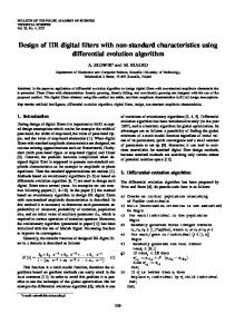
for (0,0) ≤ (i, j ) ≤ (20,20) and zero elsewhere. • The frequency weighted L2-sensitivity of the filter was found to be J 0 (Tˆ0 ) ≈ 8.60 × 103 (with Tˆ0 = I 4 ⊕ I 4 ). • With an initial Tˆ = I 4 ⊕ I 4 and tolerance ε = 10−8 , it took the algorithm 54 iterations to converge to a solution. 13

9000

8000

o

k

J (x )

7000

6000

5000

4000 0

10

20

30 k

14

40

50

• The optimized Tˆ was found to be ⎡ 3.056671 −2.673365 0.575882 −0.429287 ⎤ ⎢ −0.331629 2.142411 −0.401503 −0.192081⎥ ⎥ Tˆ opt = ⎢ ⎢ −2.530651 0.932586 0.553002 −0.136935 ⎥ ⎢ ⎥ 1.754363 − 0.312582 0.624509 0.515370 ⎣ ⎦ ⎡ 1.307170 −0.419919 0.045538 −0.194118⎤ ⎢ 0.762443 0.830435 −0.297531 0.062104 ⎥ ⎥ ⊕⎢ ⎢ −0.405202 0.189220 0.976564 −0.250656 ⎥ ⎢ ⎥ 1.071478 − 0.069804 0.315533 0.828727 ⎣ ⎦

• The minimized frequency weighted L2-sensitivity was found to be J 0 (Tˆ opt ) ≈ 4.67 ×103 .

15