1
Two-End Unsynchronized Fault Location Algorithm for Double-Circuit Series Compensated Lines Marek Fulczyk, Member, IEEE, Przemyslaw Balcerek , Jan Izykowski, Senior Member, IEEE, Eugeniusz Rosolowski, Senior Member, IEEE, Murari Mohan Saha, Senior Member IEEE
Abstract—This paper presents an accurate fault location algorithm for double-circuit series compensated lines. Use of two-end current and voltage signals with taken into account a more general case of unsynchronized measurements is studied. Different options for analytical synchronization of the measurements are considered. The algorithm applies two subroutines, designated for locating faults on particular line sections, and the procedure for selecting the valid subroutine. The subroutines are formulated with use of the generalized fault loop model, leading to compact formulae. Taking into account the distributed parameter line model assures high accuracy of fault location. Application of the proposed selection procedure allows for reliable selection of the valid subroutine. The developed fault location algorithm has been thoroughly tested using signals taken from ATP-EMTP versatile simulations of faults on a double-circuit series compensated transmission line. The presented fault location example shows the validity of the derived fault location algorithm and its high accuracy. Index Terms—ATP-EMTP, double-circuit line, fault location, series compensation, simulation, two-end unsynchronized measurement.
A
I. INTRODUCTION
CCURATE location of faults on overhead power lines for an inspection-repair purpose [1]–[2] is of vital importance for expediting service restoration, thus to reduce outage time, operating costs and customer complaints. Assuring high accuracy of fault location on series compensated lines [3]– [11] is especially important since such lines are usually spreading over few hundreds of kilometers and are vital links between the energy production and consumption centers. Different fault location algorithms for series compensated lines have been developed so far. They apply one-end [3]–[8] and two-end measurements [9]–[10] for two-terminal lines, or three-end measurements [11] for teed networks. In particular, impedance-based approach [3]–[10] is the mostly utilized J. Izykowski and E. Rosolowski are with the Wroclaw University of Technology, Wroclaw 50-370, Poland (e-mail:
[email protected];
[email protected]). M. Fulczyk and P. Balcerek are with ABB Corporate Research Center in Krakow, Poland (e-mail:
[email protected],
[email protected]). M. M. Saha is with ABB, Västeras SE-721 59, Sweden (e-mail:
[email protected]).
©2008 IEEE.
one. In [6] application of artificial neural networks combined with the impedance-based approach to fault location has been presented. Use of artificial neural networks combined with discrete wavelet transform for fault location on thyristor controlled series compensated lines has been considered [7]. In turn, [11] presents different options for traveling waves method for locating faults on teed circuits with mutually coupled lines and series capacitors. This paper presents a new fault location algorithm for double-circuit series compensated lines, with using two-end unsynchronized measurements. As so far, fault location techniques dealing with series compensation and coupled line sections have been considered for example in [8] and [11]. In particular, in [8] the one-end impedance-based approach, while in [11] the traveling waves method, have been introduced. Use of two-end measurements is assumed in this paper, with the aim of improving fault location accuracy, in comparison to the case of utilizing only one-end measurements [8]. Digital measurements can be acquired at two line ends synchronously – with use of the Global Positioning System (GPS) [10], [12], or asynchronously [9], [13], [14]. A more general case of asynchronous two-end measurements has been taken into the considerations of this paper. The presented fault location algorithm is designated for application to a line compensated with one three-phase compensating bank of fixed series capacitors (Fig. 1). The algorithm also suits thyristor controlled series compensated lines; under the condition that only one bank is applied. For the compensating banks in both parallel lines (Fig. 1) only SCs and their MOVs (applied for overvoltage protection) are shown, without the other details, as for example the thermal protection of MOVs [3]. It is considered in Fig. 1 that the fault locator (FL) is installed at the line terminal AA and is supplied with signals from the faulted line AA–BA and the healthy line AB–BB. The signals from the voltage and current instrument transformers: VTsA, CTsAA, CTsAB supply directly the fault locator. In turn, the signals from the instrument transformers at the remote end: VTsB, CTsBA, CTsBB are recorded with use of the digital fault recorder (DFR) and sent via the communication channel to the fault locator. Besides complete three-phase currents from the healthy line ends, availability of only zero-sequence currents of the healthy line
2 is considered. AB CTsAB
SCs
The three-phase SC&MOV bank divides the line of the length l [km] into two line segments having the length: d SC
CTsBB BB
System A
System B
~
FA CTsAA
MOVs SCs
~
FB CTsBA
BA
AA VTsA
FL
MOVs
DFR
VTsB
Fig. 1. Schematic diagram of two-end location of faults on double-circuit series compensated line.
It is considered that there is no GPS control of digital measurements performed at the line ends, and thus, a more general case of unsynchronized measurements, similarly as in [9] but for a single line, is taken into consideration. This differs from the approach from [10] where two-end synchronized measurements are utilized. In both [9] and [10] the distance to fault on the single line is determined by scanning along the whole faulted line section for finding the position, at which the calculated voltage and current at the fault are in phase. In order to make the fault location calculations simpler, an analytic formula for the distance to fault, with considering the distributed parameter line model, is derived in this paper. The derived algorithm is designated for locating faults on doublecircuit series compensated line, while in [9] and [10] the single-circuit line case was considered. The other aim of this study is related with analytical synchronization of the measurements. Besides considering the synchronization with use of pre-fault quantities – analogously as in [9] was applied for the single-circuit line, the other options are considered. These other options are based on processing fault quantities, and thus can be taken for an alternative use, especially since in some circumstances the registered pre-fault quantities can be considered as unreliable data or due to some reasons they are not registered at all. Fully transposed lines are taken into considerations, which allows for utilizing symmetrical components theory, without using simplifying assumptions. However, in the case of untransposed lines the phase co-ordinates approach [3] has to be applied. II. FAULT LOCATION ALGORITHM A. Basics of fault location algorithm A fault is of a random nature, and thus can appear at any line section. Thus, one has to consider a fault FA – occurring between the terminal AA and the compensating bank (Fig. 2), and also a fault FB – between the terminal BA and the bank (Fig. 3). Therefore, two subroutines: SUB_A, SUB_B are utilized for locating these hypothetical faults: FA and FB. The final result, which has to be consistent with the actual fault, is selected with use of the proposed multi-criteria selection procedure.
[p.u.] and (1 − dSC ) [p.u.]. First, the applied subroutines SUB_A, SUB_B determine the per unit distance to fault: dFA (Fig. 2) and dFB (Fig. 3), each related to the length of the particular line segment ( d SC l ) and (1 − dSC )l , both in [km]. Then, these relative distances: dFA, dFB are recalculated to the distances: dA, dB, which are related to the common basis, i.e. to the whole line length l [km]. Since use of unsynchronized measurements is considered in this study, the common phase reference for the phasors from two line ends has to be assured. This is performed by assuming the measurements from one line end as the basis, while the measurements from the other end undergo an analytical synchronization. This synchronization in case of the subroutine SUB_A (Fig. 2) is accomplished by multiplying the phasors from the end AA–AB by the synchronization operator: exp(jδΑ), while in case of the subroutine SUB_B (Fig. 3) –multiplying the phasors from the end BA–BB by the synchronization operator: exp(jδΒ).
AB I ABi e
BB C
jδ A
MOV FA
V SUB_A Vi
I AAi e jδA
AA
I BBi
I BAi
C transf. I BAi
MOV
V Ai e jδA
BA
transf. I BAi
V Bi
dFA [p.u.] (1–dFA) [p.u.] (1 − dSC ) [p.u.]
dSC [p.u.]
Fig. 2. Scheme of double-circuit series compensated line for ith symmetrical component under fault FA, located with subroutine SUB_A.
AB
BB C
I ABi
FB
V SUB_B Vi
I AAi
AA
I BBi e jδB
MOV
I BAi e jδB
C transf.
I AAi
MOV
V Bi e jδB
V Ai (1–dFB) [p.u.] dSC [p.u.]
BA
I transf. AAi
dFB [p.u.]
(1 − d SC ) [p.u.]
Fig. 3. Scheme of double-circuit series compensated line for ith symmetrical component under fault FB, located with subroutine SUB_B.
B. Fault location subroutines The schemes of the faulted double-circuit series compen-
3 sated lines for the ith symmetrical component, utilized in the derivation of the subroutines, are shown in Fig. 2 (for the subroutine SUB_A) and Fig. 3 (for the subroutine SUB_B). The index i is applied for denoting a type of the symmetrical component of current or voltage signal: i=1–positive-, i=2– negative-, i=0–zero-sequence signal, respectively. This index is also applied for denoting the impedance parameters of the line. On the other hand, the positive- and negative-sequence parameters for overhead lines are identical. Therefore, there is no need to distinguish such identical impedances and the subscript 1 (as for positive-sequence) is uniformly applied for both the positive- and negative-sequence parameters: characteristic impedance and propagation constant of the line. Both the subroutines of the fault location algorithm are based on the same principle and only one of them: the subroutine SUB_A is derived here. The latter subroutine SUB_B can be derived analogously to the presented SUB_A. The line segment adjacent to the bus BA (Fig. 2) is healthy and thus one can transfer analytically the current ( I BAi ) along the whole segment, i.e. from the bus BA towards the SC&MOV bank, obtaining: I transf. BAi =
− V Bi sinh( γ (1 − d SC )l) + cosh(γ (1 − dSC )l) ⋅ I BAi (1) i i Z ci
where Z ci – characteristic impedance of the line, γ – propagation i constant, both for the ith sequence. Taking the transferred current (1), which flows at both sides of the compensating bank (Fig. 2), together with the voltage ( V Ai ) and current ( I AAi ) from the bus AA, we get incomplete two-end measurements for locating faults on the faulted line segment adjacent to the bus AA. This is so since the voltage from the bus BA cannot be transferred analytically beyond the bank without knowing the voltage drop across it. Due to having the incomplete two-end measurements for the considered line segment, the natural fault loops have to be considered, instead of processing the individual symmetrical components type. Accordingly to the identified fault type, the single-phase loop (for phase-to-ground faults) or inter-phase loop (for faults involving two or three phases) has to be considered. The fault loop contains the section of the line from the measuring point up to the fault spot and also the fault path resistance. The generalized fault loop model [15] is applied for determining the distance to fault: V FAp (d FA ) − RFA I FA = 0 (2) where V FAp (d FA ) – fault loop voltage after transferring from the bus A to the fault point FA, d FA – distance from the bus AA to the fault FA (p.u.), RFA – fault path resistance, I FA – fault path current (total fault current).
The voltage at the fault point FA, for the considered fault loop, can be composed as the weighted sum of the respective
sequence components [15]: V FAp (d FA ) = a1V FA1 (d FA ) + a 2 V FA2 (d FA ) + a 0 V FA0 (d FA ) (3) where V FA1 = [V A1 cosh(γ dSC ld FA ) − Z c1 I AA1 sinh(γ 1d SC ld FA )]e jδA 1 V FA2 = [V A2 cosh(γ d SC ld FA ) − Z c1 I AA2 sinh( γ d SC ld FA )]e jδA 1
1
V FA0 = [V A0 cosh( γ 0 d SC ld FA ) − Z c0 I AA0 sinh( γ 0 d SC ld FA ) − dSC ld FA Z '0m I AB0 ]e jδA
a 1 , a 2 , a 0 – weighting coefficients gathered in Table I, Z '0m – zero-sequence mutual coupling impedance [Ω/km]. When calculating the zero-sequence component of voltage at the fault (VFA0), involved in (3), the voltage drop on the faulted line section due to the flow of its zero-sequence current (IAA0), as well as the voltage induced due to the flow of the zero-sequence current (IAB0) in the healthy parallel line (the mutual coupling effect) are taken into account. TABLE I WEIGHTING COEFFICIENTS USED FOR COMPOSING FAULT LOOP VOLTAGE (3).
FAULT a-g b-g
a1
a2
a0
1
1 a
1
2
1
a
2
1
c-g
a
a
a-b, a-b-g a-b-c, a-b-c-g
1 – a2
1– a
0
b-c, b-c-g
a2 − a
a − a2
0
c-a, c-a-g
a −1
a 2 −1
0
a = exp( j2 π / 3) ; j = − 1
In [15] it has been introduced that the total fault current ( I FA ) can be expressed as the following weighted sum of its symmetrical components ( I FA1 , I FA2 , I FA0 ): I FA = a F1 I FA1 + a F2 I FA2 + a F0 I FA0 (4) where a F1 , a F2 , a F0 – share coefficients, dependent on fault type
and the assumed preference for using particular components. There is a possibility of applying different, alternative sets of share coefficients [15], however, the coefficients for which the zero-sequence is eliminated ( a F0 = 0 ), as in Table II, is recommended for the considered application. The symmetrical components of the total fault current involved in (4) can be simply determined by summing the respective components of the currents from the ends of the considered line segment (Fig. 2): transf. I FAi = I AAi e jδ A + I BA (5) i However, more accurate determination is achieved with strict taking into account the distributed parameter line model for the considered faulted line segment (for the considered subroutine SUB_A: from the bus AA to the compensating
4 bank).
bolic trigonometric function under the consideration. TABLE II RECOMMENDED SET OF SHARE COEFFICIENTS FOR DETERMINING TOTAL FAULT CURRENT.
FAULT a–g b–g
a F1 0 0
a F2 3 3a
a F0 0 0
c–g
0
3a 2
0
a–b
0
1− a
0
b–c
0
a − a2
0
c-a
2
0 2
0
jδ A I pre AA1e
AA
a2 − a
a − a2
0
a −1
a2 −1
0
1− a
I pre_transf e jδ A AB1
1− a
b-c-g
a-b-c, a-b-c-g
BB
1− a
*)
0
Taking the currents from both ends of the faulted line segment and the voltage at its beginning, after detailed consideration of the flow of currents one derives (see: APPENDIX I): Mi (6) I FAi = cosh(γ i d SC l(1 − d FA )) where Mi = transf.
I BAi
transf. I BAi
V + [ I AA1 cosh(γ i dSC l) − Ai sinh( γ i d SC l)]e jδ A Z ci
– current transferred analytically according to (1).
Taking into account (4) and (6), together with the share coefficients from Table II, allows to present the fault loop model (2) in the following compact form: 2 2 a Fi M i a i V FAi (d FA ) − RFA =0 (7) cosh( γ d l(1 − d FA )) i =0 i =1 1 SC
∑
∑
where V FAi (d FA ) – fault loop voltage at the fault point, as in (3), M i – quantity defined in (6), a i , a Fi – coefficients dependent on fault type: Table I and II.
Determining earlier the synchronization operator exp(jδΑ), which is involved in both quantities: V FAi (d FA ) and M i , the formula (7) becomes as in two unknowns: distance to fault dFA and fault resistance RFA. Solution for these unknowns can be obtained after resolving (7) into the real and imaginary parts, and applying one of the numeric procedures for solving nonlinear equations. It has been checked that the Newton-Raphson iterative method is a good choice for that. In case of such choice, the start of iterative calculations can be performed with the initial values for the unknowns calculated from the linear form of (7) – obtained by introducing the substitutions: cosh(x) 1, sinh(x) x, where x is the argument of the hyper-
pre
I BB1
MOV
pre_transf.
I BB1
I pre BA1
C . jδ A I pre_transf e AA1
MOV
. I pre_transf BA1
jδ A V pre A1 e
BA V pre B1
dSC [p.u.]
*)
– there is no negative sequence component under these faults and the coefficient can be assumed as equal to zero
C
jδ A I pre AB1e
0
1− a
2
AB
a −1
a-b-g
c-a-g
C. Synchronization of measurements 1) Synchronization with use of pre-fault measurements Analogously, as in [9] for the single-circuit line, the synchronization utilizing the pre-fault positive-sequence measurements can be applied for double-circuit series compensated line (Fig. 4).
(1–dSC) [p.u.]
Fig. 4. Scheme of double-circuit series compensated line for pre-fault positive-sequence.
Applying the distributed parameter line model for transferring currents from the buses AA and BA towards the compensating bank (analogously as in (1)), one gets the currents: . jδ A . I pre_transf e , I pre_transf . These currents have identical magAA1 BA1 nitudes but opposite signs, and thus:
e jδ A =
. − I pre_transf BA1
(8)
. I pre_transf AA1
The synchronization operator used in the subroutine SUB_B (Fig. 3) is determined as: e jδ B = −e jδ A (9) Analogously, instead of signals from the line AA–BA (8) one can utilize the pre-fault signals from the parallel line AB– BB for determining the synchronization operator. Use of pre-fault quantities in some circumstances is troublesome, therefore the other ways are considered further. 2) Synchronization with use of fault quantities from healthy parallel line Fig. 5 depicts use of positive-sequence quantities from healthy parallel line AB–BB for the synchronization.
AB
jδ A I transf AB1 e
transf.
I BB1 C
I AB1e jδ A
BB I BB1
MOV FA C
AA
BA
MOV V A1e jδ A
V B1 dSC [p.u.]
(1–dSC) [p.u.]
5 Fig. 5. Scheme of double-circuit positive-sequence under fault FA.
series
compensated
line
for
If the three-phase currents at both ends of the healthy line AB–BB are available as the inputs of the fault locator, then one can consider the flow of the positive-sequence currents in this line during the fault period for deriving the synchronization procedure. It is analogous to that based on pre-fault measurements – presented in (8)–(9). When adapting the formulae (8)–(9), one has to delete ‘pre_’ in the superscripts and in the subscripts the indexes relevant for the healthy parallel line (AB, BB) have to be inserted in place of the indexes (AA, BA) for the faulted line. In case, if only zero-sequence currents from both ends of the healthy line are available, then the synchronization, as presented in the next paragraph, has to be applied. This is so since the zero-sequence line parameters are considered as unreliable data, and thus their usage, if possible, has to be avoided. 3) Synchronization with use of fault quantities from faulted line The other option for performing the synchronization for the subroutine SUB_A (analogously is for the subroutine SUB_B) is based on utilizing an information brought by the fault boundary conditions and processing the fault quantities from the faulted line. This can be accomplished for phase-toground and phase-to-phase faults. For the remaining fault types, the synchronization with use of positive-sequence fault quantities from the healthy parallel line (paragraph 2 of the Section C) or according to (8)–(9) with use of the pre-fault quantities remains. As for example for a-g fault of the fault FA (Fig. 2) there is a non zero current in phase ‘a’, while no flow in the remaining phases ‘b’ and ‘c’ at the fault place: I FAa ≠ 0 and I FAb = I FAc = 0 (10) and thus the symmetrical components of the total fault current: I (11) I FA1 = I FA2 = I FA0 = FAa . 3 The total fault current flowing in phase ‘a’ can be expressed alternatively as: I FAa = 3I FA1 or I FAa = 3I FA2 (12) Similarly, for the other fault types from the category of phase-to-ground (ph-g) and phase-to-phase (ph1-ph2) faults, two characteristic sets (among the other possible) of the share coefficients are obtained, as gathered in Table III. Applying the I-SET from Table III (positive- and zero-sequence are eliminated), the total fault current for the subroutine SUB_A becomes: I FA = a IF2– SET I FA2 (13) or alternatively with use of the II-SET (negative- and zerosequence are eliminated): a IIF1– SET I FA1
I FA = (14) Substituting (6) into (13)–(14), after taking into account that the line propagation constants are identical for both the
positive- and negative-sequence ( γ = γ ), one gets the fol1
2
lowing compact formula for the synchronization operator: [e jδ A ](ph – g) or (ph1– ph2) =
II – SET transf. a IF–2SET I transf. I BA1 BA2 − a F1
a IIF1–SET M 1 − a IF2–SET M 2
(15)
where transf. transf. I BA1 , I BA2 – calculated as in (1);
M 1 , M 2 – quantities defined in (6); a IF2– SET , a IIF1– SET – coefficients from Table III. TABLE III TWO ALTERNATIVE SETS OF SHARE COEFFICIENTS FOR PHASE-TO-GROUND FAULTS AND PHASE-TO-PHASE FAULTS.
I–SET FAULT a I – SET F1 a–g
0
II–SET
a IF–2SET
a IF0– SET
a IIF1– SET
3
0
3 2
a IIF 2– SET a IIF0– SET
0
0
0
0
b–g
0
3a
0
3a
c–g
0
3a 2
0
3a
0
0
a–b
0
1− a
0
1− a2
0
0
b–c
0
a − a2
0
a2 − a
0
0
c-a
0
a2 −1
0
a −1
0
0
Thus, the synchronization operator in (15), applicable for phase-to-ground and phase-to-phase faults, is determined with processing signals from the fault period, and not from the prefault interval, as in (8).
D. Selection procedure The applied two subroutines SUB_A, SUB_B yield the results for a distance to fault and fault resistance: (dFA, RFA), (dFB, RFB), respectively. The results from only one subroutine are consistent with the actual fault, and thus there is a need for selecting such valid subroutine. First, the subroutine yielding the distance to fault outside the section range and/or the fault resistance of negative value is rejected. Next, the estimated equivalent impedance of the series capacitor and its MOV, in terms of the impedance for the phase involved in a fault, is determined for both subroutines. The way of estimation of this equivalent impedance is further presented in relation to the subroutine SUB_A, while for the subroutine SUB_B is entirely analogous. For the subroutine SUB_A the equivalent impedance is deSUB_A termined with the calculated signals: I transf. (Fig. 2): BAi , V Vi
Z SUB_A V
=
f 1V SUB_A + f 2 V SUB_A + f 0 V SUB_A V0 V2 V1 transf. transf. transf. f 1 I BA 1 + f 2 I BA2 + f 0 I BA0
(16)
where V SUB_A – ith symmetrical component of voltage drop Vi across the compensating bank, I transf. – ith symmetrical component of transferred current BAi
6 (1), f i – coefficients allowing to compose the voltage and current in the first phase involved in the fault (Table IV). The voltage drop across the compensating bank for the subroutine SUB_A can be calculated as the difference of voltages at its both sides, determined for the lumped line model: V
SUB_A Vi
=V
SUB_A VBi
−V
SUB_A VAi
SUB_A
= V Bi − (1 − d SC )lZ 1L I BAi '
(18)
V SUB_A = [V Ai − dSCld FA Z 1' L I AAi ]e jδ A + dSCl(1 − d FA ) Z 1' L I BAi VAi
where Z 1' L
(19)
– positive- (negative-) sequence line impedance [Ω/km].
In case of the zero-sequence, the mutual coupling effect along the whole line length is additionally taken into account obtaining: SUB_A
V V0
SUB_A
= V VB0
SUB_A
− V VA 0
− lZ 0' m I BB0
(20)
where SUB_A
V VB0
= V B0 − (1 − d SC )l Z 0 L I BA 0
V SUB_A VA 0
= [V A 0 − dSCld FA Z '0L I AA 0 ]e jδ A
'
(21) + dSCl(1 − d FA ) Z '0 L I BA0
where Z '0 L
FAULT a-g, a-b, a-b-g, a-b-c, a-b-c-g
f1
f2
f0
1
1 a
1
a2
1
2
b-g, b-c, b-c-g
a
c-g, c-a, c-a-g
a
(17)
For the positive- and negative-sequence (i=1 and i=2) the voltage drop (17) is determined using: V VBi
TABLE IV COEFFICIENTS FOR COMPOSING PHASE QUANTITIES INVOLVED IN (16).
(22)
– zero-sequence line impedance [Ω/km].
Taking into account (17)–(22) and Table IV, the equivalent impedance Z SUB_A of the series capacitor and its MOV for V the subroutine SUB_A is determined according to (16), utilizing the earlier calculated distance to fault: dFA, and the synchronization operator: exp(jδA). Analogously, the equivalent impedance Z SUB_B for the subroutine SUB_B is determined. V The real, imaginary parts or the angle of the equivalent impedances: Z SUB_A , Z SUB_B , estimated according to both subV V routines, are analyzed for selecting the valid subroutine. The equivalent impedance for the valid subroutine has to be of the R–C character, i.e. with the positive real part and the negative imaginary part [9]–[10]. Since the compensation degree is the highest for the normal load conditions (MOVs conduct very low currents), also the imaginary part of the equivalent impedance has to be smaller than the reactance of the compensating capacitor.
1
III. ATP-EMTP EVALUATION The 300 km, 400 kV double-circuit transmission line compensated in the middle (dSC=0.5 p.u.), at the degree of 70%, was modeled using ATP-EMTP [16]. The line impedances were assumed as: Z1'L = (0.0276 + j0.3151) Ω/km , Z 0' L = (0.275 + j1.0265) Ω/km , Z 0' m = (0.21 + j 0.6283) Ω/km , line capacitances: C1L=13 nF/km, C0L=8.5 nF/km, C0m=5 nF/km. The supplying systems were modeled with impedances: Z1SA=Z1SB=(1.31+j15)Ω, Z0SA=Z0SB=(2.32+j26.5)Ω; the E.M.F. of the system B delayed by 30o with respect to the equivalent system A. The MOVs with the common approximation: v q i = P( ) (23) VREF
were modeled taking: P=1 kA, VREF=150 kV, q=23. The developed ATP-EMTP model includes the Capacitive Voltage Transformers (CVTs) and the Current Transformers (CTs). The analogue filters with 350 Hz cut-off frequency were also included. The sampling frequency of 1000 Hz was applied and the phasors were determined with use of the DFT algorithm. Fig. 6–Fig. 8 present the results for the example fault: • fault type: a-g; • fault distance: dA=0.5– p.u. (just in front of the compensating bank, as seen from the bus AA); • fault resistance: RFA=10 Ω; • phasors of voltage and current from the remote line end B were delayed by 18o with respect to the line side A phasors.
7
SIDE A – Voltages: vA [105 V]
a b c 3 2 1 0 -1
4000
SIDE A – Currents of healthy line: iAB [A]
SIDE A – Currents of faulted line: iAA [A]
4
3000 2000 a b c 1000 0
-4 0
20
40
60 Time [ms]
80
100
120
1000 0
-2000
-2000
-3
2000 a b c
-1000
-1000
-2
3000
-3000 0
20
40
60 Time [ms]
80
100
120
-3000 0
20
40
60 Time [ms]
80
100
120
Fig. 6. The fault location example: waveforms of voltage and current signals from the side A. a b c
3 2 1 0
-1
3000 2000
a b c
1000 0
-1000
-2
40
60 Time [ms]
80
100
120
-4000 0
2000 1000 0
-2000 a b c
-3000
20
3000
-1000
-2000
-3 -4 0
4000
SIDE B – Currents of healthy line: iBB [A]
SIDE B – Currents of faulted line: iBA [A]
SIDE B – Voltages: vB [105 V]
4
20
40
60 80 Time [ms]
100
120
-3000 0
20
40
60 80 Time [ms]
100
120
Fig. 7. The fault location example: waveforms of voltage and current signals from the side B.
0.6
60
SUB_A
0.4
SUB_B
RFA_(30–50)ms=9.86 Ω RFB_(30–50)ms=26.9 Ω
50 40 30
SUB_B
20
SUB_A 10
0.2
0
0
20 40 Postfault time [ms]
60
0
20 40 Postfault time [ms]
60
40 Estimated impedance of SC/MOV [Ω]
0.8
dA_(30–50)ms=0.4982 p.u. dB_(30–50)ms=0.2537 p.u.
Fault resistance [Ω]
Distance to fault [p.u.]
1
real( Z SUB_A ) V 20 imag( Z SUB_A ) V 0
-20
-40
0
SUB_B
imag( Z V
)
real( Z SUB_B ) V
20 40 Postfault time [ms]
60
Fig. 8. The fault location example: estimated distance to fault, fault resistance and impedance of SC/MOV according to subroutines SUB_A and SUB_B.
Fig. 6–Fig. 7 presents waveforms of the fault locator input signals acquired at both line sides. In Fig. 8 the estimated distance to fault and fault resistance is shown. The fault distances yielded by the subroutines: dFA, dFB are recalculated to: dA, dB, which are related to the whole line length. The fault distances of both subroutines are within the line sections and the fault resistances are of positive values. Therefore the selection has to be continued. In Fig. 8 the real/imaginary parts of the equivalent impedance for the SC&MOV from the faulted phase ‘a’ are shown. The subroutine SUB_A yields the equivalent impedance of the R–C character, which is consistent with the reality. In contrast, the subroutine SUB_B estimates the equivalent resistance being of evidently negative value. Finally, the subroutine SUB_A remains selected as the valid, giving estimation of the fault distance to fault with around 0.2% error. It has been checked that for very wide range of fault specifications
and network parameters, the fault location error basically does not exceed 0.5%. Mainly, the transformation errors of the included instrument transformers contribute to such errors since the fault location algorithm itself is very accurate. IV. CONCLUSIONS This paper presents an accurate fault location algorithm for double-circuit series compensated lines. The algorithm consists of two subroutines, designated for locating faults on the line segments at both sides of the compensating bank. Multicriteria efficient procedure for selecting the valid subroutine, which yields the results consistent with the actual fault, has been presented. The subroutines of the algorithm have been formulated with use of the generalized fault loop model, leading to the compact formulae. Taking into account the distributed parameter line model assures high accuracy of fault location.
8 The distance to fault calculation is independent on the compensating bank parameters, except the position at which the bank is installed. Use of two-end signals with a more general case of unsynchronized measurements has been considered. New synchronization procedure, which allows to avoid usage of the prefault quantities for phase-to-ground and phase-to-phase faults, thus for majority of all faults, has been developed. The developed fault location algorithm has been thoroughly tested using signals taken from ATP-EMTP versatile simulations of faults on a double-circuit series compensated transmission line. The presented fault location example shows the validity and high accuracy of the fault location algorithm and reliable selection of the valid subroutine. V. APPENDIX I – DERIVATION OF FORMULA FOR TOTAL FAULT CURRENT OF SUBROUTINE SUB_A Applying the distributed parameter model for the section AA-FA of the segment of the faulted line (there is no need for considering the flow of currents in the healthy line), as shown in Fig. 9, one transfers the signals towards the fault point FA: V FAi = V Ai cosh(γ d SC ld FA ) − Z ci I AAi sinh(γ d SC ld FA ) (A1) i i transf.
I AAi = −
V Ai
sinh( γ i d SC l d FA ) + I A1 cosh( γ i d SC ld FA ) (A2) Z ci Transferring the current (A2) along the line section FA-SC/MOV towards the compensating bank, one obtains: transf.
I BAi =
jδA
V FAi e sinh( γ i d SC l (1 − d FA )) Z ci transf. jδA − ( I AA − I FAi ) cosh( γ d SC l (1 − d FA )) i e
[2] [3] [4] [5] [6]
[7]
[8] [9]
[10] [11] [12] [13]
(A3)
[14]
A
i
A
δ
I AAi e j
AA
j I transf. AAi e
δ
I FAi
transf.
I BAi
V FAi e jδ A
FA
[15]
SC/ MOV
V Ai e jδ A
I FAi
I
[16]
VII. BIOGRAPHIES II
Fig. 9. Segment of faulted line considered for deriving total fault current for ith sequence under fault FA (subroutine SUB_A): I–long line representation of the section having length [ d SCld FA ]; II–long line representation of the section having length [ d SCl(1 − d FA ) ].
Substituting signals (A1)–(A2) into (A3), after tedious rearrangements – performed with applying the identities: sinh( x + y ) = sinh( x) cosh( y ) + cosh( x) sinh( y ) (A4) cosh( x + y ) = sinh( x) sinh( y ) + cosh( x) cosh( y ) (A5) one gets the ith sequence of the total fault current as in (6).
VI. REFERENCES [1]
IEEE Std C37.114: “IEEE Guide for Determining Fault Location on AC Transmission and Distribution Lines”, IEEE Power Engineering Society Publ., pp. 1-42, 8 June 2005. M. M. Saha, J. Izykowski, E. Rosolowski, B. Kasztenny, “A new accurate fault locating algorithm for series compensated lines”, IEEE Trans. Power Del., Vol. 14, No. 3, pp. 789–797, 1999. Sadeh, N. Hadjsaid, A. M. Ranjbar, R. Feuillet, “Accurate fault location algorithm for series compensated transmission lines”, IEEE Trans. Power Del., Vol. 15, No. 3, pp.1027–1033, 2000. E. Rosolowski, J. Izykowski, M. M. Saha, “Differential equation based fault location algorithm for series-compensated transmission line”, CD Proceedings of Power Systems Computation Conference, Liege, 2005. D. Novosel, B. Bachmann, D. Hart, Y. Hu, M. M. Saha, “Algorithms for locating faults on series compensated lines using neural network and deterministic methods”, IEEE Trans. Power Del., Vol. 11, No. 4, pp. 1728– 1736, 1996. W. J. Cheong, R. K. Aggarwal, “A novel fault location technique based on current signals only for thyristor controlled series compensated transmission lines using wavelet analysis and self organising map neural networks”, Proceedings of 8-th IEE International Conference on Developments in Power System Protection, Vol. 1, pp. 224–227, 2004. M. M. Saha, K. Wikström, J. Izykowski, E. Rosolowski, “Fault location in uncompensated and series-compensated parallel lines”, CD Proceedings of 2000 IEEE PES Winter Meeting, Singapore, 6 p., 23-27 January 2000. C. Fecteau, “Accurate fault location algorithm for series compensated lines using two-terminal unsynchronised measurements and Hydro-Quebec’s field experience”, Proceedings of 33rd Annual Western Protective Relay Conference, Spokane, Washington, pp. 1–16, 2006. C.-S. Yu, C.-W. Liu, S.-L. Yu, J.-A. Jiang, “A new PMU-based fault location algorithm for series compensated lines”, IEEE Trans. Power Del., Vol. 17, No. 1, pp. 33–46, 2002. C. Y. Evrenosoglu, A. Abur, “Fault location for teed circuits with mutually coupled lines and series capacitors”, Proceedings of IEEE Bologna Power Tech Conference, IEEE Catalog Number 03EX719C, 2003. IEEE Std. C37.118: “IEEE Standard for Synchrophasors for Power Systems”, IEEE Power Engineering Society Publ., pp. 1-65, 22 March 2006. Y. Liao, M. Kezunovic, “Optimal estimate of transmission line fault location considering measurement errors”, IEEE Trans. Power Del., Vol. 22, No.3, pp. 1335–1341, 2007. Y. Liao, S. Elangovan, “Unsynchronised two-terminal transmission-line fault-location without using line parameters”, IEE Proc.-Gener. Transm. Distrib., Vol. 153, No. 6, pp. 639–643, 2006. J. Izykowski, E. Rosolowski, M. M. Saha, “Locating faults in parallel transmission lines under availability of complete measurements at one end”, IEE Proc.-Gener. Transm. Distrib., Vol. 151, No. 2, pp. 268–273, 2004. H. W. Dommel, Electro-Magnetic Transients Program, BPA, Portland, Oregon, 1986.
M. S. Sachdev (coordinator), “Advancements in microprocessor based protection and communication”, IEEE Tutorial, Publ. No. 97TP120–0, 1997.
Marek Fulczyk (M’04) was born in 1968 in Poland. He received the M.Sc. and Ph.D. degrees in electrical engineering from the Wroclaw University of Technology, Wroclaw, Poland, in 1993 and 1997, respectively. In 1997 he joined ABB as a research scientist. Now he is a group leader of Electrical & Engineering Systems at ABB Corporate Research Center in Krakow, Poland. His fields of interests include power system protection, power system/voltage stability, real-time collaborative technology, 3D modeling and simulations of phenomena in power systems. Przemyslaw Balcerek was born in 1976 in Poland. He received his M.Sc. and Ph.D. degrees in electrical engineering from the Wroclaw University of Technology, Wroclaw, Poland, in 2000, 2004 respectively. Fault location, instrument transformers and ATP-EMTP simulation of power system transients are in the scope of his research interests. Presently he is with ABB Corporate Research Center in Krakow, Poland, as a research scientist.
9 Jan Izykowski (M’97–SM’04) was born in 1949 in Poland. He received his M.Sc., Ph.D. and D.Sc. degrees from the Faculty of Electrical Engineering of Wroclaw University of Technology (WUT), Wroclaw, Poland, in 1973, 1976 and in 2001, respectively. In 1973 he joined Institute of Electrical Engineering of the WUT, where presently he is an Associate Professor. His research interests are in power system transients simulation, power system protection and control, and fault location. Eugeniusz Rosolowski (M’1997–SM’00) was born in 1947 in Poland. He received his M.Sc. degree in electrical engineering from the Wroclaw University of Technology (WUT), Wroclaw, Poland, in 1972. From 1974 to 1977, he studied in Kiev Politechnical Institute, Kiev, Ukraine, where he received Ph.D. in 1978. In 1993 he received D.Sc. from the WUT. Presently he is a Professor in the Institute of Electrical Engineering. His research interests are in power system analysis and microprocessor applications in power systems.
Murari Mohan Saha (M´76–SM´87) was born in 1947 in Bangladesh. He received B.Sc.E.E. and M.Sc.E.E. from Bangladesh University of Engineering and Technology (BUET), Dhaka, Bangladesh, in 1968 and 1970 respectively. In 1975 he received Ph.D. from the Technical University of Warsaw, Poland. Currently he is a Senior Research and Development Engineer at ABB AB, Västerås, Sweden. His areas of interest are power system simulation, instrument transformers and digital protective relays.