Nov 26, 2014 - ... operators, the weight function for the polynomials Jn,k(x, y) will be recovered. arXiv:1411.7299v1 [math.CA] 26 Nov 2014 ...
Two-variable −1 Jacobi polynomials Vincent X. Genest1 , Jean-Michel Lemay1 , Luc Vinet1 , and Alexei Zhedanov2
arXiv:1411.7299v1 [math.CA] 26 Nov 2014
1
Centre de recherches mathématiques, Université de Montréal, P.O. Box 6128, Centre-ville Station, Montréal, Canada, H3C 3J7 2 Donetsk Institute for Physics and Technology, Donetsk 340114, Ukraine
Abstract A two-variable generalization of the Big −1 Jacobi polynomials is introduced and characterized. These bivariate polynomials are constructed as a coupled product of two univariate Big −1 Jacobi polynomials. Their orthogonality measure is obtained. Their bispectral properties (eigenvalue equations and recurrence relations) are determined through a limiting process from the twovariable Big q-Jacobi polynomials of Lewanowicz and Wo´zny. An alternative derivation of the weight function using Pearson-type equations is presented. Keywords: Bivariate Orthogonal Polynomials, Big −1 Jacobi polynomials AMS classification numbers: 33C50
1
Introduction
The purpose of this paper is to introduce and study a family of bivariate Big −1 Jacobi polynomials. These two-variable polynomials, which shall be denoted by Jn,k (x, y), depend on four real parameters α, β, γ, δ such that α, β, γ > −1, δ 6= 1 and are defined as µ ¶ ³ ´ δ x , (1) Jn,k (x, y) = Jn−k y; α, 2k + β + γ + 1, (−1)k δ ρ k (y) Jk ; γ, β, y y with k = 0, 1, . . . and n = k, k + 1, . . ., where ³ ´k yk 1 − δ22 2 , k even, y ρ k (y) = k−1 ³ ³ ´ ´ yk 1 − δ2 2 1 + δ , k odd, y y2 and where Jn (x; a, b, c) denotes the one-variable Big −1 Jacobi polynomials [20] (see section 1.1). It will be shown that these polynomials are orthogonal with respect to a positive measure defined on the disjoint union of four triangular domains in the real plane. The polynomials Jn,k (x, y) will also be identified as a q → −1 limit of the two-variable Big q-Jacobi polynomials introduced by Lewanowicz and Wo´zny in [16], which generalize the bivariate little q-Jacobi polynomials introduced by Dunkl in [3]. The bispectral properties of the Big −1 Jacobi polynomials will be determined from this identification. The polynomials Jn,k (x, y) will be shown to satisfy an explicit vector-type three term recurrence relation and it will be seen that they are the joint eigenfunctions of a pair of commuting first order differential operators involving reflections. By solving the Pearson-type system of equations arising from the symmetrization of these differential/difference operators, the weight function for the polynomials Jn,k (x, y) will be recovered.
The defining formula of the two-variable Big −1 Jacobi polynomials (1) is reminiscent of the expressions found in [15] for the Krall-Sheffer polynomials [14], which, as shown in [11], are directly related to two-dimensional superintegrable systems on spaces with constants curvature (see [17] for a review of superintegrable systems). The polynomials Jn,k (x, y) do not belong to the Krall-Sheffer classification, as they will be seen to obey first order differential equations with reflections. The results of [11] however suggest that the polynomials Jn,k (x, y) could be related to two-dimensional integrable systems with reflections such as the ones recently considered in [5, 7, 6, 9]. This fact motivates our examination of the polynomials Jn,k (x, y).
1.1
The Big −1 Jacobi polynomials
Let us now review some of the properties of the Big −1 Jacobi polynomials which shall be needed in the following. The Big −1 Jacobi polynomials, denoted by Jn (x; a, b, c), were introduced in [20] as a q = −1 limit of the Big q-Jacobi polynomials [12]. They are part of the Bannai-Ito scheme of −1 orthogonal polynomials [10, 8, 18, 19]. They are defined by µ n n+a+b+2 ¯ ¶ µ n n+a+b+2 ¯ ¶ −2, 1− 2 , ¯ 1− x2 ¯ 1− x 2 n(1− x) 2 2 n even, ¯ 1− c2 + (1+ c)(a+1) 2 F1 ¯ 1− c2 , a+1 a+3 2 F 1 2 2 ¶ µ n−1 n+a+b+3 ¯ ¶ µ n−1 n+a+b+1 ¯ Jn (x; a, b, c) = (2) 2 2 2 F1 − 2 ,a+1 2 ¯¯ 1− x2 − (n+a+b+1)(1− x) 2 F1 − 2 ,a+3 2 ¯¯ 1− x2 , n odd, (1+ c)(a+1) 1− c 1− c 2
2
where 2 F1 is the standard Gauss hypergeometric function [1]; when no confusion can arise, we shall simply write Jn (x) instead of Jn (x; a, b, c). The polynomials (2) satisfy the recurrence relation x Jn (x) = A n Jn+1 (x) + (1 − A n − C n ) Jn (x) + C n Jn−1 (x), with coefficients ( An =
( n+a+1)( c+1) 2 n+a+ b+2 , (1− c)( n+a+ b+1) 2 n+a+ b+2 ,
n even, n odd,
(
Cn =
n(1− c) 2 n+ a+ b , ( n+ b)(1+ c) 2 n+ a+ b ,
n even, n odd.
It can be seen that for a, b > −1 and | c| 6= 1 the polynomials Jn (x) are positive-definite. The Big −1 Jacobi polynomials satisfy the eigenvalue equation © ª L Jn (x) = (−1)n (n + a/2 + b/2 + 1/2) Jn (x),
(3)
where L is the most general first-order differential operator with reflection preserving the space of polynomials of a given degree. This operator has the expression · ¸ · ¸ · ¸ (x + c)(x − 1) c ca − b a+b+1 L= ∂x R + + (R − I) + R, x 2x 2 2x2 where R is the reflection operator, i.e. R f (x) = f (− x), and I stands for the identity. The orthogonality relation of the Big −1 Jacobi polynomials is as follows. For | c| < 1, one has " # a+ b+2 Z (1 − c2 ) 2 Jn (x; a, b, c) Jm (x; a, b, c) ω(x; a, b, c) dx = h n (a, b) δnm , (4) (1 + c) C
where the interval is C = [−1, −| c|] ∪ [| c|, 1] and the weight function reads ω(x; a, b, c) = θ (x) (1 + x) (x − c) (x2 − c2 )
b−1 2
(1 − x2 ) 2
a−1 2
,
(5)
with θ (x) is the sign function. The normalization factor h n is given by ¡ ¢ 2 Γ n+2b+1 Γ( n+2a+3 )( n2 )! n even, (n+a+1) Γ¡ n+a+b+2 ¢( a+1 )2n , 2 2 2 ¡ ¢ h n (a, b) = (n+a+b+1) Γ n+b+2 Γ n+a+2 n−1 ! ( 2 )( 2 ) 2 , n odd, ¡ ¢ 2 2 Γ n+a+2 b+3 ( a+2 1 ) n+1 2 where (a)n stands for the Pochhammer symbol [1]. For | c| > 1, one has " # a+ b+2 Z θ (c)(c2 − 1) 2 e n (a, b) δnm , h Jn (x; a, b, c) Jm (x; a, b, c) ω e (x; a, b, c) dx = 1+ c
(6)
(7)
Ce
where the interval is Ce = [−| c|, −1] ∪ [1, | c|] and the weight function reads ω e (x; a, b, c) = θ (c x) (1 + x) (c − x) (c2 − x2 )
b−1 2
(x2 − 1)
a−1 2
.
In this case the normalization factor has the expression ¢ ¡ 2 Γ n+2b+1 Γ( n+2a+3 )( n2 )! n even, ¡ ¢ 2 , ( n+a+1)Γ n+a+2 b+2 ( a+2 1 ) n 2 e n (a, b) = ¢ ¡ h ( n+a+ b+1) Γ n+2b+2 Γ( n+2a+2 )( n−2 1 )! n odd. ¡ ¢ 2 2 Γ n+a+2 b+3 ( a+2 1 ) n+1 2
(8)
(9)
e n were not derived in [20]. They have been obtained here using The normalization factors h n and h the orthogonality relation for the Chihara polynomials provided in [8] and the fact that the Big −1 Jacobi polynomials are related to the latter by a Christoffel transformation. The details of this derivation are presented in appendix A.
2
Orthogonality of the two-variable Big −1 Jacobi polynomials
We now prove the orthogonality property of the two-variable Big −1 Jacobi polynomials. Proposition 2.1. Let α, β, γ > −1 and |δ| < 1. The two-variable Big −1 Jacobi polynomials defined by (1) satisfy the orthogonality relation Z Z Jn,k (x, y) Jm,` (x, y) W(x, y) dx dy = H nk δk` δnm , (10) D y Dx
with respect to the weight function W(x, y) = θ (x y)| y|
β+γ
µ ¶µ ¶ µ ¶ γ−1 µ ¶ β−1 1 x x−δ x 2 2 x 2 − δ2 2 2 α− 2 (1 + y) 1 + (1 − y ) 1− 2 . y y y y2
(11)
The integration domain is prescribed by D x = [−| y|, −|δ|] ∪ [|δ|, | y|],
D y = [−1, −|δ|] ∪ [|δ|, 1],
and the normalization factor H nk has the expression " 2 k+α+β+γ+3 # 2 (1 − δ2 ) H nk = h k (γ, β) h n−k (α, 2k + γ + β + 1), k (1 + (−1) δ) where h n (a, b) is given by (6). 3
(12)
Proof. We proceed by a direct calculation. We denote the orthogonality integral by Z Z Jn,k (x, y) Jm,` (x, y) W(x, y) dx dy. I= D y Dx
Upon using the expressions (1) and (11) in the above, one writes Z
I=
Jn−k (y; α, 2k + γ + β + 1, (−1)k δ) Jm−` (y, α, 2k + γ + β + 1, (−1)k δ)
Dy
h
× ρ k (y)ρ ` (y)| y|β+γ (1 + y)(1 − y2 ) µ
Z
Jk
×
α−1 2
i
dy
γ−1 ¶ β−1 ¶ µ ¶ µ ¶µ ¶µ ¶µ 2¶ 2 µ 2 x − δ2 2 x δ x δ x x x − δ x dx. ; γ, β, J` ; γ, β, θ 1+ 1− 2 y y y y y y y y y2
Dx
The integral over D x is directly evaluated using the change of variables u = x/y and comparing with the orthogonality relation (4). The result is thus I = h k (γ, β) δk` ×
Z
Jn−k (y; α, 2k + γ + β + 1, (−1)k δ) Jm−` (y, α, 2k + γ + β + 1, (−1)k δ)
Dy 2+γ+β
"
α−1 2
× ρ k (y) ρ ` (y) θ (y) (1 + y) (1 − y2 )
(y2 − δ2 ) 2 (y + δ)
Assuming that k = ` is an even integer, the integral takes the form Z I = h k (γ, β)δk` × Jn−k (y; α, 2k + γ + β + 1, δ) Jm−` (y, α, 2k + γ + β + 1, δ) Dy 2+γ+β
" 2
2 k
×(y − δ )
2
θ (y) (1 + y) (1 − y )
α−1 2
(y2 − δ2 ) 2 (y + δ)
#
dy,
which in view of (4) yields 2 k+α+β+γ+3 2
"
(1 − δ2 ) I = h k (γ, β)h n−k (α, 2k + γ + β + 1) 1+δ
# δk` δmn .
Assuming that k = ` is an odd integer, the integral takes the form Z I = h k (γ, β)δk` × Jn−k (y; α, 2k + γ + β + 1, −δ) Jm−` (y, α, 2k + γ + β + 1, −δ) Dy 2+γ+β
" 2
2 k−1
×(y − δ )
2
(y + δ)
2
θ (y) (1 + y) (1 − y )
α−1 2
(y2 − δ2 ) 2 (y + δ)
#
dy,
which given (4) gives "
2 k+α+β+γ+3 2
(1 − δ2 ) I = h k (γ, β)h n−k (α, 2k + γ + β + 1) 1−δ
# δk` δmn .
Upon combining the k even and k odd cases, one finds (10). This completes the proof. 4
#
dy.
It is not difficult to see that the region (12) corresponds to the disjoint union of four triangular domains. The |δ| = 1/5 case is illustrated in Figure 1. 1.0
y
0.5
- 1.0
- 0.5
0.5
x
1.0
- 0.5
- 1.0
Figure 1: Orthogonality region for |δ| = 1/5
For α, β, γ > −1 and |δ| < 1, it can be verified that the weight function (11) is positive on (12). The orthogonality relation for |δ| > 1 can be obtained in a similar fashion. The result is as follows. Proposition 2.2. Let α, β, γ > −1 and |δ| > 1. The two-variable Big −1 Jacobi polynomials defined by (1) satisfy the orthogonality relation Z Z f y) dx dy = H e nk δk` δnm , Jn,k (x, y) Jm,` (x, y) W(x, ey D ex D
with respect to the weight function f y) = θ (δ x y)| y| W(x,
γ+β
¶ γ−2 1 µ 2 ¶ β−1 µ ¶µ ¶ µ 2 α−1 δ − x2 2 x δ− x x 2 −1 . (1 + y) 1 + (y − 1) 2 y y y2 y2
(13)
The integration domain is e x = [−|δ|, −| y|] ∪ [| y|, |δ|], D
e y = [−|δ|, 1] ∪ [1, |δ|], D
(14)
and the normalization factor is of the form " k
e nk = (−1) θ (δ) H
(δ2 − 1)
2 k+α+β+γ+3 2
1 + (−1)k δ
# e k (γ, β) h e n−k (α, 2k + β + γ + 1), h
e n (a, b) is given by (9). where h
Proof. Similar to proposition 2.1 using instead (7), (8) and (9). It can again be seen that the weight function (13) is positive on the domain (14) provided that α, β, γ > −1 and |δ| > 1. The orthogonality region defined by (14) again corresponds to the disjoint union of four triangular domains, as illustrated by Figure 2 for the case |δ| = 3.
5
y
3
2
1
-3
-2
-1
1
2
x
3
-1
-2
-3
Figure 2: Orthogonality region for |δ| = 3
2.1
A special case: the bivariate Little −1 Jacobi polynomials
When c = 0, the Big −1 Jacobi polynomials Jn (x; a, b, c) defined by (2) reduce to the so-called Little −1 Jacobi polynomials j n (x; a, b) introduced in [19]. These polynomials have the hypergeometric representation µ n n+a+b+2 ¯ ¶ ¶ µ n n+a+b+2 ¯ 1− 2 , −2, ¯ ¯ n(1− x) 2 2 2 2 n even, ¯ 1 − x + (a+1) 2 F1 ¯1− x , a+1 a+3 2 F1 2 2 ¶ µ n−1 n+a+b+3 ¯ ¶ µ n−1 n+a+b+1 ¯ (15) j n (x; a, b) = 2 F1 − 2 ,a+1 2 ¯¯ 1 − x2 − (n+a+b+1)(1− x) 2 F1 − 2 ,a+3 2 ¯¯ 1 − x2 , n odd. (a+1) 2
2
Taking δ = 0 in (1) leads to the following definition for the two-variable Little −1 Jacobi polynomials: µ ¶ x k q n,k (x, y) = j n−k (y; α, 2k + β + γ + 1) y j k ; γ, β , k = 0, 1, 2 . . . , n = k, k + 1, . . . . (16) y It is seen from (16) that the two-variable Little −1 Jacobi polynomials have the structure corresponding to one of the methods to construct bivariate orthogonal polynomials systems proposed by Koornwinder in [13]. For the polynomials (16), the weight function, which can be obtained by taking δ = 0 in either (11) or (13), can also be recovered using the general scheme given in [13]. For δ = 0, the region (12) reduces to two vertically opposite triangles.
3
Bispectrality of the bivariate Big −1 Jacobi polynomials
In this section, the two-variable Big −1 Jacobi polynomials Jn,k (x, y) are shown be the joint eigenfunctions of a pair of first-order differential operators involving reflections. Their recurrence relations are also derived. The results are obtained through a limiting process from the corresponding properties of the two-variable Big q-Jacobi polynomials introduced by Lewanowicz and Wo´zny [16].
3.1
Bivariate Big q-Jacobi polynomials
Let us review some of the properties of the bivariate q-polynomials introduced in [16]. The twovariable Big q-Jacobi polynomials, denoted P n,k (x, y; a, b, c, d; q) are defined as µ ¶ µ ¶ x d 2 k+1 k k dq P n,k (x, y; a, b, c, d; q) = P n−k (y; a, bcq , dq ; q) y ; q P k ; c, b, ; q , (17) y y y k 6
where (a; q)n stands for the q-Pochhammer symbol [4] and where P n (x; a, b, c; q) are the Big q-Jacobi polynomials [12]. The two-variable Big q-Jacobi polynomials satisfy the eigenvalue equation [16] ¸ · 1−n n q (q − 1)(abcq n+2 − 1) P n,k (x, y), (18) Ω P n,k (x, y) = (q − 1)2 where Ω is the q-difference operator
Ω = (x − dq)(x − acq2 )D q,x D q−1 ,x + (y − aq)(y − dq)D q,y D q−1 ,y + q−1 (x − dq)(y − aq)D q−1 ,x D q−1 ,y + acq3 (bx − d)(y − 1)D q,x D q,y +
(abcq3 − 1)(x − 1) − (acq2 − 1)(dq − 1) (abcq3 − 1)(y − 1) − (aq − 1)(dq − 1) D q,x + D q,y , q−1 q−1
and where D q,x stands for the q-derivative D q,x f (x, y) =
f (qx, y) − f (x, y) . x(q − 1)
The bivariate Big q-Jacobi polynomials also satisfy the pair of recurrence relations [16] y P n,k (x, y) = a nk P n+1,k (x, y) + b nk P n,k (x, y) + c nk P n−1,k (x, y), x P n,k (x, y) = e nk P n+1,k−1 (x, y) + f nk P n+1,k (x, y) + g nk P n+1,k+1 (x, y) + r nk P n,k−1 (x, y) + s nk P n,k (x, y) + t nk P n,k+1 (x, y) + u nk P n−1,k−1 (x, y) + vnk P n−1,k (x, y) + wnk P n−1,k+1 (x, y), (19)
where the recurrence coefficients read a nk = wnk = e nk = g nk =
(1 − aq n−k+1 )(1 − abcq n+k+2 )(1 − dq n+1 ) , (abcq2n+2 ; q)2 abcσk q n+2k+3 (abcq n+1 − d)(q n−k−1 ; q)2 (1 − dq k+1 )(abcq2n+1 ; q)2 (abcq2n+2 ; q)2 σk (1 − dq n+1 )(abcq n+k+2 ; q)2
(1 − dq k+1 )(abcq2n+2 ; q)2
f nk = a nk (bcq k τk − σk + 1),
,
τk bcq k (dq k − 1)(1 − dq n+1 )(aq n−k+1 ; q)2
b nk = 1 − a nk − c nk ,
,
vnk = c nk (bcq k τk − σk + 1), s nk = b nk (bcq k τk − σk + 1) + d(q k+1 σk − τk ),
,
with t nk =
q k+1 σk z n (1 − q n−k )(1 − abcq n+k+2 ) 1 − dq k+1
,
r nk = τk z n (dq k − 1)(1 − aq n−k+1 )(1 − bcq n+k+1 ), u nk = c nk =
τk aq n−k+1 (dq k − 1)(abcq n+1 − d)(bcq n+k ; q)2
(abcq2n+1 ; q)2
,
adq n+1 (q n−k − 1)(1 − bcq n+k+1 )(1 − abcd −1 q n+1 ) , (abcq2n+1 ; q)2
and where σk , τk and z n are given by σk =
zn =
(1 − cq k+1 )(1 − bcq k+1 ) (bcq2k+1 ; q)2
,
τk = −
cq k+1 (1 − q k )(1 − bq k ) (bcq2k ; q)2
abcq n+1 (1 + q − dq n+1 ) − d . (1 − abcq2n+1 )(1 − abcq2n+3 ) 7
,
3.2
Jn,k ( x, y) as a q → −1 limit of P n,k ( x, y)
The two-variable Big −1 Jacobi polynomials Jn,k (x, y) can be obtained from the bivariate Big q-Jacobi by taking q → −1. Indeed, a direct calculation using the expression (17) shows that lim P n,k (x, y; − e²α , − e²β , − e²γ , δ, − e² ) = In,k (x, y; α, β, γ, δ),
(20)
² →0
where we have used the notation In,k (x, y; α, β, γ, δ) to exhibit the parameters appearing in the Big −1 Jacobi polynomials defined in (1). A similar limit was considered in [20] to obtain the univariate Big −1 Jacobi polynomials in terms of the Big q-Jacobi polynomials.
3.3
Eigenvalue equation for the Big −1 Jacobi polynomials
The eigenvalue equation (18) for the Big q-Jacobi polynomials and the relation (20) between the Big q-Jacobi polynomials and the Big −1 Jacobi polynomials can be used to obtain an eigenvalue equation for the latter. Proposition 3.1. Let L 1 be the first-order differential/difference operator L 1 = G 5 (x, y) R x R y ∂ y + G 6 (x, y) R y ∂ y + G 7 (x, y) R x R y ∂ x + G 8 (x, y) R x ∂ x + G 1 (x, y) R x R y + G 2 (x, y) R x + G 3 (x, y) R y − (G 1 (x, y) + G 2 (x, y) + G 3 (x, y)) I, (21)
where R x , R y are reflection operators and where the coefficients read x[1 + β + γ − y(α + β + γ + 2)] − δ[y(α + γ + 1) − γ] (δ + x)(x − y) , G 8 (x, y) = , 4x y 2x y (δ + x)(y − 1) x[x(β + γ + 1) − β y] + δ(y + γ x) , G 7 (x, y) = , G 2 (x, y) = − 2 2y 4x y µ ¶ x + α x y − y[y(α + γ + 1) − γ] δ(x − y)(y − 1) G 3 (x, y) = −δ G 6 (x, y) = , 2 2x y 4x y (δ + x)(y − 1) . G 5 (x, y) = 2x G 1 (x, y) =
(22a) (22b) (22c) (22d)
The Big −1 Jacobi polynomials satisfy the eigenvalue equation L 1 P n,k (x, y) = µn P n,k (x, y),
µn =
( − n2 ,
n even,
n+α+β+γ+2 , 2
n odd.
Furthermore, let L 2 be the differential/difference operator L2 =
2(y − x)(x + δ) (γ + β + 1)x2 + (δγ − β y)x + δ y R x ∂x + (R x − I), x x2
The Big −1 Jacobi polynomials satisfy the eigenvalue equation L 2 P n,k (x, y) = νk P n,k (x, y),
νk =
( 2k,
k even,
−2(k + β + γ + 1),
k odd,
.
Proof. The eigenvalue equation with respect to L 1 is obtained by dividing both sides of (18) by (1 + q) and taking the q → −1 limit according to (20). The eigenvalue equation with respect to L 2 is obtained by combining (1), (2) and (3). 8
The two-variable Big −1 Jacobi polynomials are thus the joint eigenfunctions of the first order differential operators with reflections L 1 and L 2 . It is directly verified that these operators commute with one another, as should be. The q → −1 limit (20) of the recurrence relations (19) can also be taken to obtain the recurrence relations satisfied by the Big −1 Jacobi polynomials. The result is as follows. Proposition 3.2. The Big −1 Jacobi polynomials satisfy the recurrence relations e nk Jn,k (x, y) + cenk Jn−1,k (x, y), y Jn,k (x, y) = aenk Jn+1,k (x, y) + b x Jn,k (x, y) = eenk Jn+1,k−1 (x, y) + fenk Jn+1,k (x, y) + genk Jn+1,k+1 (x, y)
+ renk Jn,k−1 (x, y) + senk Jn,k (x, y) + et nk Jn,k+1 (x, y) +u e nk Jn−1,k−1 (x, y) + venk Jn−1,k (x, y) + w e nk Jn−1,k+1 (x, y).
With τ ek =
k + βφk , 2k + β + γ
σ ek =
k + βφk + γ + 1 , 2k + β + γ + 2
e zn =
(−1)n − δ(2n + α + β + γ + 2) , (2n + α + β + γ + 1)(2n + α + β + γ + 3)
where φk = (1 − (−1)k )/2 is the characteristic function for odd numbers, the recurrence coefficients read ( n − k + α + 1, n + k even, 1 + δn aen,k = × 2n + α + β + γ + 3 n + k + α + β + γ + 2, n + k odd, ( n − k, n + k even, 1 + δn+1 cen,k = × 2n + α + β + γ + 1 n + k + β + γ + 1, n + k odd, ( n − k + α + 1, n + k even, τ ek (1 − δk )(1 + δn ) een,k = × 2n + α + β + γ + 3 n − k + α + 2, n + k odd, ( n + k + α + β + γ + 3, n + k even, σ e k (1 + δn ) gen,k = × (1 + δk )(2n + α + β + γ + 3) n + k + α + β + γ + 2, n + k odd, ( n−k+α+1 n + k even ren,k = 2τek e z n ((−1)k − δ) × n + k + β + γ + 1 n + k odd ( n − k, 2(−1)k+1 σ ek e zn et n,k = × 1 + δk n + k + α + β + γ + 2, ( n + k + β + γ, τ ek (1 − δk )(1 − δn ) u e nk = × (2n + α + β + γ + 1) n + k + β + γ + 1, ( n − k, σ e k (1 − δn ) w e n,k = × (1 + δk )(2n + α + β + γ + 1) n − k − 1,
n + k even, n + k odd, n + k even, n + k odd, n + k even, n + k odd,
with δn = (−1)n δ and e n,k = 1 − aen,k − cen,k , b
fen,k = aen,k (1 − σ e k − τen,k ),
e n,k (1 − σ sen,k = b e k − τek ) − δk (σ e k − τek )
ven,k = cen,k (1 − σ e k − τek ) Proof. The result is obtained by applying the limit (20) to the recurrence relations (19). 9
4
A Pearson-type system for Big −1 Jacobi
Let us now show how the weight function W(x, y) for the polynomials Jn,k (x, y) can be recovered as the symmetry factor for the operator L 1 given in (21). The symmetrization condition for L 1 is (W(x, y)L 1 )∗ = W(x, y)L 1 ,
(23)
where M ∗ denotes the Lagrange adjoint. For an operator of the form X µ j M= A k, j (x, y) ∂kx ∂ y R x R νy , µ,ν,k, j
for µ, ν ∈ {0, 1} and k, j = 0, 1, 2, . . ., the Lagrange adjoint reads X µ j M∗ = (−1)k+ j R x R νy ∂ y ∂kx A k, j (x, y), µ,ν,k, j
where we have assumed that W(x, y) is defined on a symmetric region with respect to R x and R y . Imposing the condition (23), one finds the following system of Pearson-type equations: W(x, y)G 8 (x, y) = W(− x, y)G 8 (− x, y),
(24a)
W(x, y)G 7 (x, y) = W(− x, − y)G 7 (− x, − y),
(24b)
W(x, y)G 6 (x, y) = W(x, − y)G 6 (x, − y),
(24c)
W(x, y)G 5 (x, y) = W(− x, − y)G 5 (− x, − y)
(24d)
W(x, y)G 3 (x, y) = W(x, − y)G 3 (x, − y) − ∂ y (W(x, − y)G 6 (x, − y)),
(24e)
W(x, y)G 2 (x, y) = W(− x, y)G 2 (− x, y) − ∂ x (W(− x, y)G 8 (− x, y)),
(24f)
W(x, y)G 1 (x, y) = W(− x, − y)G 1 (− x, − y) − ∂ x (W(− x, − y)G 7 (− x, − y)) − ∂ y (W(− x, − y)G 5 (− x, − y)),
(24g)
where the functions G i (x, y), i = 1, . . . , 8, are given by (22). We assume that W(x, y) > 0 and moreover that |δ| 6 | x| 6 y 6 1. Upon substituting (22) in (24a), one finds (x + δ) (x − y)W(x, y) = −(x − δ) (x + y)W(− x, y), for which the general solution is of the form W(x, y) = θ (x) (x − δ) (x + y) f 1 (x2 , y),
(25)
where f 1 is an arbitrary function. Using (25) in (24b) yields (y − 1) f 1 (x2 , y) = (y + 1) f 1 (x2 , − y), which has the general solution f 1 (x2 , y) = θ (y) (y + 1) f 2 (x2 , y2 ), where f 2 is an arbitrary function. The function W(x, y) is thus of the general form W(x, y) = θ (x)θ (y) (x − δ) (x + y) (y + 1) f 2 (x2 , y2 ). Upon substituting the above expression in (24f), one finds after simplifications · ¸ γ−1 β−1 + x f 2 (x2 , y2 ) = ∂ x f 2 (x2 , y2 ). x2 − δ2 x2 − y2 10
(26)
After separation of variable, the result is f 2 (x2 , y2 ) = (x2 − δ2 )
β−1 2
(y2 − x2 )
γ−1 2
f 3 (y2 ).
Finally, upon substituting the above equation in (24e) one finds y(α − 1) f 3 (y2 ) = (y2 − 1)∂ y f 3 (y2 ), which gives f 3 = (1 − y2 )
α−1 2
f 2 (x2 , y2 ) = (x2 − δ2 )
and thus
β−1 2
(y2 − x2 )
γ−1 2
(1 − y2 )
α−1 2
.
Upon combining the above expression with (26), we find γ−1 β−1 ¶µ ¶ µ µ 2¶ 2 µ 2 2¶ 2 α−1 x − δ x x − δ x (1 − y2 ) 2 1 − 2 , W(x, y) = θ (x y)| y|β+γ (1 + y) 1 + y y y y2
which indeed corresponds to the weight function of proposition 2.1. The weight function W(x, y) for the two-variable Big −1 Jacobi polynomials thus corresponds to the symmetry factor for L 1 .
5
Conclusion
In this paper, we have introduced and characterized a new family of two-variable orthogonal polynomials that generalize of the Big −1 Jacobi polynomials. We have constructed their orthogonality measure and we have derived explicitly their bispectral properties. We have furthermore shown that the weight function for these two-variable polynomials can be recovered by symmetrization of the first-order differential operator with reflections that these polynomials diagonalize. The two-variable orthogonal polynomials introduced here are the first example of the multivariate generalization of the Bannai-Ito scheme. It would be of great interest to construct multivariate extensions of the other families of polynomials of this scheme.
Acknowledgments VXG holds an Alexander-Graham-Bell fellowship from the Natural Science and Engineering Research Council of Canada (NSERC). JML holds a scholarship from NSERC. The research of LV is supported in part by NSERC. AZ would like to thank the Centre de recherches mathématiques for its hospitality.
A
Normalization coefficients for Big −1 Jacobi polynomials
In this appendix, we present a derivation of the normalization coefficients (6) and (9) appearing in the orthogonality relation of the univariate Big −1 Jacobi polynomials. The result is obtained by using their kernel partners, the Chihara polynomials. These polynomials, denoted by C n (x; α, β, γ), have the expression [8] µ ¶ ¡ ¢ (α + 1)n − n, n + α + β + 1 ¯¯ 2 n 2 C 2n x; α, β, γ = (−1) ¯x −γ , 2 F1 (n + α + β + 1)n α+1 µ ¶ ¡ ¢ (α + 2)n − n, n + α + β + 2 ¯¯ 2 n 2 C 2n+1 x; α, β, γ = (−1) (x − γ) 2 F1 ¯x −γ . (n + α + β + 2)n α+2 11
For α, β > −1, they satisfy the orthogonality relation Z ¡ ¢ ¡ ¢ C n x; α, β, γ C m x; α, β, γ θ (x)(x + γ)(x2 − γ2 )α (1 + γ2 − x2 )β dx = η n δnm ,
(27)
E
p p on the interval E = [− 1 + γ2 , −|γ|] ∪ [|γ|, 1 + γ2 ] and their normalization coefficients read
Γ(n + α + 1)Γ(n + β + 1) n! , Γ(n + α + β + 1) (2n + α + β + 1)[(n + α + β + 1)n ]2 Γ(n + α + 2)Γ(n + β + 1) n! η 2n+1 = . Γ(n + α + β + 2) (2n + α + β + 2)[(n + α + β + 2)n ]2 η 2n =
Let Jbn (x) be the monic Big −1 Jacobi polynomials: Jbn (x) = κn Jn (x) = x n + O (x n−1 ), where κn is given by n (1− c2 ) 2 ( a+2 1 ) n ¡ n+a+b+2 ¢ 2 , n 2 2 κn (a, b, c) = n−1 a+1 2 2 (1+ c)(1− c ) ( 2 ) n+1 2 ¡ n+a+b+1 ¢ , n+1 2
n even, n odd.
2
e n (x; a, b, c) associated to Jbn (x; a, b, c) are defined through the Christoffel The kernel polynomials K transformation [2]:
e n (x; a, b, c) = K
b Jbn+1 (x) − Jbn+1 (ν) Jbn (x)
J n (ν )
x−ν
.
(28)
e n (x; a, b, c) can be expressed in terms of the Chihara polynomials. For ν = 1, the monic polynomials K Indeed, one can show that [8] ¶ µ p b−1 a+1 x −c e n (x; a, b, c) = ( 1 − c2 )n C n p ; . (29) K , ,p 2 1 − c2 2 1 − c2
Let M be the orthogonality functional for the Big −1 Jacobi polynomials. In view of the relation (28), one can write [2] e n (x; a, b, c) x k ] = − M [(x − ν) K
Jbn+1 (ν) M [ Jbn2 (x; a, b, c)] δkn . b J n (ν )
By linearity, one thus finds η en = −
Jbn+1 (ν) ˆ hn. Jbn (ν)
e n2 (x)] and hˆ n = M [Pbn2 (x)]. For ν = 1, the value of η where η e n = M [(x − ν) K e n is easily computed from (27) and (29). The above relation then gives the desired coefficients.
12
References [1] G. Andrews, R. Askey, and R. Roy. Special functions. Cambridge University Press, 1999. [2] T. Chihara. An Introduction to Orthogonal Polynomials. Dover Publications, 2011. [3] C. Dunkl. Orthogonal polynomials in two variables of q-Hahn and q-Jacobi type. SIAM J. Algebr. Discrete Methods, 1:137–151, 1980. [4] G. Gasper and M. Rahman. Basic Hypergeometric Series. Encyclopedia of Mathematics and its Applications. Cambridge University Press, 2nd edition, 2004. [5] V. X. Genest, M. Ismail, L. Vinet, and A. Zhedanov. The Dunkl oscillator in the plane: I. Superintegrability, separated wavefunctions and overlap coefficients. J. Phys. A: Math. Theor., 46:145201, 2013. [6] V. X. Genest, M. Ismail, L. Vinet, and A. Zhedanov. The Dunkl oscillator in the plane II: Representations of the symmetry algebra. Comm. Math. Phys., 329:999–1029, 2014.
[11] J. Harnad, L. Vinet, O. Yermolayeva, and A. Zhedanov. Two-dimensional Krall-Sheffer polynomials and integrable systems. J. Phys. A: Math. Gen., 34:10619– 10625, 2001. [12] R. Koekoek, P.A. Lesky, and R.F. Swarttouw. Hypergeometric orthogonal polynomials and their q-analogues. Springer, 1st edition, 2010. [13] T. Koornwinder. Two-variable analogues of the classical orthogonal polynomials. In R. Askey, editor, Theory and applications of special functions, pages 435–495. Academic Press, 1975. [14] H. L. Krall and I. M. Sheffer. Orthogonal polynomials in two variables. Ann. Mat. Pura Appl., 76:325–376, 1967. [15] K. H. Kwon, J. K. Lee, and L. L. Littlejohn. Orthogonal polynomial eigenfunctions of second-order partial differential equations. Trans. Amer. Math. Soc., 353:3629–3647, 2001. [16] S. Lewanowicz and P. Wo´zny. Two-variable orthogonal polynomials of q-Jacobi type. J. Comput. Appl. Math., 233, 2010.
[7] V. X. Genest, L. Vinet, and A. Zhedanov. The singular and the 2 : 1 anisotropic Dunkl oscillators in the plane. J. Phys. A: Math. Theor., 46:325201, 2013.
[17] W. Miller, S. Post, and P. Winternitz. Classical and quantum superintegrability with applications. J. Phys. A: Math. Theor., 46:423001, 2013.
[8] V. X. Genest, L. Vinet, and A. Zhedanov. A "continuous" limit of the Complementary Bannai-Ito polynomials: Chihara polynomials. SIGMA, 10:38–55, 2014.
[18] S. Tsujimoto, L. Vinet, and A. Zhedanov. Dunkl shift operators and Bannai–Ito polynomials. Adv. Math., 229:2123–2158, 2012.
[9] V. X. Genest, L. Vinet, and A. Zhedanov. A LaplaceDunkl equation on S 2 and the Bannai-Ito algebra. Comm. Math. Phys. (to appear), 2015.
[19] L. Vinet and A. Zhedanov. A ‘missing’ family of classical orthogonal polynomials. J. Phys. A: Math. Theor., 44:085201, 2011.
[10] V.X. Genest, L. Vinet, and A. Zhedanov. Bispectrality of the Complementary Bannai–Ito polynomials. SIGMA, 9:18–37, 2013.
[20] L. Vinet and A. Zhedanov. A limit q = −1 for the Big q-Jacobi polynomials. Trans. Amer. Math. Soc., 364:5491–5507, 2012.
13