Ultrafast Neural Network Learning from Uncertain Data JACOB BARHEN and VLADIMIR PROTOPOPESCU Center for Engineering Science Advanced Research Computer Science and Mathematics Division
Oak Ridge National Laboratory Oak Ridge, TN 37830-6355, U.S.A.
[email protected], http://www.cesar.ornl.gov Abstract. New algorithms for ultrafast (single iteration) learning in feedforward neural networks are developed. In addition, a methodology to determine the confidence limits of results predicted by neural network models is formulated. This methodology also consistently combines experimental data (e.g., sensor measurements) with model-predicted results. Our goal is to obtain best estimates for the network model parameters, and to drastically reduce the uncertainties underlying decision processes based on learning. Preliminary results of applying the approach to seismic analysis are presented. These results show remarkable promise for petroleum reservoir characterization.
Key – Words: ultrafast learning, virtual layer, uncertainty reduction, seismic analysis, petroleum reservoir characterization
1 Introduction Artificial neural networks are adaptive systems that process information by means of their response to discrete or continuous input [1]. Neural networks can provide practical solutions to a variety of artificial intelligence problems, including pattern recognition [2], autonomous knowledge acquisition from observations of correlated activities [3], real-time control of complex systems [4], and fast adaptive optimization [5]. At the heart of such advances lies the development of efficient computational methodologies for “learning” [6]. However, methods for accurate quantification of the uncertainty associated with knowledge acquisition and prediction by neural networks are not available to date. This is becoming an issue of vital importance to robust learning, signal analysis, and decision making. For instance, many novel sensors, which are expected to play an ever-growing role in future intelligent system applications, produce large data sets. With such sensors, even relatively simple tasks may involve an ensemble of often-complex models embedded in sophisticated codes. How much confidence should then be placed in decisions made by the intelligent system on the basis of predictions obtained from these models, when it is known that they are driven by sensory data possibly corrupted by uncertainty? It is clear that answers
to such a question based solely on physical intuition or engineering judgment are precluded. 1.1 Neural Learning The development of neural learning algorithms has generally been based upon the minimization of an energy-like neuromorphic error function or functional [9]. Gradient-based techniques have typically provided the main computational mechanism for carrying out the minimization process, often resulting in excessive training times for the large-scale networks needed to address real-life applications. Consequently, to date, considerable efforts have been devoted to (1) speeding up the rate of convergence [9,10] and (2) designing more efficient methodologies for computing the gradients of these functions or functionals with respect to the parameters of the network [11,12]. The primary focus of such efforts has been on recurrent architectures. However, the use of gradient methods presents challenges even for the less demanding multilayer feed-forward architectures. For instance, entrapment in local minima has remained one of the fundamental limitations of most currently available learning paradigms. The recent successful development of the innovative global optimization algorithm TRUST [13] has been suggested [14] as a promising new avenue for addressing such difficulties.
In a major departure from the above paradigms, Biegler-König and Bärman proposed a learning approach solely based on linear algebraic methods [15]. In their seminal paper, they observed that it is possible to separate the linear (inter-layer propagation) and nonlinear (individual neuron activation function) operations of information propagation within a neural network. Using linear least squares, they computed the synaptic weights between each pair of layers. The inverted activation function enabled the accurate propagation of each remaining error back into the preceding layer of the network. The essence of their approach was to minimize the learning error at each layer separately, rather than globally, i.e. for the entire network. Based on these ideas, we recently developed [16] a training algorithm that minimized the learning error function of a generalized feedforward neural network in terms of a sequence of alternating direction singular value decompositions. In such a network architecture, the nodes (or neurons) are organized in layers, namely: (i) input, (ii) one or several hidden (i.e., not directly accessible for input or output), and (iii) output. In addition to these traditional layers, we introduced a novel virtual layer between the input layer and the (first) hidden layer. This virtual layer acts as a nonlinear preprocessor of the input patterns, and replaces a highly overdetermined linear system with an invertible one. Our method was implemented in a computer code (DeepNet), and showed promise [17] in the characterization of an oil field using data from seismic sensors. In this paper, we report on further advances in the DeepNet methodology in connection to fundamental advances in the treatment of uncertainties associated with the data used for training the network. 1.2 Uncertainty Analysis There are several potential approaches to uncertainty analysis. Response surface methods [18] are a popular paradigm because of their intrinsic conceptual simplicity. Other techniques frequently used in the neurocomputing community include fuzzy logic [19] and cross validation [20,21]. The methodology we propose here is based on concepts and tools from sensitivity analysis [see 22 and references therein]. Sensitivities can be used to determine
and rank the importance of network model parameters and input data to computed quantities of interest (usually referred to as system responses), and to assess model uncertainties due to uncertainties in parameters and data. They are defined as the derivatives of the system responses with respect to parameters and inputs. To enable reliable decisions, uncertainty analysis methods must possess five key capabilities. First, there should be a guarantee that no important effects are overlooked, i.e., a full set of sensitivities should be available. A full set means that the sensitivities with respect to all parameters are needed, without making an apriori judgment as to which one is important. Second, we require an efficient computation of the sensitivities, since we may have to process large data sets fast. Thus, for recurrent architectures, adjoint operator methods and/or automated differentiation preprocessors are essential. Third, proposed methods should allow for a systematic treatment of nonlinearities. The fourth criterion addresses the rigorous treatment, where relevant, of full time dependence. This includes model inputs, parameters, and responses. Finally, one requires a coherent method for combining experimental (i.e., measured) data and model results, the primary goal being to reduce the uncertainties.
2 Approach To enable learning under uncertainty, we envision a two-step paradigm. In the first step, a novel architecture and ultrafast training procedure are introduced to determine the nominal values of the network parameters assuming no uncertainties in the data. In the second step, best estimates of these parameters are obtained by minimizing a generalized Bayesian loss function in a space where the inverse of a generalized covariance matrix (which captures all uncertainties) serves as metric of the computational manifold. As result of the minimization process, all uncertainties of interest are considerably reduced. In practice, our effort is organized along three thrusts. The first focuses on the development of new ultrafast learning algorithms and their incorporation into the DeepNet code. The second encompasses the formulation of uncertainty analysis methods and their implementation in a code, which we called NOGA. The third and
final thrust addresses the demonstration of the new methodology in challenging applications such as petroleum reservoir characterization.
3 DeepNet We consider first a multilayer, feedforward network architecture with I input nodes, V virtual nodes, and O output nodes. The numbers I and O are equal to the dimensionalities of the input and output data and, for a given application, are in general fixed. The goal of the learning process is to minimize the discrepancy between DeepNet predictions and measurements for responses of interest. In particular, we wish to determine the synaptic interconnections, while incorporating explicitly the uncertainties associated with the training data. Two sets of L pattern vectors are being provided for training. Typically, L >> I. Clustering methods are used to reduce the number of samples to K (with L >> K >>I ). The patterns are stored as rows of the matrices WKI and RKO respectively, which represent the input signals and the target outputs. The number of columns of each matrix equals the number of nodes of the corresponding processing layer. For convenience, the matrix dimensions are explicitly indicated as subscripts. Two successive nonlinear transformations map WKI into the K × V presynaptic matrix, HKV, output by the virtual layer. We construct these transformations such that HKV becomes a nonsingular square matrix, which requires, in particular, that V = K be chosen. We also decouple the nonlinearity of the transfer function at the output layer from the linear interlayer pattern propagation mediated by the synaptic weights WVO . This transformation is being used to compute the postsynaptic input to the output layer as a K × O rectangular matrix. Since the latter is connected via a bijective sigmoid mapping to the output training examples, the synaptic interconnection matrices WVO can be uniquely determined by solving a system of linear equations. The processing between the input and virtual layers is specified as follows. For a given set of training vectors, we assume that there exists a particular nonlinear transfer function, y, that maps row vectors from the input pattern matrix WKI to row vectors of the postsynaptic matrix XKK . The usual sigmoid transform j is applied
to each element of X to produce the presynaptic matrix HKK output by the virtual layer. The function y is not altered during the learning process. We have HKK = j( XKK ) = j( y ( WKI ) ).
(1)
The mapping y (defined by Eq. 2) will always produce a nonsingular square matrix, XKK . Let wk(i) denote the i-th component of the k-th training vector wk , and u(k) refer to the L1 distance between wk and wk+1 . For each component i = 1, 2, ... I, construct a K × K matrix X(i): X
(i ) KK
(k , l ) = 1 −
w
( i) k
−w
D
( i) l
(2)
(i )
with k, l = 1, ... K. Here, D (i) is the maximum of | wk(i) −wl(i) | over all k . Let XKK be the block diagonal matrix whose i-th block is given by Eq. (2). The determinant of the full matrix is [16] I 1 K − 1 2 u (i ) ( k ) det(X KK ) = ∏ ∏ >0. D (i ) i =1 2 k =1
(3)
The above implementation of XKK for guarantees that the matrix is nonsingular. Each network node implements a sigmoid nonlinear transfer function ϕ : ℜ→(0,1). As result of applying ϕ, the presynaptic matrix, HKK, output by the virtual layer is obtained. Since ϕ is bijective, the inverse ϕ -1 is well defined. Then, the postsynaptic inputs T to the output layer corresponding to the given target outputs R are TKO = ϕ -1 (RKO ). The postsynaptic inputs to the output layer computed by the network are obtained from the expression PKO = HKK WKO . The final phase of the learning algorithm minimizes ψTKO – PKO ψ by solving the system TKO = HKK WKO for WKO. Since TKO and HKK are known we can compute WKO using a singular-value decomposition of HKK from the left.
4 NOGA The incorporation of uncertainty information into the DeepNet learning mechanism is essential for enabling proper generalization. We present here our proposed approach for static pattern analysis. We begin by specifying the assumptions and the notation.
As result of the single-iteration training process in DeepNet, a set of nominal values for the intrinsic network parameters (e.g., WKO) has been determined. There is uncertainty associated with WKO, since there is uncertainty in the training sets. Let w denote an I-dimensional input pattern. It may be selected from the input training set WKI , or be a new pattern for which a measured O-dimensional response pattern r is available. The intrinsic network parameters W are concatenated (by rows) with the inputs w as a vector a of system parameters. The dimension of a is of order KO + I. The responses calculated by DeepNet as function of a are denoted by q. The nominal uncertainties in the parameters are quantified by specifying covariance matrices, e.g., Caa= . The brackets denote integration over a joint probability density function (PDF). Many uncertainty analysis methods choose a form for the PDF. We will be more general, and need only to specify the first few moments of the PDF: e.g., mean value and covariance matrix. Initially, Caa will be block diagonal, each block corresponding to the covariance matrices associated with W and w. Sensitivities provide a systematic way to propagate uncertainties in complex, nonstationary, nonlinear models. For example, to first order in a stationary system, the sensitivity of the calculated response n with respect to parameter i evaluated at the nominal values a is Sni=∂qn /∂ai. In a feed-forward multilayer architecture sensitivities can be calculated analytically in a straightforward manner. When neural networks are implemented as dynamical systems, sensitivities can be obtained efficiently using an adjoint operator formalism [11,12], or existing automated differentiation preprocessors [23]. Using the sensitivity matrix S, we can calculate the nominal covariance matrix of the DeepNet responses. By expanding about the centroid of the joint PDF of the system parameters, we obtain, again to first order, Cqq= = SCaaSt . We seek best estimates for the parameters and responses, denoted by aˆ and qˆ . These values are related to the current estimates by the sensitivities: qˆ = q + S( aˆ - a ). To obtain the best estimates, we must consistently combine computational results and experimental measurements. We will achieve this by optimizing a generalized Bayesian loss function,
which simultaneously minimizes (i) the differences between the best estimate and the measured responses and (ii) the best estimate and the nominal values of the system parameters. Our optimization process uses the inverse of a generalized total covariance matrix as the natural metric of the calculational manifold. In particular, we write: Crr Q = qˆ − r aˆ − a C ar
−1
Cra qˆ − r . C aa aˆ − a
(4)
Additional potential contributions to the covariance matrix such as method biases may also be included in the above expression. To capture the constraints between parameters and responses, it is convenient to define new variables: x = aˆ - a , y = qˆ - r, and e = q – r. Note that e denotes the discrepancy between calculations and measurements. Using the new variables, the constraints become y = Sx + e. For simplicity, we have illustrated here this relationship to first order only. One can now construct an augmented Lagrangian, L, given by L = Q + λ T [S x - y + e ]
.
(5)
The best estimates for the parameters and the reduced uncertainties will be obtained by solving the equations derived from applying the optimality conditions to the minimization of L. For instance, the covariance matrix corresponding to the best estimates of the parameters is given by the expression: T T T C ˆ ˆ = C aa − (C r a − Caa S )( C rr − S Cra aa T T −1 −Cr a S + S Caa S ) (C r a − S Caa ) .
(6)
This formalism is being further extended to allow treatment of time dependent systems (where, for example, sensitivities such as S = ∂ q / ∂a appear), and to higher order (nonlinear) constraints. νµ ni
ν n
µ i
5 Application The ability to accurately predict the location of remaining oil in the neighborhood of existing production wells is of vital economic importance to the petroleum industry. For practical purposes, one typically targets volumes of fluid 10 meters thick and 200 meters in lateral extent at a
of the average velocity [υ = (2 z)/t]. Such estimates are less detailed than the seismic data.
Fig. 1: An x-t cross section of a reflected seismic signal. Lighter colors indicate positive data.
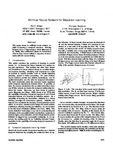
The DeepNet code is written in FORTRAN-95 running under Windows NT 4.0. Preliminary results are very encouraging, both in terms of the exceptional speed of the learning process, and the quality of prediction obtained with test data. For instance, the typical training time using a dataset of several hundred seismic signatures is of the order of seconds on a Dell Workstation 610 configured with 2 Pentium II Xeon processors operating at 400 MHz. It is important to assess the quality of predictions that can be obtained with DeepNet. The network is initially trained using a small subset of the available data: typically, we have used the seismic-to-log correspondence for one, two, or three wells. DeepNet was then used to generate pseudo logs at other wells in the Pompano field. DeepNet Prediction of Well Logs Pompano Test Data: Well_B10 140
120
100
Gamma Ray Response
distance of 200 meters from each well, requiring a resolution accuracy of 5% in terms of the distance from the observation well. Available oilfield information incorporates many datasets with different scales, uncertainties, sample volumes, and relevance. Well logs (e.g., porosity, gamma ray response, and resistivity) provide the most accurate possible sensor-based characterization of the geological formations encountered along the path of a well [24]. On the other hand, low-resolution seismic data are generally used to conduct large-scale field assessments [25]. The specific focus of the research we report in this paper was to develop a methodology that would enable fast and accurate prediction of well pseudo logs from seismic data across an entire oil field. To test the proposed methodology, the Pompano field, located in the Gulf of Mexico, was selected. Pompano is in deep water and has a significant potential for compartmentalized oil. The fine scale heterogeneity caused by the channel depositional environment is well below the resolution of 3D seismic data. The information available to us included 3D seismic data, well logs, core samples, oil location and production profiles. Five seismic variables were provided: the reflected seismic signal, acoustic impedance (AI), and three components of the Hilbert transform of the reflected seismic signal (amplitude, frequency, and phase). Each of the five datasets had 80 megabytes of data with a spatial resolution of 4 km in x and 7 km in y. An x-t plot of the reflected seismic signal is displayed in Fig. 1. For the case of normal incidence, the amplitude of the reflected signal depends on the change in acoustic impedance at the interface between two materials, where AI is the product of density and the speed of sound in the material. The log data is sampled at regular intervals along the well. In Pompano, most wells are not vertical (of the 17 wells studied here, only three are vertical). The DeepLook consortium of petroleum companies provided us with the rate of deviation for each well. We calculated the (x,y,z) coordinates for each data sample in the log data from the seismic data, which have coordinates of (x,y,t), where t is the two way travel time. To convert from t to z, we used a smooth estimates
80
60
40
20
0 1
51
101
151
201
251
301
351
401
451
501
551
601
651
Sequential z Samples NN_predicted log
Actual well log
Fig. 2: DeepNet predicts accurately the gamma ray log using test data from Pompano well B-10
701
For comparison purposes the same pseudo logs were generated using a competing, recently published state-of-the-art neural network algorithm (i.e., the Nadaraya-Watson paradigm [26]). The much more accurate DeepNet results are illustrated in Figure 2. The N-W results are given in Figure 3. For both cases, Pompano well B-10 was used for the prediction test.
References 1. 2. 3. 4. 5. 6.
Prediction of DeepLook Well Logs using Rao's Nadaraya-Watson Net
7.
140
8.
120
Gamma Ray Response
100
9. 80
10. 60
11.
40
20
12.
0 1
51
101
151
201
251
301
351
401
451
501
551
601
651
701
Sequential z Samples NN_predicted log
Actual well log
Fig. 3: Prediction of gamma ray log using a NadarayaWatson algorithm for test well B-10 is less accurate.
13. 14. 15.
Conclusions The DeepNet algorithm represents a new, ultrafast (single iteration) approach to neural network learning for feedforward nets. As such, it has considerable advantages in efficiency (speed, computation cost) over backpropagation. Further more, initial results indicate that it is also has higher prediction accuracy. It is interesting to note that network retraining, typically associated with an excessive cost when using conventional learning, will now become trivial. When combined with the NOGA uncertainty reduction algorithms, our methodology will enable the oil exploration and production industry to gain an unprecedented insight into fluid types and distributions in reservoirs of interest. Acknowledgements This research was performed at the Center for Engineering Science Advanced Research, Computer Science and Mathematics Division, Oak Ridge National Laboratory. Funding was provided by the DeepLook Consortium under Agreement Number ERD-97-1506, and by the Engineering Research Program of the DOE Office of Science under contract DE-AC05-00OR22725 with UT - Battelle, LLC.
16. 17. 18. 19. 20. 21.
22. 23. 24. 25.
26.
M. Hassoun, Fundamentals of Artificial Neural Networks, MIT Press (1995). M. Bishop, Neural Networks for Pattern Recognition, Oxford University Press (1997). M. Beckerman, Adaptive Cooperative Systems, Wiley Interscience (1997). D. White and D. Sofge, Handbook of Intelligent Control: Neural, Fuzzy and Adaptive Approaches, Van Nostrand Reinhold (1992). A. Cichocki and R. Unbehauen, Neural Networks for Optimization and Signal Processing, Wiley (1993). P. Mars, J. Chen, and R. Nambiar, Learning Algorithms, CRC Press (1996). N. Toomarian and J. Barhen, “Learning a Trajectory using Adjoint Functions and Teacher Forcing”, Neural Networks, 5, 473-484 (1992). N. Toomarian and J. Barhen, “Fast Temporal Neural Learning Using Teacher Forcing”, U.S. Patent No. 5,428,710 (March 28, 1995). Y. Chauvin and D. Rumelhart, Backpropagation: Theory, Architectures, and Applications, Lawrence Erlbaum (1995). J. Barhen, S. Gulati, and M. Zak, “Neural Learning of Constrained Nonlinear Transformations”, IEEE Computer, 22(6), 67-76 (1989). J. Barhen, N. Toomarian, and S. Gulati, “Applications of Adjoint Operators to Neural Networks", Appl. Math. Lett., 3(3), 13-18 (1990). N. Toomarian and J. Barhen, “Neural Network Training by Integration of Adjoint Systems of Equations Forward in Time”, U.S. Patent No. 5,930,781 (July 27, 1999). J. Barhen, V. Protopopescu, and D. Reister, “TRUST: A Deterministic Algorithm for Global Optimization”, Science, 276, 1094-1097 (1997). A. Shepherd, Second-Order Methods for Neural Networks, Springer (1997). F. Biegler-König and F. Bärman, “A Learning Algorithm for Multilayered Neural Networks based on Linear Least Squares Problems”, Neural Networks, 6, 127-131 (1993). J. Barhen, R. Cogswell, and V. Protopopescu, “Single Iteration Training Algorithm for Multi-layer Feed-forward Neural Networks,” Neural Proc. Lett, 11(2) (in press, 2000). J. Barhen, D.Reister, and V. Protopopescu, “DeepNet: An Ultrafast Neural Learning Code for Seismic Imaging”, Procs. IJCNN’99, CD-ROM, IEEE Press (1999). R. Myers, Response Surface Methodology, Edwards Bros. (1976). B. Kosko, Fuzzy Engineering, Prentice Hall (1996). A. Dubrawski, “Stochastic Validation for Automated Tuning of Neural Network’s Hyper Parameters”, Robotics and Autonomous Systems, 21, 83-93 (1997). F. Aminzadeh, J. Barhen, C. Glover, and N. Toomarian, “Estimation of Reservoir Parameters using a Hybrid Neural Network”, Jour. of Petroleum Science & Engineering, 24, 49-56 (1999). J. Barhen, D. Cacuci, J. Wagschal, and M. Bjerke, “Uncertainty Analysis of Time-Dependent Nonlinear Systems”, Nuclear Science & Engineering, 81(1), 23-44 (1982). J. Tolma and P. Barton, “On Computational Differentiation”, Comp. Chem. Engin., 22(4/5), 475-490 (1998). P.M. Wong et al, “An Improved Technique in Porosity Prediction: A Neural Network Approach”, IEEE Trans. Geosc. Rem. Sens. , 33(4), 971-980 (1995). J.Schuelke, J. Quirein, and J. Pita, “Prediction of Reservoir Architecture and Porosity Distribution using Multiple Seismic Attributes”, Procs., 30 th Offshore Technology Conf., pp. 83-88 (1998). N.S.V. Rao, et al., "Learning Algorithms for Feedforward Networks Based on Finite Samples," IEEE Trans. on Neural Networks, 7(4), 926-960 (1996).