Psychology Science Quarterly, Volume 50, 2008 (3), pp. 328-344
Understanding and quantifying cognitive complexity level in mathematical problem solving items SUSAN E. EMBRETSON1 & ROBERT C. DANIEL Abstract The linear logistic test model (LLTM; Fischer, 1973) has been applied to a wide variety of new tests. When the LLTM application involves item complexity variables that are both theoretically interesting and empirically supported, several advantages can result. These advantages include elaborating construct validity at the item level, defining variables for test design, predicting parameters of new items, item banking by sources of complexity and providing a basis for item design and item generation. However, despite the many advantages of applying LLTM to test items, it has been applied less often to understand the sources of complexity for large-scale operational test items. Instead, previously calibrated item parameters are modeled using regression techniques because raw item response data often cannot be made available. In the current study, both LLTM and regression modeling are applied to mathematical problem solving items from a widely used test. The findings from the two methods are compared and contrasted for their implications for continued development of ability and achievement tests based on mathematical problem solving items. Key words: Mathematical reasoning, LLTM, item design, mathematical problem solving
1
Dr. Susan Embretson, School of Psychology, Georgia Institute of Technology, 654 Cherry Street, Atlanta, GA 30332-0170, USA; email:
[email protected]
Understanding and quantifying cognitive complexity level in mathematical problem solving items
329
Since its introduction in 1973, the linear logistic test model (LLTM; Fischer, 1973) has been applied widely to understand sources of item complexity in research on new measures (e.g., Embretson, 1999; Gorin, 2005; Hornke & Habon, 1986; Janssen, Schepers, & Peres, 2004; Spada & McGaw, 1985). These applications require not only estimation of LLTM parameters on item response data, but a system of variables that represent theoretically interesting sources of item complexity. Advantages of item complexity modeling with LLTM include elaborating construct validity at the item level, defining variables for item design, predicting parameters of new items, item banking by sources of complexity and providing a basis for item design and item generation. These advantages will be reviewed more completely below. However, despite the many advantages of applying LLTM to test items, it has been applied less often to understand the sources of complexity for operational test items. Instead, item difficulty statistics, such as classical test theory p-values or item response theory bvalues, are modeled from item complexity factors using regression techniques. Often this approach is used because raw item response data cannot be made available. For example, Newstead et al (2006) modeled item difficulty of complex logical reasoning items from the Graduate Record Examination (GRE). Similarly, Gorin and Embretson (2006) modeled item parameters for verbal comprehension items from the GRE while Embretson and Gorin (2001) modeled item parameters for the Assembling Objects Test from the Armed Services Vocational Aptitude Battery (ASVAB). To date, item difficulty modeling has provided validity evidence for many tests, including English language assessments, such as TOEFL (Freedle & Kostin, 1996, 1993; Sheehan & Ginther, 2001) and the GRE (Enright, Morley, & Sheehan, 1999; Gorin & Embretson, 2006). Unfortunately, the studies of item difficulty based on regression modeling have less clear interpretations about the relative impact of the complexity variables in the model. That is, the standard errors often are large since the regression modeling is applied to item statistics rather than raw item response data. Furthermore, the parameters estimated for the impact of the complexity variables are not useful for item banking because the usual properties of consistency and unbiasedness do not extend to the modeling of item statistics. In this paper, applications of LLTM to items from a widely used test of mathematical reasoning will be contrasted with regression modeling of item statistics. The item complexity variables are based on a cognitive theory of mathematical problem solving that was developed for complex items. Prior to presenting the studies on mathematical reasoning, the LLTM and its advantages will be elaborated.
LLTM and related models Several IRT models have been developed to link the substantive features of items to item difficulty and other item parameters. Unidimensional IRT models with this feature includes the Linear Logistic Test Model (LLTM; Fischer, 1973), the 2PL-Constrainted Model (Embretson, 1999) and the Random Effects Linear Logistic Test Model (LLTM-R; (Janssen, Schepers, & Peres, 2004). Also, the hierarchical IRT model (Glas & van der Linden, 2003) could be considered as belonging to this class, if item categories are considered to define substantive combinations of features. In this section, these models will be reviewed.
330
S. E. Embretson & R. C. Daniel
The LLTM (Fischer, 1973) belongs to the Rasch family of IRT models, but item difficulty is replaced with a model of item difficulty. In LLTM, items are scored on stimulus features, qik, which is the score of item i on stimulus feature k in the cognitive complexity model of items. Estimates from LLTM include ηk, the weight of stimulus feature k in item difficulty and θj, the ability of person j. The probability that the person j passes item i, P(Xij=1) is given as follows:
exp(θ j − ∑ k =1 qik ηk ) K
P ( X ij = 1| θ j , q, η) =
(1)
1 + exp(θ j − ∑ k =1 qik ηk ) K
where qi1 is unity and 01 is an intercept. No parameter for item difficulty appears in the LLTM; instead, item difficulty is predicted from a weighted combination of stimulus features that represent the cognitive complexity of the item. That is, the weighted sum of the complexity factors replaces item difficulty in the model. In Janssen et al’s (2004) model, LLTM-R, a random error term is added to the item composite to estimate variance in item difficulty that is not accounted for by the complexity model. The 2PL-Constrained model (Embretson, 1999) includes cognitive complexity models for both item difficulty and item discrimination. In this model, qik and qim are scores of stimulus factors, for item difficulty and item discrimination, respectively, in item i. The model parameter 0k is the weight of stimulus factor k in the difficulty of item i, Jm is the weight of stimulus factor m in the discrimination of item i and θi is defined as in Equation 1. The 2PL-Constrained model gives the probability that person j passes item i as follows: exp(∑ m=1 qimτ m (θ j − ∑ k =1 qik ηk )) M
P ( X ij = 1| θ j , q, η,τ ) =
K
1 + exp(∑ m =1 q imτ m (θ j − ∑ k =1 qik ηk )) M
K
(2)
where qi1 is unity for all items and so J1 and 01 are intercepts. The 2PL-Constrained is the cognitive model version of the 2PL model, since both the item difficulty parameter bi and the item discrimination parameter ai are replaced with cognitive models. Finally, the hierarchical IRT model (Glas & van der Linden, 2003) is similar to the 3PL model, except that the parameters represent a common value for a family of items. The probability is given for person j passing item i from family p, and the item parameters are given for the item family, as follows:
(
P ( X ij p = 1| θ j , ai p , bi p , ci p ) = ci p + 1 − ci p
a (θ − b )) ) 1 +exp( exp( a (θ − b )) ip
j
ip
ip
j
(3)
ip
where aip is item slope or discrimination of item family p, bip is the item difficulty of item family p, cip is lower asymptote of item family p and θj is ability for person j. Thus, in this model, items within family p are assumed to have the same underlying sources of item difficulty, but differing surface features. For example, in mathematical word problems, the same essential problem can be presented with different numbers, actors, objects and so forth. Of
Understanding and quantifying cognitive complexity level in mathematical problem solving items
331
course, substituting surface features can create variability within a family and hence the hierarchical model includes assumptions about the distribution of the item parameters. It should be noted that the original LLTM also can be formulated to represent item families in modeling item difficulty. That is, the qik represent a set of dummy variables that are scored for items in the same family. The random effects version, LLTM-R, can be formulated with dummy variables and, in this case, would estimate variance due to items within families.
Advantages of LLTM and related models If LLTM is estimated with item complexity factors that represent theoretically interesting and empirically supported variables, then applying the model to operational tests has several advantages. First, construct validity is explicated at the item level. The relative weights of the underlying sources of cognitive complexity represent what the item measures. Messick (1995) describes this type of item decomposition as supporting the substantive aspect of construct validity. Second, test design for ability tests can be based on cognitive complexity features that have been supported as predicting item psychometric properties. That is, the test blueprint can be based on stimulus features of items that have empirical support. Third, the empirical tryout of items can be more efficiently targeted. Typically, item banks have shortages of certain levels of difficulty. By predicting item properties such as item difficulty, empirical tryout can be restricted to only those items that correspond to the target levels of difficulty. Furthermore, items with construct-irrelevant features can be excluded from tryout if they are represented by variables in the model. Fourth, predictable psychometric properties can reduce the requisite sample size for those items that are included in an empirical tryout (Mislevy, Sheehan & Wingersky, 1993). The predictions set prior distributions for the item parameters, which consequently reduces the need for sample information. Under some circumstances, predicted item parameters function nearly as well as actually calibrated parameters (Bejar et al, 2003). Fifth, a plausible cognitive model provides a basis for producing items algorithmically. Items with different sources of cognitive complexity can be generated by varying item features systematically, based on the cognitive model. Ideally, these features are then embedded in a computer program to generate large numbers of items with predictable psychometric properties (e.g., Embretson, 1999; Hornke & Habon, 1986 ; Adrensay, Sommer, Gittler & Hergovich, 2006). Sixth, a successful series of studies to support the model of item complexity can provide the basis for adaptive item generation. This advantage takes computerized adaptive testing to a new level. That is, rather than selecting the optimally informative item for an examinee, instead the item is generated anew based on its predicted psychometric properties, as demonstrated by Bejar et al (2003). Finally, score interpretations can be linked to expectations about an examinee’s performance on specific types of items (see Embretson & Reise, 2000, p. 27). Since item psychometric properties and ability are measured on a common scale, expectations that the examinee solves items with particular psychometric properties can be given. However, item estimates based on LLTM and related models go beyond the basic common scale, because the item solving probabilities are related to various sources of cognitive complexity in the items. Stout (2007) views this linkage as extending continuous IRT models to cognitive diagnosis, in the case of certain IRT models.
332
S. E. Embretson & R. C. Daniel
The cognitive complexity of mathematical problem solving items Cognitive complexity level and depth of knowledge have become important aspects of standards-based assessment of mathematical achievement. Cognitive complexity level is used to stratify items in blueprints for many state year-end tests and in national tests. However, obtaining reliable and valid categorizations of items on cognitive complexity has proven challenging. For example, although items with greater cognitive complexity should be empirically more difficult, it is not clear that evidence supports this validity claim. Further, rater reliability even on national tests such as NAEP is not reported. Yet another challenge is some systems for defining cognitive complexity (e.g., Webb, 1999) seemingly relegate the predominant item type on achievement tests (i.e., multiple choice items) to only the lowest categories of complexity. In this study, a system for understanding cognitive complexity of mathematical problem solving items is examined for plausibility. The system is based on a postulated cognitive model of mathematical problem solving which is examined for empirical plausibility using item difficulty modeling. Two approaches to understanding cognitive complexity in items, LLTM and regression modeling, are presented and compared. For both approaches, the development of quantitative indices of item stimulus features that impact processing difficulty is required. Processing difficulty, in turn, impacts psychometric properties. If the model is empirically plausible, support for the substantive aspect of validity (Messick, 1995) or for construct representation validity (Embretson, 1998) is obtained.
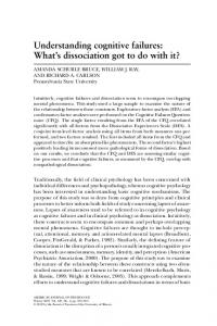
Theoretical background The factors that underlie the difficulty of mathematics test items have been studied by several researchers, but usually the emphasis is to isolate the effects of a few important variables (e.g., Singley & Bennett, 2002; Arendasy & Sommer, 2005; Birenbaum, Tatsuoka, & Gurtvirtz, 1992). The goal in the current study was to examine the plausibility of a model that could explain performance in a broad bank of complex mathematical problem solving items. Mayer, Larkin and Kadane’s (1984) theory of mathematical problem solving is sufficiently broad to be applicable to a wide array of mathematical problems. Mayer et al (1984) postulated two global stages of processing with two substages each: Problem Representation, which includes Problem Translation and Problem Integration as substages, and Problem Execution, which includes Solution Planning and Solution Execution as substages. In the Problem Representation stage, an examinee converts the problem into equations and then in the Problem Execution stage, the equations are solved. Embretson (2006) extended the model to the multiple choice item format by adding a decision stage to reflect processing differences in the role of distractors (e.g., Embretson and Wetzel, 1987). Figure 1, an adaptation of an earlier model (Embretson, 2006), presents a flow diagram that represents the postulated order of processes in general accordance with Mayer et al’s (1984) theory. A major distinction in the model is equation source. If the required equations are given directly in the item, then Problem Execution is the primary source of item difficulty. If the requisite equations are not given directly in the item, then processes are needed to translate, recall or generate equations. Once the equations are available in working mem-
Understanding and quantifying cognitive complexity level in mathematical problem solving items
ENCODE
Encode
INTEGRATION
Find Relations No
333
Word? No Equation Given? Yes
Phase Translation
Knowledge? Yes Retrieve LTM
No
Generate Equation
Transfer STM No
Equation Mapping Complete Set? Yes
Figure 1: Cognitive Model for Mathematical Problem Solving Items
ory, the Problem Execution stage can be implemented. Problem Execution involves 1) planning, in which a strategy for isolating the unknowns is developed and implemented, 2) solution execution, in which computations are made to obtain the unknowns, and 3) decision, in which the obtained solution is compared to the response alternatives. Some items do not require solution planning, however, since the equations are given in a format so that only computation algorithms need to be applied. Several variables were developed in a previous study (Embretson, 2006) to represent the difficulty of the postulated stages in mathematical problem solving. For the Problem Translation stage, a single variable, encoding, was scored as the sum of the number of words, term and operators in the stem. For the Problem Integration stage, several variables were scored to represent processing difficulty for items in which the equation was not given: 1) translating equations from words, 2) number of knowledge principles or equations to be recalled, 3) maximum grade level of knowledge principles to be recalled and 4) generating unique equations or representations for the problem. For some items a special problem representation may be needed; that is, visualization may be required when a diagram is not provided. For the Solution Planning stage, two variables, the number of subgoals required to obtain the final solution and the relative definition of unknowns determine item difficulty. For the Solution Execution stage, the number of computations and the procedural level impact item difficulty. Finally, for the Decision stage, item difficulty is impacted when finding the correct answer involves extensive processing of each distractor. This occurs when the answer obtainable from the stem alone cannot be matched directly to a response alternative.
334
S. E. Embretson & R. C. Daniel
Method Test and item bank. A large set of disclosed items were available from the Quantitative section of the GRE. The Quantitative section contains three types of items; Problem Solving, Quantitative Comparison and Data Interpretation. A Problem Solving item consists of a stem that defines the problem and five unique response choices. The stems range in length and type; some stems are highly elaborated word problems while others contain equations or expressions. A Quantitative Comparison item consists of a short stem and two columns, A and B, that contain either numbers or equations. Each item has the same four response alternatives; “The quantity in A is greater”, “The quantity in B is greater”, “The quantities are equal”, and “The relationship cannot be determined”. Finally, Data Interpretation items consist of a graph, table or chart, a short stem that poses a question about the display and five unique response alternatives. For each item, the GRE item bank parameters were available. In the current study, only the Problem Solving items were modeled because they are used widely on many high stakes tests to measure achievement or ability. Design. Eight test forms had been administered in a previous study to collect item response time data for developing the cognitive model for the mathematical problem solving items (Embretson, 2006). However, item response data were also available and had not been previously analyzed. Each test form contained 43 items, of which 12 items were linking items and the remaining items were a mixture of Problem Solving items and Quantitative Comparison items. A total of 112 Problem Solving items were included across the eight forms. Participants. The participants were 534 undergraduates from a large Midwestern University who were enrolled in an introductory psychology course. The participants were earning credits as part of a course requirement. Procedures. Each participant was randomly assigned a test form. All test forms were administered by computer in a small proctored laboratory. The test administration was not speeded as participants were allowed up to one hour to complete the test form. Nearly all participants completed the test in the allotted time. Cognitive complexity scores. The items were scored for cognitive complexity by multiple raters. All items were outlined for structure prior to scoring. The variables were scored as follows: 1) Encoding, a simple count of the number of words, terms and operators in the item stem, 2) Equation Needed, a binary variable scored “1” if the required equation was not included in the item stem, 3) Translate Equations, a binary variable scored “1” if the equation was given in words in the item stem, 4) Generate Equations, a binary variable scored “1” if the examinee had to generate a unique representation of the problem conditions, 5) Visualization, a binary variable scored “1” if the problem conditions could be represented in a diagram that was not included, 6) Maximum Knowledge, the grade level of the knowledge required to solve the problem (scored from National Standards), 7) Equation Recall Count, the number of equations that had to be recalled from memory to solve the problem, 8) Subgoals Count, the number of subgoals that had to be solved prior to solving the whole problem, 9) Relative Definition, a binary variable scored “1” if the unknowns were defined relative to each other, 10) Procedural Level, the grade level of the required computational procedures to solve the problem, 11) Computational Count, the number of computations required to solve the problem and 12) Decision Processing, scored “1” if extended processing of the distractors was required to reject all but the correct answer.
Understanding and quantifying cognitive complexity level in mathematical problem solving items
335
Results Descriptive statistics. The Rasch model parameters were calibrated using the twelve common items to link item difficulties (bi) across forms using BILOG-MG. Estimates were scaled by fixing item parameters (Mn = 0, Slope = 1), according to typical Rasch model procedures. An inspection of the goodness of fit statistics for items, based comparing expected versus observed response frequencies, indicated that only two of the 112 items failed to fit the Rasch model (p’s < .01). Lowering the criterion for misfit resulted in only one more additional item that failed to fit (p