Understanding Machine Learning Performance with ...

Understanding Machine Learning Performance with Experiment Databases

Joaquin Vanschoren

Jury:

Dissertation presented in partial

Prof. Dr. ir. D. Berlamont, president

fulfillment of the requirements for

Prof. Dr. ir. H. Blockeel, promotor Prof. Dr. M. Bruynooghe

the degree of Doctor in Engineering

Prof. Dr. ir. J. Suykens Prof. Dr. P. Brazdil (University of Porto, Portugal) Prof. Dr. G. Holmes (Waikato University, New Zealand) Prof. Dr. J. Kok (Universiteit Leiden, The Netherlands) UDC 681.3∗I26 May 2010

c Katholieke Universiteit Leuven – Faculty of Engineering ⃝ Address, B-3001 Leuven (Belgium) Alle rechten voorbehouden. Niets uit deze uitgave mag worden vermenigvuldigd en/of openbaar gemaakt worden door middel van druk, fotocopie, microfilm, elektronisch of op welke andere wijze ook zonder voorafgaande schriftelijke toestemming van de uitgever. All rights reserved. No part of the publication may be reproduced in any form by print, photoprint, microfilm or any other means without written permission from the publisher. D/2010/7515/46 ISBN 978-94-6018-206-8

Beknopte samenvatting Het onderzoek in automatische leermethoden en data mining kan aanzienlijk versneld worden wanneer we experimentele onderzoeksresultaten kunnen uploaden naar het internet en verzamelen in applicaties die de data filteren en organiseren. De massale stroom aan experimenten die uitgevoerd worden om nieuwe algoritmes te vergelijken, onderzoekshypothesen te testen en data te modelleren is wellicht erg bruikbaar in verder onderzoek, maar wordt momenteel weggegooid of vergeten. In deze thesis ontwikkelen we een infrastructuur om automatisch experimenten te exporteren naar experiment databanken, databanken die specifiek ontworpen zijn om de details van grote hoeveelheden experimenten, uitgevoerd door verschillende onderzoekers, te verzamelen en om databank queries op te stellen over nagenoeg elk aspect van het leergedrag van leeralgoritmes. Ze kunnen opgezet worden voor persoonlijk gebruik, om resultaten te delen binnen een onderzoekslabo, of om publieke, globale databanken op te zetten. Gelijkaardige trends bestaan in vele andere onderzoeksgebieden, en wij volgen een gelijkaardige strategie door eerst een formeel domeinmodel, een ontologie, op te stellen. Daarna gebruiken we deze ontologie om een XML-gebaseerde taal af te leiden voor het uitwisselen van experimenten, alsook om databankmodellen af te leiden om alle gedeelde resultaten te organiseren. Ten slotte tonen we aan hoe zulke databanken gebruikt kunnen worden om te meta-leren: om nieuwe inzichten te bekomen in het leergedrag van leeralgoritmes. Door vaak niet meer dan een enkele databank query te gebruiken hebben we vaak verrassende nieuwe resultaten bekomen. Zo hebben we gedetailleerde rangschikkingen van experimenten opgesteld, hebben we inzicht gekregen in het gedrag van ensemble-methoden, hebben we verbeteringen voorgesteld voor bepaalde algoritmes, hebben we leercurve-analyses uitgevoerd en hebben we inzicht gekregen in het bias-variance gedrag van leeralgoritmes. We hebben ook meta-modellen gebouwd om geschikte leeralgoritmes en parameterinstellingen te voorspellen en te verklaren. Dit illustreert dat er veel geleerd kan worden door voorgaande leerexperimenten te verzamelen en te hergebruiken, en dat het bouwen van experiment databanken om deze experimenten te bevragen een zeer doeltreffende techniek is om deze data te exploiteren. Vaak bekomen we hierdoor verassende nieuwe inzichten, of interessante nieuwe onderzoeksvragen.

Abstract Research in machine learning and data mining can be speeded up tremendously by moving empirical research results out of people’s heads and labs, onto the network and into tools that help us structure and filter the information. The massive streams of experiments that are being executed to benchmark new algorithms, test hypotheses or model new datasets have many more uses beyond their original intent, but are often discarded or their details are lost over time. In this thesis, we developed a framework to automatically export experiments to experiment databases, databases specifically designed to collect all the details on large numbers of past experiments, performed by many different researchers, and to compose queries about almost any aspect of the behavior of learning algorithms. They can be set up for personal use, to share results within a lab, or to build community-wide repositories. Following similar developments in several other sciences, we first define a formal domain model, an ontology, for experimentation in machine learning, after which we use this ontology to define an XML-based language to exchange experiments, as well as a database model to organize all submitted results. Finally, we demonstrate how such databases can be queried to meta-learn: to gain new insight into learning algorithm behavior. Using often no more than a single database query, we obtained surprising new results. This includes detailed rankings of learning algorithms, insight into the behavior of ensemble methods, suggestions for improvement of certain algorithms, learning curve analyses and insight into the bias-variance behavior of algorithms. We also built meta-models for predicting and explaining the suitability of learning algorithms and parameter settings. This illustrates that much can be learned by collecting and reusing past machine learning experiments, and that building experiment databases to query for them provides an effective way of tapping into this information, often yielding surprising new insight or generating interesting new research questions.

Acknowledgements Although I didn’t realize it at the time, this story started off on a chilly evening in March, as I hurried into an artist’s bar in Leuven one evening to meet the A.I. Reading Club for the first time. I was writing my Master’s thesis at the time, and my daily supervisor, Robby Goetschalckx, convinced me to check it out. It was there that I met the first batch of whimsy and bright colleagues that travelled with me along the road, all of which, I presume, are still trying to get through the reading club’s first book: G¨ odel, Escher, Bach. It was also there that I first met my supervisor, Hendrik Blockeel, in person. Skipping ahead six months, around the same late hour, I was working in my office across the hall from Hendrik, when he came in holding my PhD proposal, saying he had the perfect solution for all my (scientific) problems: experiment databases. Thanks, Hendrik, for giving me a great idea and letting me run with it - even though many thought the idea to be overly ambitious, we showed them :). He has been a great source of inspiration, motivation and insight during these years, teaching me to challenge what is known, to pry open black boxes, and to keep an eye on the bigger picture. He always allowed me to drag him out of his office to show him a surprising new result, and travelled with me by plane, car, rickshaw, junk and rowing boat to far-away conferences. Finally, his eternal good humor and patience helped me soothe over the rough patches of a PhD, making it almost seem easy :). I also wish to thank Luc De Raedt for encouraging me to spread the word, and Maurice Bruynooghe for his trust and leadership. Along me in the trenches was a small army of colleagues that was always there when I needed them. While I cannot possibly comment on all of them here, they are all valiant heroes in their own respect, and created a bustling, creative atmosphere that proved invaluable for nurturing many of the ideas in this work. Learning me the tricks of the trade whilst creating a happy ambiance, there were my first office-mates: Anneleen Van Assche, Celine Vens, Werner Uwents and Stefan Raeymaekers. Anneleen and Celine (a.k.a. Hendrik’s girls) happily allowed me to distract them with tricky questions about ensemble algorithms, databases or other meta-topics. Later, in the ‘girl’s office’, there was Elisa Fromont who, aside from being contagiously enthusiastic, taught me how to play poker and many other games, and gladly cared for the cat when I was

v

vi abroad. With Parisa Kordjamshidi I had many interesting discussions, quite a few about getting to grips with parenthood, and finally, Wannes Meert and Nima Taghipour helped me through the last grueling months of thesis writing. Every once in a while there was the familiar clatter of collapsing stacks of soda cans from Siegfried Nijssen’s office, which I frequented regularly to fire off questions no one else could answer (or simply to borrow the couch). Albrecht Zimmermann and Bj¨ orn Bringmann inspired me with their almost German efficiency and dazzling presentation skills, and Anton Dries manned the Genius bar whenever I ran into computer trouble. Tias Guns recharged me with youthful enthusiasm whenever mine started to wear off, and Fabrizio Costa made sure my whiteboard was always full of new problems to think about, walking in with a “Hey, man!” and launching new ideas. Finally, Maarten Mari¨en, Joost Vennekens, Leander Schietgat and Eduardo Costa helped me to stay fit through regular running and tennis sessions during the lunch break. I promise to come more often now the thesis is finished! I was also lucky to meet many accomplished, inspiring researchers who were very supportive of my dreams, and invited me to come work with them. First, there is the Waikato gang: Geoffrey Holmes, Bernhard Pfahringer and Eibe Frank. They made my stay in New Zealand so fruitful and enlightening that three months abroad seemed to fly by in a flash. Geoff regularly got my day off to a great start by sending me small emails entitled “Inspiration”, “Thoughs?” or “Further pursuits”, in which he challenged me to answer open questions or to verify surprising studies. He taught me to “boldly go where no machine learning researcher has gone before” and, more importantly, he also taught me how to make a mean cappuccino. Bernhard regularly amazed me by coming up with the most perfect explanations for the weirdest of results. Not a week went by without interesting new findings. Peter Reutemann and Dale Fletcher were great office mates and inspired me with their practical solutions to many problems. Furthermore, making sure I got the best out of my time in New Zealand, Jesse, Robert, Michelle, Edmund and Albert regularly invited me to climb a mountain or to go on short trips. I fondly remember the day we drove 300 kilometers through a breathtaking landscape to go skiing on an active volcano, and stopping on the way back to buy swimsuits and do some impromptu hot pooling. Finally, a very special thank you goes out to Kim, Tim, Rebecca and Isobel, who warmly welcomed me into their family, even though I was only supposed to feed their cat :). I had a great time, guys. If any scientific project inspired me in particular, it was the Robot Scientist project in Aberystwyth. I was very lucky to work with Ross King, Larisa Soldatova and Amanda Clare, whose views on the next generation of scientific discovery had a profound impact on this thesis. Larisa taught me everything I know about ontology design, and was remarkably easy to work with. I also

vii thank Qi, Wayne, Andrew, Ken and Jem for the many interesting discussions I had with them. My last visit, to Ljubljana, was shorter but very efficient thanks to Saˇso Dˇzeroski and Panˇce Panov, and Dragi, Ivica, Daniela and Violeta filled my evenings with laughter. Besides Hendrik, Maurice and Geoff, I am very honored to have three more outstanding researchers serving on my Ph.D. committee: Johan Suykens, Pavel Brazdil and Joost Kok. Their detailed feedback contributed greatly to the quality of the final text. I also thank Prof. Berlamont for chairing my defence. I gratefully acknowledge the financial support received for the work performed during this thesis from the Flemish government in GOA grant 2003/08 Inductive Knowledge Bases and from the Flemish Fund for Scientific Research (F.W.O.-Vlaanderen) grant G.0108.06 Foundations of Inductive Databases for Data Mining. F.W.O.-Vlaanderen also supported me with two travel grants. Although also often taken for granted, I would like to thank the sysadmins at the Computer Science department and the LUDIT High Performance Computing Cluster, without whose support I could not possibly have performed the massive amounts of experiments in this thesis. Incidentally, I also thank my laptop for literally breaking in half on it’s own accord, two weeks before I had to send this text in, greatly adding to the thrill of research. Last but definitely not least, I wish to thank my family and friends. I’d especially like to thank my parents, for misunderstanding all my ideas but nodding and smiling all the same, and for not minding me working on Christmas morning too much. Bedankt voor jullie onvoorwaardelijke steun en nooit aflatende geloof in mij! Next, I’d like to thank just a few of my friends, several of which are currently writing up their thesis as well: Adriaan, Wim, Jan & Lore, Joris & Iris, Wouter & Tine, Liesbeth & Thomas, Eveline & Edwin, Yves & Paula, Lies & Jozef, Nele & Robin, Lukas & Joke, Joris & Marijke, An & Markske, Isabelle & Joeri and Karen & Bart. Thanks for all the great and funny moments! Beyond the power of words, I’d like to thank Veerle, my love. Even when I had to burn the midnight oil, or basically any oil available, she was eternally supportive and when things looked grim, she always brought back the sunshine. She’s the bee’s knees. She also gave me a beautiful son, Kobe, now eight months old. Every morning, Kobe’s enthusiastic smile magically makes me realize the beauty of the world. No matter how tired or weary, hearing him say ‘papwa’ always brings me back to

viii life. He taught me that, in a world with seemingly unsurmountable challenges, everything begins with baby steps. Kobe, I hope you can read this soon - there are some pretty pictures in the back ;). Joaquin Vanschoren Leuven, May 2010

Contents Contents

ix

List of Figures

xi

List of Tables

xvi

1 Introduction 1.1 Machine Learning . . . . . . . . . . . . 1.2 Knowledge Discovery: An illustration 1.3 Meta-learning . . . . . . . . . . . . . . 1.4 Experiment Databases . . . . . . . . . 1.5 Goal of this thesis . . . . . . . . . . . 1.6 Roadmap and Contributions . . . . . .

. . . . . .

. . . . . .

. . . . . .

. . . . . .

. . . . . .

. . . . . .

. . . . . .

. . . . . .

. . . . . .

. . . . . .

. . . . . .

. . . . . .

. . . . . .

. . . . . .

1 1 2 9 13 14 15

. . . . . . . . . .

. . . . . . . . . .

. . . . . . . . . .

. . . . . . . . . .

. . . . . . . . . .

. . . . . . . . . .

. . . . . . . . . .

. . . . . . . . . .

. . . . . . . . . .

. . . . . . . . . .

. . . . . . . . . .

. . . . . . . . . .

. . . . . . . . . .

. . . . . . . . . .

. . . . . . . . . .

21 21 23 30 32 40 44 45 47 47 51

Support . . . . . . . . . . . . . . . . . . . . . . . . . . . . . . . . . . . .

. . . . . .

. . . . . .

. . . . . .

. . . . . .

. . . . . .

. . . . . .

. . . . . .

. . . . . .

. . . . . .

. . . . . .

. . . . . .

. . . . . .

. . . . . .

. . . . . .

55 55 58 60 64 68 75

Prelude 2 Meta-Learning 2.1 Introduction . . . . . . . . . . . . . . 2.2 Flavors of meta-learning . . . . . . . 2.3 An algorithm selection framework . . 2.4 The data meta-feature space F . . . 2.5 The algorithm meta-feature space G 2.6 The problem spaces P and P ′ . . . . 2.7 The algorithm spaces A and A′ . . . 2.8 The performance space Y . . . . . . 2.9 The meta-learner S . . . . . . . . . . 2.10 Summary and conclusions . . . . . . 3 Intelligent Knowledge Discovery 3.1 Introduction . . . . . . . . . 3.2 Expert systems . . . . . . . 3.3 Meta-models . . . . . . . . 3.4 Planning . . . . . . . . . . . 3.5 Case-based reasoning . . . . 3.6 Querying . . . . . . . . . .

ix

x

Contents 3.7 3.8

A new platform for intelligent KD support . . . . . . . . . . . . Conclusions . . . . . . . . . . . . . . . . . . . . . . . . . . . . .

Prelude Conclusions

Part I

77 84 85

Organizing Machine Learning Information

Outline Part I

89

4 Experiment Databases 4.1 Motivation . . . . . . . . . . . . . . . 4.2 Experiment databases . . . . . . . . . 4.3 Experiment Repositories in e-Sciences 4.4 Designing Experiment Databases . . . 4.5 Using Experiment Databases . . . . . 4.6 Conclusion . . . . . . . . . . . . . . .

. . . . . .

. . . . . .

. . . . . .

. . . . . .

. . . . . .

. . . . . .

. . . . . .

. . . . . .

. . . . . .

. . . . . .

. . . . . .

. . . . . .

. . . . . .

. . . . . .

91 92 94 97 102 105 108

5 The 5.1 5.2 5.3 5.4

Expos´ e Ontology Introduction . . . . . . Previous work . . . . . The Expos´e Ontology Conclusions . . . . . .

. . . .

. . . .

. . . .

. . . .

. . . .

. . . .

. . . .

. . . .

. . . .

. . . .

. . . .

. . . .

. . . .

. . . .

109 110 114 115 133

6 The 6.1 6.2 6.3

ExpML Markup Language 135 Minimal Information about an ML Experiment . . . . . . . . . 136 From Ontology to Markup Language . . . . . . . . . . . . . . . 139 Conclusions . . . . . . . . . . . . . . . . . . . . . . . . . . . . . 148

. . . .

. . . .

. . . .

. . . .

. . . .

. . . .

. . . .

. . . .

. . . .

7 Anatomy of an Experiment Database 149 7.1 From Ontology to Database Model . . . . . . . . . . . . . . . . 150 7.2 Populating the Database . . . . . . . . . . . . . . . . . . . . . . 156 7.3 Conclusions . . . . . . . . . . . . . . . . . . . . . . . . . . . . . 157 Conclusions Part I

Part II

159

Learning From the Past

Outline Part II

163

8 Interfaces: Hiding the Complexity 165 8.1 Software Components . . . . . . . . . . . . . . . . . . . . . . . 166 8.2 Interfaces . . . . . . . . . . . . . . . . . . . . . . . . . . . . . . 168 8.3 The graphical query tool . . . . . . . . . . . . . . . . . . . . . . 169

Contents 8.4

xi

Conclusions . . . . . . . . . . . . . . . . . . . . . . . . . . . . .

9 Exploring learning behavior 9.1 Model-level analysis . 9.2 Data-Level analysis . . 9.3 Method-Level Analysis 9.4 Conclusions . . . . . .

. . . .

. . . .

. . . .

. . . .

. . . .

. . . .

. . . .

. . . .

. . . .

. . . .

. . . .

. . . .

. . . .

. . . .

. . . .

. . . .

. . . .

. . . .

. . . .

. . . .

. . . .

. . . .

. . . .

Conclusions Part II

173 175 176 184 190 191 195

Finale 10 Summary and Future Work 199 10.1 Summary . . . . . . . . . . . . . . . . . . . . . . . . . . . . . . 199 10.2 Future Work . . . . . . . . . . . . . . . . . . . . . . . . . . . . 202

Appendix A Simple, Statistical and Information-Theoretic Data A.1 Some notes on notation . . . . . . . . . . . . . A.2 Simple features . . . . . . . . . . . . . . . . . . A.3 Normality-related features . . . . . . . . . . . . A.4 Redundancy-related features . . . . . . . . . . . A.5 Attribute-target associations . . . . . . . . . . A.6 Algorithm-specific properties . . . . . . . . . . A.7 Propositional versus relational features . . . . .

Properties . . . . . . . . . . . . . . . . . . . . . . . . . . . . . . . . . . . . . . . . . . . . . . . . .

. . . . . . .

. . . . . . .

207 207 207 209 209 210 212 213

Bibliography

215

Publication List

235

List of Figures 1.1 1.2 1.3 1.4 1.5 1.6

2.1 2.2 2.3 2.4 2.5 2.6 2.7 2.8 3.1 3.2 3.3 3.4

Three Bongard problems (#91,#48 and #54). Adapted from Foundalis (2006) . . . . . . . . . . . . . . . . . . . . . . . . . . An overview of the steps composing the KDD process. Adapted from Fayyad et al. (1996) . . . . . . . . . . . . . . . . . . . . . A scatterplot showing our observations using only the last two features and the hidden target concept (dashed line). . . . . . . A decision tree. The numbers in the leaves show the number of instances in that leaf. . . . . . . . . . . . . . . . . . . . . . . . The data splits (full line) and decision boundary (dashed line) implied by the decision tree. . . . . . . . . . . . . . . . . . . . . A classification problem with a linear pattern as target concept and 200 training examples, and the predictions of a range of learning algorithms over the entire instance space. Selected from Fawcett (2009). . . . . . . . . . . . . . . . . . . . . . . . . . . .

3 4 6 8 8

8

Depiction of three reasons why an ensemble learner could perform better than an individual base-learner. Adapted from Dietterich (2000). . . . . . . . . . . . . . . . . . . . . . . . . . . . . . . . . 24 Two different types of transfer learning in neural networks. Adapted from Brazdil et al. (2009). . . . . . . . . . . . . . . . . . . . . . 27 A comparison of base-learning and meta-learning. . . . . . . . . 29 Rice’s framework for algorithm selection. Adapted from Smith-Miles (2008a). . . . . . . . . . . . . . . . . . . . . . . . . . . . . . . . 31 Proposed framework for meta-learning in Smith-Miles (2008a) (full lines), and our extensions (dashed lines) of this framework. 32 Different data characterization approaches. Adapted from Brazdil et al. (2009). . . . . . . . . . . . . . . . . . . . . . . . . . . . . 34 Structure of a decision tree. Adapted from Peng et al. (2002). . 35 Bias versus variance error (Geurts et al. 2005). . . . . . . . . . 43 The architecture of Consultant-2. Derived from Craw et al. (1992) The StatLog approach. . . . . . . . . . . . . . . . . . . . . . . . The architecture of DMA. Adapted from Brazdil et al. (2009). An illustration of the output of the DMA. The first ranking favors accurate algorithms, the second ranking favors fast ones. Taken from Giraud-Carrier (2005). . . . . . . . . . . . . . . . .

xiii

59 61 62 62

xiv

List of Figures 3.5 3.6 3.7 3.8 3.9 3.10 3.11 3.12 3.13

NOEMON’s architecture. Based on Kalousis and Hilario (2001b). 64 The architecture of IDEA. Derived from Bernstein et al. (2005). 65 Part of IDEA’s ontology. Taken from Bernstein et al. (2005). . 66 The architecture of GLS. Adapted from Zhong et al. (2002). . . 67 The architecture of CITRUS. Derived from Wirth et al. (1997). 69 MiningMart architecture. Derived from Morik and Scholz (2004). 71 The architecture of HDMA. Adapted from Charest et al. (2008). 73 Part of the HDMA ontology. Adapted from Charest et al. (2008). 74 The architecture of AMLA. Derived from Grabczewski and Jankowski (2007). . . . . . . . . . . . . . . . . . . . . . . . . . . . . . . . . 76 3.14 A proposed platform for intelligent KD support. . . . . . . . . 81 4.1 4.2 4.3 4.4 4.5

A hybridized DNA-microarray. . . . . . . . . . . GeneExplorer . . . . . . . . . . . . . . . . . . . . A query on the ALADIN interactive sky atlas. . The architecture of experiment databases. . . . . Experimental methodologies in machine learning

. . . . .

100 100 101 103 105

5.1 5.2 5.3 5.4 5.5 5.6 5.7 5.8 5.9

Representation of individuals. . . . . . . . . . . . . . . . . . . . Representation of properties. . . . . . . . . . . . . . . . . . . . Representation of classes (containing individuals). . . . . . . . An overview of the top-level concepts in the Expos´e ontology. . Experiments in the Expos´e ontology. . . . . . . . . . . . . . . . Experiment workflows. . . . . . . . . . . . . . . . . . . . . . . . The context of a scientific experiment. . . . . . . . . . . . . . . Learner evaluation measures in the Expos´e ontology. . . . . . . The ROC curves (left) and precision-recall curves (right) of two algorithms. The larger the area under the curve, the better the performance. . . . . . . . . . . . . . . . . . . . . . . . . . . . . Learner evaluation procedures in the Expos´e ontology. . . . . . Datasets in the Expos´e ontology. . . . . . . . . . . . . . . . . . Algorithms and their configurations in the Expos´e ontology. . . Algorithms and functions can act as algorithm components. . . Internal learning mechanisms in the Expos´e ontology. . . . . . Algorithm specification in the Expos´e ontology. . . . . . . . . .

111 111 111 117 118 119 120 121

An algorithm implementation, in Expos´e and ExpML. . . . . . A dataset definition, in Expos´e and ExpML. . . . . . . . . . . . An experimental workflow (data preprocessing) in Expos´e and ExpML . . . . . . . . . . . . . . . . . . . . . . . . . . . . . . . An experimental workflow (setup and results) in ExpML . . . . An experimental workflow (setup and results) in Expos´e . . . . Context of an empirical study. . . . . . . . . . . . . . . . . . .

141 143

5.10 5.11 5.12 5.13 5.14 5.15 6.1 6.2 6.3 6.4 6.5 6.6

. . . . .

. . . . .

. . . . .

. . . . .

. . . . .

. . . . .

. . . . .

123 124 128 130 131 132 133

144 146 147 147

List of Figures

xv

7.1 7.2 7.3 7.4 7.5 7.6

The experiment table in the experiment database. . . . . . . . Learning algorithms in the experiment database. . . . . . . . . Datasets and data processing in the experiment database. . . . Performance estimation techniques in the experiment database. Experiment outputs in the experiment database. . . . . . . . . Experimental context and execution data. . . . . . . . . . . . .

150 151 154 154 155 156

8.1 8.2 8.3 8.4 8.5 8.6 8.7

Software Components . . . . . . . . . . . . . . The ExpDB Web Interface . . . . . . . . . . . . The ExpDB Explorer Tool . . . . . . . . . . . . Collapsed query graph . . . . . . . . . . . . . . Expanding the query graph . . . . . . . . . . . Selecting attributes and composing constraints Visualizations in the query interface . . . . . .

166 167 169 170 171 172 174

9.1 9.2 9.3

A graph representation of our query. . . . . . . . . . . . . . . . 176 Performance of all algorithms on dataset ‘letter’. . . . . . . . . 177 A partial graph representation of the extended query, showing how to select kernels (left) and the base-learners of an ensemble method (right). The rest of the query is the same as in Figure 9.1.177 Performance of all algorithms on dataset ‘letter’, including baselearners and kernels. Some similar (and similarly performing) algorithms were omitted to allow a clear presentation . . . . . . 178 The effect of parameter gamma of the RBF-kernel in SVMs on a number of different datasets, with their number of attributes shown in brackets, and the accompanying query graph. . . . . . 179 Ranking of algorithms over all datasets and over different performance metrics. Parameter settings are not fully optimized. . 181 Ranking of algorithms over all binary datasets and over different performance metrics. Parameter settings are not fully optimized. 181 Average rank, general algorithms (non-optimized). . . . . . . . 184 Average rank, specific algorithm setups (non-optimized). . . . . 184 The effect of data size and the number of trees on random forests. The actual dataset names are omitted since they are too many to print legibly. . . . . . . . . . . . . . . . . . . . . . . . . . . . 185 Performance comparison of all algorithms on the monks-problems2 test dataset. . . . . . . . . . . . . . . . . . . . . . . . . . . . . 186 (a) The effect of the number of attributes on the optimal gammavalue. (b) Learning curves on the Letter-dataset. . . . . . . . . 187 (a) J48’s performance against OneR’s for all datasets, discretized into 3 classes. (b) A meta-decision tree predicting algorithm superiority based on data characteristics. . . . . . . . . . . . . 188 (a) Gain of C4.5 over OneR over time and moving average. (b) Number of classes in UCI datasets over time and moving average.189

9.4 9.5 9.6 9.7 9.8 9.9 9.10 9.11 9.12 9.13 9.14

. . . . . . .

. . . . . . .

. . . . . . .

. . . . . . .

. . . . . . .

. . . . . . .

. . . . . . .

. . . . . . .

. . . . . . .

xvi

List of Figures 9.15 A meta-tree learned on a meta-dataset concerning predictive accuracies of trees learned on the monks-problems-2 test dataset. 190 9.16 The average percentage of bias-related error for each algorithm averaged over all datasets. . . . . . . . . . . . . . . . . . . . . . 191 9.17 The average percentage of bias-related error in algorithms as a function of dataset size. . . . . . . . . . . . . . . . . . . . . . . 192

List of Tables 1.1

A dataset representing the second Bongard problem. . . . . . .

5

2.1

Overview of the literature in our extended meta-learning framework. . . . . . . . . . . . . . . . . . . . . . . . . . . . . . . . . .

52

3.1

Comparison of prior meta-learning architectures . . . . . . . . .

78

xvii

A learning experience is one of those things that say: “You know that thing you just did? Don’t do that.” Douglas Adams

Chapter One

Introduction 1.1 Machine Learning The burgeoning field of Machine Learning tries to answer the following question: How can we build computer systems that automatically improve with experience, and what are the fundamental laws that govern all learning processes? (Mitchell 2006) Probably the most quintessential type of learning is the discovery of patterns in series of observations, called knowledge discovery. It is the cornerstone of empirical science: in the 16th century, the detailed astronomical observations of Tycho Brahe allowed Johannes Kepler to discover the empirical laws of planetary motion, and nowadays, machine learning techniques are being used to automatically discover unusual astronomical phenomena in continuous streams of images generated by earth-bound and space telescopes. Using computer algorithms, any hidden regularities can be automatically detected and employed to generate increasingly accurate predictions as more data (experience) is made available. Indeed, many data-intensive empirical sciences now depend on machine learning techniques to accelerate the discovery of patterns in experimental data, for instance to pinpoint the functions of individual genes in living cells, to discover which molecules are active against diseases, and to build highly accurate profiles of internet search engine users and online shoppers.

1

2

CHAPTER 1. INTRODUCTION

The second part of the question goes beyond building learning systems, and tries to discover regularities in the behavior of learning processes themselves. The aim here is to express how learning systems are affected by specific properties of the data they encounter. This can be done theoretically, leading to an interesting body of work called computational learning theory, or empirically, by discovering patterns in the performance of existing learning systems. The latter is called meta-learning, and is the focus of this text. First, Section 1.2 will introduce some basic concepts, after which Section 1.3 explains the importance of meta-learning, leading up to the goal of this thesis stated in Section 1.4. Finally, an outline of the thesis with an overview of its most important contributions is provided in Section 1.6.

1.2 Knowledge Discovery: An illustration In this section, we use a running example to introduce some key concepts of the knowledge discovery process. It may be skipped by those already well-versed in this area. Figure 1.1 shows 3 different examples of Bongard problems 1 , named after the Russian computer scientist M. M. Bongard. A typical problem consists of 6 figures conforming to a specific, hidden rule (shown on the left), as well as 6 counterexamples, which do not conform to that rule (but sometimes conform to the negation of it). The ordering of the boxes has no meaning, i.e. all the boxes on the left side of each problem can be scrambled at will, and there is also nothing magical about the number 6: some variants exist that have more examples or that have more positive than negative examples. Can you discover the hidden patterns? This is an example of a supervised classification problem, a problem in which each observation (each of the boxes) is labeled with a classification of that observation. In this case there are two classes: positive (conforming to the hidden rule) or negative. The goal is to learn the target concept (the hidden rule) based on the given observations, and to use it to predict the class of future, unlabeled observations, such as this one:

1 For

an in-depth discussion of Bongard problems, and a very fundamental approach to solving them, see Foundalis (2006)

1.2. KNOWLEDGE DISCOVERY: AN ILLUSTRATION

+

3

-

1

2

7

8

3

4

9

10

5

6

11

12

+

-

+

-

Figure 1.1: Three Bongard problems (#91,#48 and #54). Adapted from Foundalis (2006)

4

CHAPTER 1. INTRODUCTION

Figure 1.2: An overview of the steps composing the KDD process. Adapted from Fayyad et al. (1996)

1.2.1 The knowledge discovery process To allow a learning algorithm to learn from the given observations, we first need to convert the images into a representation the algorithm understands and that (hopefully) still contains the information needed to discover the hidden pattern. Since the source data is typically stored in databases, this combination of database techniques and machine learning is called knowledge discovery in databases (KDD), described by Fayyad et al. (1996) as follows: KDD is the nontrivial process of identifying valid, novel, potentially useful, and ultimately understandable patterns in data. As illustrated in Figure 1.2, it is a multi-step process: Data selection First, we need to decide which aspects of the problem should be taken into account. Here, we need the boxed images and the labels. Data preprocessing Next, we need to extract useful features from the raw data. In this case, we need to use image processing techniques, e.g. to detect edges, corners, curvature and entire shapes (such as triangles and circles). Data transformation Next, we need to select which of the many generated features are most useful depending on the goal of the task. Possible approaches here are feature selection techniques which check which features seem to correlate with the target attribute, and dimensionality reduction techniques which employ statistical transformations of the data to yield new, but fewer, features composed by combining several other ones. Data mining The actual learning step in the knowledge discovery process is called data mining, in which we employ a learning algorithm to build a model of the prepared data. As we shall discuss shortly, different algorithms will perform very differently on different data configurations, and selecting and modifying learning algorithms is a very involved process.

1.2. KNOWLEDGE DISCOVERY: AN ILLUSTRATION

5

Table 1.1: A dataset representing the second Bongard problem. # 1 2 3 4 5 6 7 8 9 10 11 12 13

#△ 1 1 2 1 2 2 1 1 2 2 2 2 0

#black△ #△

1 1 0.5 0 0.5 0 0 1 0 1 1 0 0

#△ #shapes

0.33 0.2 0.4 0.17 0.33 0.4 0.33 0.2 0.4 0.33 0.33 0.33 0

... ... ... ... ... ... ... ... ... ... ... ... ... ...

P

y(!) #! i

0.75 0.8 0.5 0.8 0.75 0.7 0.3 0.65 0.4 0.3 0.45 0.25 0.3

P

y(♦) #♦

i

0.25 0.6 0.25 0.4 0.35 0.25 0.8 0.8 0.55 0.6 0.85 0.7 0.4

class + + + + + + ?

Interpretation Finally, the model produced by the learning algorithm needs to be evaluated for correctness and interpreted in order to speak of ‘knowledge’. Typically, the first models will not be satisfactory, and the whole process will typically be reiterated and adjusted repeatedly.

1.2.2 Data preprocessing We now try to learn the target concept behind the second Bongard problem in Figure 1.1. We assume the data preprocessing and transformation steps have been completed, providing us with an attribute-value representation of the given images. This is the simplest form of representing data: a table in which each row is one observation (called an instance) and each column is a measurable property (called an attribute or a feature) of each of the figures. In Table 1.1, we have numbered the boxes as indicated in Figure 1.1 (number 13 is the unlabeled example shown above), and show the values of the following features: • • • • • •

The The The The The The

number of triangles (the same can be done for squares and circles) ratio of black triangles over all triangles ratio of triangles over all shapes average Y-coordinate (between 0 and 1) of all black shapes average Y-coordinate (between 0 and 1) of all white shapes target feature: positive, negative or unknown

6

CHAPTER 1. INTRODUCTION

?

Figure 1.3: A scatterplot showing our observations using only the last two features and the hidden target concept (dashed line). This representation transforms each observation into a single point in a highdimensional space spanned by the identified features. The subspace spanned by the last two descriptive features is shown in Figure 1.3. The target concept may be clear by now: in the positive examples, all black shapes are positioned above the white shapes and vice versa. With these two dimensions, the target concept is quite straightforward. If we generate many more examples beyond the 12 given by Bongard, all positive examples will be above the dashed diagonal line and all negative ones below. In real-world situations, the features will usually not be this predictive, and many more features may have to be combined in order to provide a good model of the data. Also, more often than not, there is noise in the data: the labels or attribute values of some instances might be wrong, meaning that a completely correct solution is impossible, and that we must be careful not to model this noise (a problem known as overfitting). Finally, there may easily be millions of examples, such as credit card transactions or web searches. We can now provide a more formal definition of our learning problem: Supervised classification is the task of learning from a set of classified training examples (x, c(x)), where x ∈ X (the instance space) and c(x) ∈ C (a finite set of classes), a classifier function f : X → C such that f approximates c (the target function) over X.

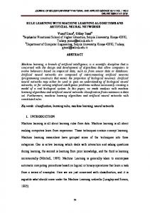
1.2.3 Modeling the data One possible learning algorithm to address this classification problem is a decision tree learner, which assumes that the data can be modeled using a decision tree, as illustrated in Figure 1.4.

1.2. KNOWLEDGE DISCOVERY: AN ILLUSTRATION

7

1.2.3.1 Training A decision tree is trained by recursively choosing a feature and generating a test on that feature that splits the data in multiple parts. The quality of a split is defined by how cleanly it separates the values of the target feature, in this case how well the positive examples are separated from the negative ones. There exist several ways to calculate this, but perhaps the most common is the information-theoretic metric of information gain ratio, which quantifies to which degree the separation of labels is cleaner than before the extra split was added (a formal definition is given in Appendix A). We start off with a single node containing all observations, and after each split, the data points move down to their respective branch, and stored in so-called leaf nodes. The model is then further refined by choosing a leaf node and splitting it further. When we train a decision tree learner2 with our 12 examples, this yields the decision tree shown in Figure 1.4, consisting of two splits: first on the ‘average Y-coordinate of all white shapes’, then on the ‘average Y-coordinate of all black shapes’. These splits are also shown in Figure 1.5: the first split, the vertical line, already yields a good model (only 1 example was misclassified), while the second split further refines it. Also shown is the decision boundary, separating positive from negative examples according to the final model. 1.2.3.2 Interpretation and testing The decision tree’s solution to the Bongard problem is: “The average Y-position of the white shapes is smaller or equal to 0.4, or otherwise the average Yposition of the black shapes is larger than 0.7”. While this is correct according to Bongard’s 12 examples, it is only an approximation of the actual concept, indicated by the diagonal line in Figure 1.3. Indeed, when looking at our test example (the one whose label we want to predict), we see that the decision tree learner classifies it as a positive example, while it is, in fact, a negative one. To be fair, the decision tree learner could have approximated the target concept better if it was given more examples. In Figure 1.6 we show a problem with a similar target concept (a non-axis-parallel straight line) and 200 examples. We see that also in this case, the decision tree approximates the target with a steplike function. Since it can only make axis-parallel splits, it will never be able to match the target concept exactly, and can only approximate it by building a very complex decision tree, resulting in very tiny steps. However, another data transformation step (see Section 1.2.1) could have created a feature equal to the ratio of the final two descriptive features, in which case the decision boundary would have become an axis-parallel line, and a decision tree with a single node would have sufficed to correctly model it. The performance of a learning algorithm thus depends greatly on specific properties of the data at hand, and understanding such relationships is a key aim of this thesis. 2 We

used WEKA’s J48 implementation, with the minimal leaf size set to 1.

8

CHAPTER 1. INTRODUCTION

avg Y white