underwater detection, classification and localisation - Technische ...

UNDERWATER DETECTION, CLASSIFICATION AND LOCALISATION: IMPROVING THE CAPABILITIES OF TOWED SONAR ARRAYS

ii

UNDERWATER DETECTION, CLASSIFICATION AND LOCALISATION: IMPROVING THE CAPABILITIES OF TOWED SONAR ARRAYS

Proefschift ter verkrijging van de graad van doctor aan de Technische Universiteit Delft, op gezag van de Rector Magnificus prof. ir. K.C.A.M. Luyben; voorzitter van het College voor Promoties, in het openbaar te verdedigen op woensdag 20 april 2011 om 10.00 uur door

Mathieu Edouard Guy Didier COLIN Ingénieur Ecole Nationale Supérieure des Etudes et Techniques d’Armement, Brest, Frankrijk geboren te Straatsburg, Frankrijk

Dit proefschrift is goedgekeurd door de promotor: Prof. dr. D.G. Simons Copromotor: Dr. ir. G. Blacquière

Samenstelling promotiecommissie Rector Magnificus,

voorzitter

Prof. dr. D.G. Simons,

Technische Universiteit Delft, promotor

Dr. ir. G. Blacquière,

Technische Universiteit Delft, copromotor

Prof. dr. Y. Pétillot,

Heriot-Watt University

Prof. dr. ir. C.P.A. Wapenaar,

Technische Universiteit Delft

Prof. dr. R. Curran,


Prof. dr. W. A. Mulder,


Dr. X. Lurton,

French Research Institute for Exploitation of the Sea

Published and distributed by: Netherlands Organisation for Applied Scientific Research (TNO) Postbus 96864 2509 JG Den Haag ISBN-13 978-90-5986-378-1 Copyright 2011 by M.E.G.D. Colin All rights reserved. No part of the material protected by this copyright notice may be reproduced or utilized in any forms or by any means, electronic or mechanical, including photocopying, recording or by any information storage and retrieval system, without written permission from the author: M.E.G.D. Colin, TNO, P.O. Box 969864, 2509 JG, The Hague, The Netherlands. Printed in The Netherlands

Elements from the cover art are adapted from The book of Kells, 800, Trinity College, Dublin.

iv

Contents

1 Introduction

1

1.1

The enemy below . . . . . . . . . . . . . . . . . . . . . . . . . . . . .

2

1.2

Peering through the depths

. . . . . . . . . . . . . . . . . . . . . . .

4

1.3

A versatile sensor: the towed hydrophone array . . . . . . . . . . . .

8

1.4

Advanced Signal processing for an advanced sensor . . . . . . . . . .

11

1.4.1

Detection . . . . . . . . . . . . . . . . . . . . . . . . . . . . .

11

1.4.2

Localisation . . . . . . . . . . . . . . . . . . . . . . . . . . . .

12

1.4.3

Classification . . . . . . . . . . . . . . . . . . . . . . . . . . .

12

1.5

Towed array sonar experimental data . . . . . . . . . . . . . . . . . .

14

1.6

Contributions . . . . . . . . . . . . . . . . . . . . . . . . . . . . . . .

16

2 Detection with Passive Synthetic Aperture Sonar 2.1

17

Ideal case . . . . . . . . . . . . . . . . . . . . . . . . . . . . . . . . .

20

2.1.1

Conventional beamformer response . . . . . . . . . . . . . . .

20

2.1.1.1

Response of the ambient noise. . . . . . . . . . . . .

22

2.1.1.2

Response of the interferer. . . . . . . . . . . . . . . .

23

2.1.1.3

Response of the narrowband source. . . . . . . . . .

25

Integrating snapshots . . . . . . . . . . . . . . . . . . . . . . .

26

2.1.2.1

Incoherent integration . . . . . . . . . . . . . . . . .

28

2.1.2.2

Coherent integration : Synthetic aperture . . . . . .

30

Performance analysis . . . . . . . . . . . . . . . . . . . . . . .

35

2.1.3.1

35

2.1.2

2.1.3

Performance criteria . . . . . . . . . . . . . . . . . . v

2.1.3.2

Performance comparison . . . . . . . . . . . . . . . .

38

Summary and discussion . . . . . . . . . . . . . . . . . . . . .

41

Realistic case with perturbations . . . . . . . . . . . . . . . . . . . .

42

2.2.1

Description of the perturbations . . . . . . . . . . . . . . . . .

42

2.2.2

Effect of the perturbations . . . . . . . . . . . . . . . . . . . .

44

2.2.3

Compensation of phase mismatch between snapshots . . . . .

49

2.2.3.1

Description of the phase compensation . . . . . . . .

49

2.2.3.2

Limitations of the phase compensation . . . . . . . .

50

2.2.3.3

Inverse beamforming in combination with ETAM . .

51

Experimental results . . . . . . . . . . . . . . . . . . . . . . .

51

2.2.4.1

2001 Experiment . . . . . . . . . . . . . . . . . . . .

51

2.2.4.2

2003 Experiment . . . . . . . . . . . . . . . . . . . .

54

Summary and Conclusion . . . . . . . . . . . . . . . . . . . . . . . .

54

2.1.4 2.2

2.2.4

2.3

3 Localisation with Passive Sonar using Model-Based Methods

57

3.1

Considerations on passive ranging . . . . . . . . . . . . . . . . . . . .

58

3.2

Recursive estimation . . . . . . . . . . . . . . . . . . . . . . . . . . .

61

3.2.1

Narrowband signals . . . . . . . . . . . . . . . . . . . . . . . .

66

3.2.1.1

Design of a processor . . . . . . . . . . . . . . . . . .

68

3.2.1.2

Simulation

. . . . . . . . . . . . . . . . . . . . . . .

71

3.2.1.3

Measured data . . . . . . . . . . . . . . . . . . . . .

76

3.2.1.4

Summary . . . . . . . . . . . . . . . . . . . . . . . .

79

Broadband signals . . . . . . . . . . . . . . . . . . . . . . . .

80

3.2.2.1

Time delay estimation . . . . . . . . . . . . . . . . .

80

3.2.2.2

Kalman estimator . . . . . . . . . . . . . . . . . . .

85

Batch methods . . . . . . . . . . . . . . . . . . . . . . . . . . . . . .

86

3.3.1

Bearings-Only Target Motion Analysis . . . . . . . . . . . . .

87

3.3.2

Time delay based Target Motion Analysis . . . . . . . . . . .

89

3.3.3

Performance analysis and comparison . . . . . . . . . . . . . .

92

3.3.3.1

Precision . . . . . . . . . . . . . . . . . . . . . . . .

92

3.3.3.2

Observability . . . . . . . . . . . . . . . . . . . . . .

94

Performance comparison . . . . . . . . . . . . . . . . . . . . .

95

3.2.2

3.3

3.3.4 3.4

Summary and conclusion . . . . . . . . . . . . . . . . . . . . . . . . . 100 vi

4 Classification with Active Sonar using BPSK Waveforms 4.1

Doppler sensitive waveforms . . . . . . . . . . . . . . . . . . . . . . . 103 4.1.1

4.2

4.3

A zoo of pulses . . . . . . . . . . . . . . . . . . . . . . . . . . 104 4.1.1.1

Comb spectrum pulses . . . . . . . . . . . . . . . . . 104

4.1.1.2

Smooth spectrum pulses . . . . . . . . . . . . . . . . 105

4.1.2

BPSK pulse . . . . . . . . . . . . . . . . . . . . . . . . . . . . 106

4.1.3

Limitations of the BPSK waveform . . . . . . . . . . . . . . . 107 4.1.3.1

High data volume . . . . . . . . . . . . . . . . . . . . 107

4.1.3.2

Sensitivity to Doppler perturbation . . . . . . . . . . 108

Experimental results . . . . . . . . . . . . . . . . . . . . . . . . . . . 112 4.2.1

Experiment description . . . . . . . . . . . . . . . . . . . . . . 112

4.2.2

Experimental ambiguity function . . . . . . . . . . . . . . . . 113

4.2.3

Signal processing . . . . . . . . . . . . . . . . . . . . . . . . . 114

4.2.4

Effect of topography on classification performance . . . . . . . 114

4.2.5

Classification results . . . . . . . . . . . . . . . . . . . . . . . 115

Summary and Conclusions . . . . . . . . . . . . . . . . . . . . . . . . 118

5 Conclusion and perspective 5.1

5.2

101

119

Conclusion . . . . . . . . . . . . . . . . . . . . . . . . . . . . . . . . . 120 5.1.1

Detection . . . . . . . . . . . . . . . . . . . . . . . . . . . . . 120

5.1.2

Localisation . . . . . . . . . . . . . . . . . . . . . . . . . . . . 120

5.1.3

Classification . . . . . . . . . . . . . . . . . . . . . . . . . . . 121

Perspective . . . . . . . . . . . . . . . . . . . . . . . . . . . . . . . . 122

A Probability of False Alarm

125

B Phase unwrapping algorithm

129

C Cram` er-Rao Lower Bounds

133

C.1 CRLB for broadband bearing estimation . . . . . . . . . . . . . . . . 134 C.2 CRLB for Bearing-Only Target Motion Analysis . . . . . . . . . . . . 136 C.3 CRLB for Time Delay Target Motion Analysis . . . . . . . . . . . . . 137 List of Symbols and Notations

139 vii

List of Acronyms

146

Bibliography

147

Summary

159

Samenvatting

163

Acknowledgments

167

Curriculum Vitae

171

viii

Chapter 1

Introduction

Figure from a patent for a Piezo-Electric Signalling Apparatus filed by Paul Langevin in 1923 [1]

2

CHAPTER 1. INTRODUCTION

”Here there be monsters” The fascination of the undersea world: The Leviathan (Gustave Doré)

Despite being more naturally adapted to walking on land, mankind has always been attracted to travelling on or in water for several purposes: feeding, travelling, harvesting resources, hiding, or, of course, just out of sheer curiosity. In any case, the underwater environment is very mysterious and therefore fascinating to us for various reasons. Most of Earth’s surface is covered by water and holds many riches of different kinds the quantity of which we can only suspect. It is an environment with very varied and dynamic flora, fauna and physics that we are only beginning to grasp. The depths of the sea are remotely accessible and difficult to monitor, which makes them even more intriguing for us, but also the perfect hiding place for someone who wishes to keep a secret agenda.

1.1

The enemy below

The fact that one cannot see very far underwater made it attractive for amateurs of clandestine operations to make use of the underwater concealing properties. The use

1.1. THE ENEMY BELOW

3

Figure 1.1: Cornelis van Drebbel’s oar propelled underwater craft (Lithography by G. W. Tweedale, 1626).

of underwater crafts was imagined very early and first put in application around 1620 in the Thames river by Cornelius van Drebbel (see figure 1.1), a Dutch inventor. Submarine development has progressed ever since, evolving from propulsion with oars, via propellers powered by compressed air, diesel electrics and nuclear power plant to finally air independent propulsion. Modern submarines come in all sizes ranging from the 175 m long Russian Typhoon SSBN (Submersible Ship Ballistic Nuclear, Ballistic Missile Submarine) to the Iranian midget submarine Ghadir, which can accommodate a crew of two, see figure 1.2. Submarines are mostly used for military purposes, such as anti-submarine warfare (ASW) missile delivery, anti-surface warfare, intelligence gathering, mine-laying or special forces delivery but also in criminal or terrorist enterprises. Drug dealers in South America as well as armed groups in Sri-Lanka have been reported to design small submarines for drug and weapons trafficking [2, 3]. The progress of technology and the diffusion of knowledge has made it possible for any small country or wealthy organisation to build its own submarine. All these submarines have always represented a potential threat to national security in one way or another. During World War I, and World War II, German submarines would attack Allied convoys to prevent transport of goods across the Atlantic. During the cold war, the major concern was to be able to track all Soviet SSBNs at all times in the event of a nuclear exchange. Recently the most likely threat is judged to be either

4


25 m 175 m

Figure 1.2: Russian Typhoon class ballistic missile submarine and Iranian “Ghadir” coastal submarine.

small countries operating very silent diesel-electric submarines or a terrorist attack from a midget submarine. The ability to detect and localise a hostile underwater vehicle reduces the potential of destruction it can inflict. More concretely, it is in the interest of any government that wishes to protect its assets, routes of communications and civilian population to have the dissuasive capability to deter such an attack.

1.2

Peering through the depths

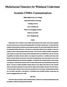
While most of what is happening all over the globe in the atmosphere can be discreetly observed by means of countless satellites sensing the whole electromagnetic spectrum, the physical properties of water in general, and seawater in particular, make it so that most electromagnetic waves are too strongly attenuated after even a few centimetres of propagation underwater to measure anything. For that reason, underwater observation by means of electromagnetic waves is very difficult, in particular from a satellite. There are a few marginal exceptions. Indeed, the electromagnetic absorption spectrum of seawater shown in figure 1.3, allows limited propagation for blue-green light (wavelength in air of 300 nm to 400 nm). This opportunity has been investigated for a few applications. For instance, blue-green lasers are used for the detection of mines in the surf zone1 [4] or for tactical undersea communication [5]. 1

The surf zone is the area of the sea where surface waves break against the coast.

5

1.2. PEERING THROUGH THE DEPTHS

It was considered to use the same lasers to detect submarines [6], but the latter can submerge at depths for which the signal to noise ratio (SNR) of such systems is not sufficient to achieve detection, due to the increased propagation loss. Moreover, the beam of such a laser can only cover a very small area compared to the total surface to be searched. Another remarkable, yet mildly successful, application is the use of bio-luminescence to detect submarines. Some species of phytoplankton liberate photonic energy when shaken [7]. This light can be observed when one waves one’s hand underwater at night or in the wake of a submarine. However this indiscretion is rarely

Optical Absorption [dB/km]

15

10

10

10

5

10

0

10

10

2

10

3

4

5

6

7

10 10 10 10 10 Wavelength in air [nm] (a) Measured EM absorption

8

10

9

Acoustical Absorption [dB/km]

strong enough to allow detection of a submarine from a satellite. 2

10

1

10

0

10

−1

10

−2

10

0

10

1

2

10 10 Frequency [kHz] (b) Empirical sound absorption in seawater, the thick line denotes usual ASW frequencies

Figure 1.3: Measured electromagnetic [8, 9] at optical wavelengths and empirical acoustic absorption [10, 11] of waves in seawater.

While electro-magnetic waves propagate poorly underwater, acoustic waves propagate very well and are much less attenuated, depending on their wavelength (see figure 1.3). One of the first practical scientific applications of acoustic propagation was the measurement of the bulk modulus of water by Colladon and Sturm in 1826 (see pages 125 and 129). A first attempt at acoustic localisation was a navigation acoustic system for lightships at night or in dense fog in the beginning of the 1900s [12]. A pulse would be emitted by an underwater gong at the same time as a foghorn would be blown. Other ships would be fitted with a hydrophone and the operator would estimate the range of the remote transmitter by comparing the time difference between the underwater and airborne sound arrivals, the speed of sound in air being

6


four times slower than in water. As soon as submarines started to represent a real threat in a conflict and as soon the current state of the art allowed it, acoustic waves were used to detect, localise and classify submarines. These same waves are used by submarines to find their prey or evade their hunter. A major breakthrough in the field of underwater acoustics transmission and measurement was the invention of a piezoelectric transducer by Paul Langevin (figure 1.4) assisted by Constantin Chilowsky2 during World War I [13–15].

Figure 1.4: Paul Langevin (1872-1946), one of the inventors of the quartz sandwich transducer.

He used the work of the Curie brothers [16] and Gabriel Lippmann [17] on piezoelectricity as well as his own research results to design a device using the electromechanic conversion due to the piezoelectric effect of quartz crystals. This design 2

The system performance became operationally relevant with the addition of an amplifying device by Beauvais and Brillouin. This amplifier could not have been designed without the contribution of P. Pichon who faced a potential firing squad for desertion to bring triods back to France to support the war effort [13].

7

1.2. PEERING THROUGH THE DEPTHS

Pre-stressed rod Piezoelectric ceramic elements

Pre-stress bolt

Pre-stress bolt

Electrodes Pavilion

Figure 1.5: Schematics of a Tonpilz transducer.

offered a much better efficiency than the electromagnetic technology used in any underwater transducers that far. While natural crystals such as Quartz were used by Langevin in his pioneering experiments, modern transducers are mostly built with baked ceramics (such as lead-zirconium-titanate (PZT) or PolyVinylidine DiFluoride (PVDF)) or grown crystals (such as lead-magnesium-niobate-lead-titanate, PMNPT), which offer better electro-mechanic properties and are easier to shape. A typical arrangement of such ceramics is the Tonpilz transducer, shown in figure 1.5, invented by Langevin [18]. Hollowed ceramics cylinders are arranged on a pre-constraint rod that maintains stress on the ceramics. The electrodes convey the desired electromagnetic wave that is converted into a mechanic wave by the piezoelectric ceramics.

The principles discovered by Langevin and other scientists led to the development of a paraphernalia of submarine detecting devices worldwide. However, it is only after World War II, through the race to arms during the Cold War, that the submarine reached its full terrifying potential of destruction. A number of nations acquired or developed SSBNs that can stay submerged virtually indefinitely. A single of these submarines, if undetected, could bring cataclysmic annihilation to a whole continent at once. It became a crucial concern for navies around the world to track these Leviathans at all time, and preferably from as far as possible. Moreover, the accumulated experience in underwater acoustics of the time clearly pointed to the necessity of taking the complexity of propagation of sound in the ever varying oceanic medium into account. This prompted the further development of an already existing device, the towed hydrophone array.

8


1.3

A versatile sensor: the towed hydrophone array

To allow sensing of the wave propagated from a source at a great distance, in a noisy environment, one must have a sensor that gathers many wavelengths of the propagated wave [19]. In water, acoustic wavelengths that are relevant for the sensing of submarines are of the order of one metre3 . Therefore, ASW sensors, such as passive arrays towed by surface ships or the Sound Surveillance System (SOSUS) [20], can reach dimensions of several kilometres. Mounting such a sensor on the hull of a ship poses limits to the maximum size of the sensor. Some of these sensors, like SOSUS, are deployed at fixed locations, but this is not always operationally convenient. A technological solution that allows deploying an underwater acoustic sensor of long aperture, at virtually any depth so as to make the best of the propagation conditions, while sweeping through an area or pursuing a target, is the towed hydrophone array. A towed hydrophone array is a collection of hydrophones arranged in a line, most often in a hose as it offers the best hydrodynamic behaviour, meant to be towed behind a platform (surface ship or submarine, autonomous or manned). The hose is usually filled with oil so as to have neutral buoyancy, while protecting the electronics from the conducting sea water. Modern towed arrays are also fitted with non acoustic sensors that help ascertain the attitude and position of the array at all times. Another advantage of towing a sensor is that, instead of mounting it on the platform, the sensor is more isolated from the noise radiated by its towing platform. Indeed, depending on the type of arrays, these sensors can be towed at distances of the order of kilometres from the ship. Finally the sonar can be towed at any depth, especially under the surface layer, often present, shown in figure 1.6. Most of the energy transmitted by hull mounted sonars, which were for a long time the main ASW sensor, is refracted directly downwards, to the seafloor or trapped in the surface layer, thus leaving a shadow zone in which submarines often seek acoustic shelter. The first towed hydrophone array, known as “The Eel” was developed in the USA 3

The sound speed in sea water is usually close to 1500 m/s and the frequencies radiated by submarines are usually lower than 1500 Hz resulting in wavelengths of 1 m or longer. Likewise 1500 Hz is a typical frequency used with Low Frequency Active Sonars (LFAS).

1.3. A VERSATILE SENSOR: THE TOWED HYDROPHONE ARRAY

9

0 100 200

Depth [m]

300 400 500 600 700 800 900 1000 1460 1480 1500 0 Sound Speed [m/s]

1

2

3

4

5 Range [nm]

6

7

8

9

Figure 1.6: Typical North Atlantic sound speed profile and corresponding ray trace. The grey area represents the shadow zone in which only a small amount of acoustic energy propagates from a surface source.

as early as World War I [21]. It has known many developments since, adapting itself to the different challenges posed by the tactical requirements of the time. Its use started to become widespread during the Cold War. NATO (North Atlantic Treaty Organization) naval forces employed it to passively detect and track Soviet submarines around the globe. These submarines lacked advanced silencing measures and were usually detected passively, through their acoustic indiscretions, using very long (over 1000 m) towed arrays [21]. However, a few decades of cloak and dagger spying and technological development [22, 23] allowed the USSR to deploy much quieter submarines by the end of the eighties. Around the same time, the collapse of the Warsaw pact shifted the strategic objectives of NATO. The most immediate submarine threat shifted from the less menacing Soviet nuclear submarines to modern diesel electric submarines acquired by rogue nations around the globe. These cheaper submarines have the potential to be quieter than their nuclear counterparts and operate preferably in coastal and shallow waters, closer to their targets. This prompted a change in towed array sonar development, as one could rely less and less on the passive indiscretions of the enemy submarine. Towed arrays became smaller and were used in both passive mode and active mode (in combination with a towed source as shown in figure 1.7), although mostly in the latter. The long passive towed arrays of the Cold War are impractical to deploy in shallow water for several reasons:

10


Towed source Platform

Towed array Target

Figure 1.7: Sketch of an LFAS sonar system (Towed array and source) towed by a frigate (platform), pinging at a submarine (target).

- Shallow waters are plagued by much more noise than deeper waters, partly due to increased human activity around the coasts, making passive detection more challenging. - Long arrays limit the manoeuvrability of the towing platform. - They are dangerous to tow in waters shallower than their length, as they might rake the bottom. Therefore, LFAS systems became the sensors of choice to detect submarines in shallow waters. The optimal frequency band to detect a submarine actively is slightly higher than the frequency band4 used for passive detection, allowing a scaling down of the towed array to a few tens of meters [24]. Passive sonar was still not abandoned for a number of reasons. Some target, such as Go-Fast powerboats used in drug smuggling, have a very low Target Strength [19] and are very difficult to detect actively but do radiate strong noise. Broadcasting with an active sonar does not only betray the position of the platform but can also have an influence on the surrounding marine life, making the use of passive sonar preferable in certain situations, despite the reduced size of the towed array compared to the longer dedicated passive towed arrays. 4

The frequency band used for LFAS is low enough to ensure low absorption losses and chosen at a location of the spectrum where both shipping noise and ocean ambient noise are low.

1.4. ADVANCED SIGNAL PROCESSING FOR AN ADVANCED SENSOR

1.4

11

Advanced Signal processing for an advanced sensor

The topic of this thesis is the development of advanced signal processing algorithms for these shorter towed arrays, both in their active and passive mode of use. The chapters have been structured according to three phases used in ASW: Detection, Localisation and Classification.

1.4.1

Detection

In signal processing, detection is the process of making a decision concerning the occurrence of an event. In the case of passive sonar, this event is the radiation of sound by an acoustic source. The decision of the presence of a source is made when the signal measured exceeds a certain threshold. In the case of passive towed array sonar, data is collected by an array of hydrophones. In the past, an operator would listen directly to the sound collected by the hydrophones and carry out detection himself. The combination of the ear and brain of a trained operator is difficult to outperform through signal processing, but there are processing operations that an operator cannot handle. For instance, the data collected by a modern passive towed array sonar consists of channels of acoustic time series originating from tens of hydrophones that are too many for an operator. Modern sensor signal processing strives to reduce the load of the operator as much as possible, possibly even replacing him or her. The data collected by these hydrophones contains signal from sources of interest, interfering sources (such as the towing platform or merchant traffic) and ambient noise [19]. The purpose of this linear arrangement of hydrophones is to directionally isolate the signal of interest from the ambient noise and the interfering sources. The hydrophones need to sample the acoustic field with a spacing small enough to respect the Nyquist criterion of spatial sampling

5

and long enough to

collect uncorrelated noise realisation, and offer a spatial aperture, at frequencies of interest for passive sonar. The total length of the array determines the capacity to spatially discriminate a given signal from another source and ambient sound [25]. This 5

In order to avoid aliasing, the maximum spacing between sensors of an array sampling should be no longer than half of the smallest wavelength measured by the sensor.

12


is performed through a class of signal processing algorithms known as beamformers. In Chapter 2, we concentrate on the problem of beamforming while considering one method in particular. This method, known as Passive Synthetic Aperture Sonar is specifically tailored to address the problem of using a short towed array designed for active sonar in a passive mode, from the detection point of view. The problem of detection for active sonar will not be treated in this thesis.

1.4.2

Localisation

Once a source has been detected, one must assert its location in order to make a tactical decision. The bearing of the target is already inferred during the detection stage, through beamforming. The range of the source remains to be estimated. This estimation process is known as localisation. The estimation of range requires a supplementary layer of processing. This problem is complicated by the fact that the observed source itself may be moving during the observation time. Again, traditionally, this task is performed by an operator. A skilled operator can use the variations in observed bearings and frequency to assert a source area of likely position, applying efficient rules of thumb. This calculation, derived by Ekelund [26], requires manoeuvres of the towing platform and a specially trained operator. Automating this operation, or at least assisting an untrained operator in reaching a solution for a number of targets would be of great added value. Furthermore, the required manoeuvre puts the towing platform at a disadvantage and a ranging method that would make it unnecessary is desirable. Chapter 3 of this thesis explores a number of estimation methods designed to improve the passive estimation of the range and kinematics of a source. Similar to Chapter 2, these methods are designed to advantageously use the movement of the towed array to increase passive sonar performance. The problem of localisation for active sonar will not be treated in this thesis.

1.4.3

Classification

In signal processing, classification is the process of fitting a given entity in a predetermined class according to a number of criteria, or features. Again, this is usually

1.4. ADVANCED SIGNAL PROCESSING FOR AN ADVANCED SENSOR

13

performed by an operator, in both active and passive sonar. Here, we will concentrate on active sonar classification. When a modern LFAS system emits a ping in shallow water, the overwhelming majority of echoes it receives originates from the bottom. These echoes are known as clutter and are very similar to the echoes of man-made objects. Recent technological developments made it possible to transmit low frequency waveforms of long duration and wide bandwidth. The increased bandwidth allows the sonar system to extract more information from a given echo. Examples of this are broadband Doppler-sensitive waveforms. Long narrowband sonar pulses have long been used to estimate the radial speed of a given scatterer, but they offer a poor range resolution. The larger bandwidth allows the sonar to transmit waveforms that exhibit both good Doppler and good range resolutions. Chapter 4 concerns the analysis of a certain type of broadband Doppler-sensitive pulse and the assessment of its performance on a dataset measured with an operational sonar system.

14


Figure 1.8: The CAPTAS array and the SOCRATES source being deployed from the aft deck of HNLMS Mercuur. (Photo P.A. van Walree)

1.5

Towed array sonar experimental data

In the following three chapters of this thesis, we present signal processing algorithms and apply them to data gathered at sea by TNO (Nederlandse Organisatie voor Toegepast Natuurwetenschappelijk Onderzoek) with a towed array sonar. Collecting data with a towed array at sea involves usually several warships, most often both surface and sub-surface platform (figure 1.9). These ships and their crew are then diverted from their operational tasks to participate in scientific experiments. This is only made possible by the close cooperation between TNO and DMO (Defensie Materieel Organisatie) and the good will of the Royal Netherlands Navy (RNlN). This close relation and the availability of operational sensors data is a rare asset for a scientific research organisation. This thesis benefited a great deal from this data. The data presented in this thesis was collected using a Thales Combined Active

1.5. TOWED ARRAY SONAR EXPERIMENTAL DATA

15

Figure 1.9: A Walrus class submarine of the RNlN. (Photo M. van Spellen)

and Passive Towed Array Sonar (CAPTAS) in combination with the TNO SOCRATES (Sound Calibration and Testing) source aboard the submarine tender HNLMS Mercuur (figure 1.10). Deploying an LFAS source and towed array (figure 1.8) can take up to several hours and can only be performed if the sea is not too rough for the safe operation of the system. Due to the costs of the involved platforms and personnel, experiments can usually not be repeated and every second of data is precious. Experiments are therefore usually carried out round the clock unless the bad weather increases the risk of losing the equipment.

Figure 1.10: HNLMS Mercuur towing the TNO Socrates source in heavy seas during an LFAS trial. (Photo M. van Spellen)

16


1.6

Contributions

In Chapter 2, a statistical analysis of the performance of two integration schemes for passive sonar (incoherent integration and synthetic aperture) were proposed. An existing method for passive synthetic aperture sonar was improved by the addition of an interferer cancelling method. This improved method was applied to data measured at sea with an operational sensor. These results were published in [27, 28]. In Chapter 3, a recursive passive localisation method was presented and applied to both simulated and measured data. A novel batch method for localisation of targets based on time delays was presented. Contrary to traditional algorithms, this method was shown, through a theoretical analysis, to allow the passive localisation of a target without requiring a platform turn. In Chapter 4, the simulation study of an existing active sonar Doppler classification method was carried out. This study allowed the quantification of the effect of sonar motion on sonar performance. Furthermore, a statistical analysis of the classification performance of the method was carried out on a dataset collected at sea. This analysis helped putting in evidence the effect of topography on the apparent Doppler of clutter. Chapter 4 was published in the IEEE Journal of Oceanic Engineering [29].

Chapter 2

Detection with Passive Synthetic Aperture Sonar

Cornelis Jacobszoon Drebbel (Alkmaar 1572, London 1633), Dutch Inventor of a submersible craft.

Parts of this chapter were published in the proceedings of the IEEE/MTS Oceans 2002 and 2004 conferences [27, 28].

18

CHAPTER 2. DETECTION

In this chapter, we will concentrate on a technique meant for the detection of a narrowband acoustic source. The most common application for such a technique is the tracking at sea of submarines or other platforms. The sensors are usually linear horizontal arrays of uniformly spaced hydrophones that are towed in order to maintain their attitude, optimise propagation, cover a search area, follow a target or protect an asset. The most common spatial processing technique of data collected by an array in order to detect and estimate the bearing of a source is the conventional beamformer (CBF). Beamforming is the operation consisting of transferring data measured by an array of spatially distributed sensors from sensor position domain to beam domain. Beams in this context are a set of chosen directions around a reference point of the array (such as the location of the first sensor). A beamformer can also be considered as a spatial bandpass filter, filtering out all the signals that do not come from the desired direction. In classical processing schemes, the motion of the array is only taken into consideration after the signal processing, in analysis stages. For instance, the range and speed of an already detected target are deduced by using its estimated bearing and or frequency as well as the speed of the measuring platform by means of estimation algorithms such as Target Motion Analysis, [30], see also Chapter 3. The time elapsed while the array is being towed is usually used for incoherent1 integration of beamformed data. In normal operation mode, a towed array has a quasi-straight trajectory and the aperture of the sound field it samples is actually larger than its own physical length. In this chapter, we will consider a coherent integration method that strives to form a synthetic aperture by collecting data along this straight trajectory and formatting it in such a way that it appears to be recorded from a longer array. This method takes the motion of the array into account. We will assess the improvement such a method can bring and compare it to a conventional incoherent integration method, through theoretical as well as experimental analysis. Let us consider the following three stationary pressure types of acoustic energy, shown in figure 2.1, in an unbounded water column of constant sound speed c. For simplicity we will consider the problem only in the horizontal xy plane: 1

By incoherent integration, we mean here that only the energy of the signal is used (as opposed to coherent integration for which the phase is taken into account).

19

• White isotropic incoherent centred Gaussian noise of standard deviation σν writ-

ten pν (r, tk ), representing ambient acoustic noise, r being the position vector of the location at which pν is evaluated and tk the time at which the k th sample is collected.

• A plane wave incoming from bearing θI (with respect to the x axis)2 consisting

of white Gaussian noise uncorrelated in time of standard deviation σI written

pI (r, tk ) and called the interferer. pI being a plane wave, we can write for any r and tk :

1 pI (r, tk ) = pI 0, tk + (x cos θI + y sin θI ) . c

(2.1)

• A plane wave incoming from bearing θT (with respect to the x-axis) consisting of

a single tone at frequency fT and amplitude at any position AT written pT (r, tk )

(representing a target in the far field radiating a tonal). For simplicity we will impose pT (0, 0) = 0; We can therefore write: 1 . pT (r, tk ) = AT sin 2πfT tk + (x cos θT + y sin θT ) c

(2.2)

Both the interferer and target are signals of interest. The interferer can represent the broadband part of the spectrum of the acoustic energy radiated by a source of interest while the target signal will represent its narrowband components. By considering these two signals, we can evaluate the performance for two different types of sources that are often encountered in operational situations. Note that transient sources are not considered in this thesis. These can be broadband, while exhibiting correlation properties that could be used to generate a synthetic aperture in a way very similar to that of active synthetic aperture methods [31]. In section 2.2, we will depart from the stationary wave assumption and consider the more likely scenario of a moving source. The three types of acoustic energy are sampled by a linear array of NH hydrophones spaced by δx (chosen according to the Nyquist-Shannon sampling theorem [32], i.e. such that δx ≤ c/ (2fmax ) where fmax is the maximum frequency of the 2

All bearings in this thesis are expressed relative to the heading of the towed array.

20


Target Interferer

pT (r, tk ) pI (r, tk )

pν (r, tk ) Ambient Noise

U

y x rH,1 (tk )

rH,NH (tk )

Figure 2.1: Collection by a translating linear array of three types of acoustic energy generated by an interferer radiating directional noise, a target radiating a monochromatic signal, and random normal white pressure sequence originating from acoustic ambient noise.

signals of interest.) and travelling at constant speed U along the x axis, as shown in figure 2.1. The samples are collected at sampling rate fS (also chosen according to the Nyquist-Shannon sampling theorem, i.e. fS ≥ 2fmax ). We will neglect any

amplitude fluctuations such as propagation loss in this chapter. Note that, for the purpose of derivations, we will also consider a plane wave incoming from bearing θ0 with unspecified spectrum or statistical properties.

2.1

Ideal case

Let us assume that the array is rigid and towed at a constant speed U along a straight trajectory in the x direction. The position of the nth hydrophone is rH,n (tk ) =

2.1.1

"

Utk + (n − 1) δx 0

#

for n ∈ {1, 2, · · · , NH } .

(2.3)

Conventional beamformer response

Let us consider a snapshot of acoustic data containing all three types acoustic energy recorded by the afore-mentioned array. The measured signal for hydrophone n is

21

2.1. IDEAL CASE

then: sn (tk ) = p (rH,n (tk ) , tk ) = pI (rH,n (tk ) , tk ) + pT (rH,n (tk ) , tk ) + pν (rH,n (tk ) , tk )

(2.4)

or, in a short notation: sn (tk ) = sI,n (tk ) + sT,n (tk ) + sν,n (tk ) .

(2.5)

We consider the Conventional Beamformer (CBF), also known as the delay and sum beamformer. It can be formulated as: NH X

δx sn tk − (n − 1) cos θ . s (θ, tk ) = c n=1

(2.6)

This “canonical” conventional beamformer assumes that the plane wave field is sampled by a non moving array (i.e. rH,n (tk ) = rH,n (0)). This implies that it does not take into account the motion of the receiver. In this chapter, we do take the movement of the receiver into account in the computation of the response but we do not adapt the CBF to take it into account as this is usually not done in practical implementations. By writing equation (2.6) as: NH X

δx s (θ, tk ) = sn (tk ) ∗ δ tk − (n − 1) cos θ , c n=1

(2.7)

where δ : x 7→ δ (x) is the Dirac function and ∗ is the convolution operator. By

applying a temporal Discrete Fourier Transform (DFT) to equation (2.7) we obtain the frequency equivalent of equation (2.6):

S (θ, fl ) =

NH X

2πjfl

Sn (fl ) e

δx (n−1) cos θ c ,

(2.8)

n=1

For simplicity, we choose the number of points for the DFT NDF T to be a power of

22


two to allow the optimal use of the Fastest Fourier Transform in the West (FFTW) algorithm [33, 34].

Both time and frequency representations will be used in this

thesis. Note that the formulation of the CBF according to equation (2.8) is actually easier to implement and generates less computational load than its time domain version, equation (2.6). Indeed, the implementation of equation (2.6) requires applying delay in the time domain, which is usually performed by means of time-consuming interpolations whereas the expression in equation (2.8) is just a complex multiplication and moreover allows the selection of a frequency band of interest. Furthermore, one might recognise in equation (2.8) the expression of a DFT applied in the hydrophone direction. It is therefore possible to use a Fast Fourier Transform (FFT) algorithm to compute S (θ, fl ). The CBF is a linear operator so we can calculate the three terms of the beamformed version of equation (2.4) separately. 2.1.1.1

Response of the ambient noise.

The ambient noise response to the CBF can be written as: Sν (θ, fl ) =

NH X

Sν,n (fl ) e2πjfl

δx c

(n−1) cos θ

.

(2.9)

n=1

If we consider only the positive frequency terms of the Fourier transform of sν,n , then Sν,n is a NDF T /2 long complex sequence

3

. The DFT is a linear orthogonal trans-

formation from RNDF T to CNDF T /2 and, according to the ‘linear transform of normal random vectors’ theorem [35], the real and imaginary part of Sν,n are independent from each other, as well as both white and Gaussian. Similarly, the CBF is also a linear transform and Sν (θ, fl ) is a complex centred Gaussian white sequence of variance NDF T NH σν2 represented in figure 2.2.

3

Rigorously there are NDF T /2 + 1 terms in the positive frequencies of a DFT sequence, however, two of these terms are real (the first and last positive frequencies representing the 0 Hz and Nyquist frequency respectively). We will simplify the notations by considering these two real terms as a single complex number.

23

2.1. IDEAL CASE

0

0

f [Hz]

200

−5

400 −10 600 −15

800 1000 0

50

100

150

−20

θ [◦ ] Figure 2.2: Frequency domain response in dB to a realisation of isotropic noise of the conventional beamformer as a function of frequency and bearing with an array of 22.68 m.

2.1.1.2

Response of the interferer.

By substituting the hydrophone positions expressed in equation (2.3) in the expression of pI in equation (2.1) we can express the interferer contribution to the measured signal as:

1 sI,n (tk ) = pI 0, tk + (Utk + (n − 1) δx ) cos θI c U δx = pI 0, tk 1 + cos θI + (n − 1) cos θI . c c

(2.10)

Applying the CBF to the latter yields: NH X

U δx sI (θ, tk ) = pI 0, tk 1 + cos θI − (n − 1) (cos θ − cos θI ) , c c n=1

(2.11)

24


or expressed in the frequency domain:

SI (θ, fl ) = PI

= PI

U c

fl 1 + cos θI

!

fl 0, U 1 + c cos θI

!

0,

2πjNH

1−e 2πj

1−e



n−1 fl δ x NH X  2πj 1 + U cos θ c (cos θ−cos θI )  I e  c   n=1

×

fl 1 + cos θI U c

δx (cos θ−cos θI ) c

fl δx (cos θ−cos θI ) U 1 + c cos θI c

.

Note that all frequencies response are affected by a 1 +

(2.12)

U c

cos θI

−1

factor which

corresponds to the Doppler effect due to the movement of the receiver. As this measured plane wave is white, the effect is not directly observable. The right hand side of equation (2.12) is the product of PI and of the frequency domain response of the conventional beamformer to this particular array insonified by a plane wave. For a plane wave incoming from bearing θ0 and for any frequency f0 , the impulse response will be written as: INH (θ, θ0 , f0 ) =

1 − e2πjf0

NH δx (cos θ−cos θ0 ) c

1 − e2πjf0

δx (cos θ−cos θ0 ) c

.

(2.13)

This expression is not defined for θ = θ0 or f0 = 0, but we have: lim INH (θ, θ0 , f ) = NH

θ→θ0

lim INH (θ, θ0 , f0 ) = NH ,

(2.14)

f0 →0

We can then express SI (θI , fl ) through its limit lim SI (θI , fl ) = NH2 PI

θ→θI

fl 0, U 1 + c cos θI

!

(2.15)

which implies that SI (θI , fl ) is a complex centred Gaussian white sequence of variance

25

2.1. IDEAL CASE

NDF T NH2 σI2 . This function is plotted in figure 2.3 for θ ∈ [0◦ , 180◦ ] and θ0 = 75◦ .

The white feature in the figure is called the main lobe. Note the widening of the main lobe towards the lower frequency, the red and yellow features are known as sidelobes; the sidelobes of a louder target can cover the main lobe of a weaker target. This issue is usually addressed by applying a taper window to the hydrophone measurements, which can reduce sidelobes level, at the price of a wider main lobe, as described in [36] . We will not consider any weighting technique in this thesis.

0

0 −10

f [Hz]

200

−20

400

−30 600

−40

800

−50

1000 0

50

100

−60

150

θ [◦ ] Figure 2.3: Normalised frequency domain response of the conventional beamformer in dB to a broadband plane wave as a function of frequency and bearing with an array of 22.68 m.

2.1.1.3

Response of the narrowband source.

Similarly, for the case of the narrowband source, we obtain: ST (θ, fl ) = INH

fl θ, θT , 1 + Uc cos θT

with: PT (0, fl ) =

NX DF T k=1

!

fl 0, 1 + Uc cos θT

PT

−2πjl N(k−1)

AT sin (2πfT tk ) e

DF T

,

!

,

(2.16)

(2.17)

26


being the DFT of a sine. By writing: sin (2πfT tk ) =

1 2πjfT tk e − e−2πjfT tk , 2j

(2.18)

and recognising a geometric series, we obtain, after a few derivations:

PT (0, fl ) = AT

1−e

2πjNDF T fS

1−e

(fT −fl )

2πj (fT −fl ) fS

.

(2.19)

This response is plotted in figure 2.4 for θT = 75◦ . Similarly to INH (θ, θT , fl , ), the fraction in equation (2.19) is not defined for fl = fT but its limit at that frequency is NDF T . An example of PT is shown in figure 2.4. One notices in equation (2.16) that the apparent frequency of the received signal is affected by a 1 + U/c cos θT factor. This factor represents the Doppler effect which affects the received or apparent frequency with a bias. In the presence of a moving point source, this factor is also a function of the source movement. It is therefore impossible to compensate for it unless the range rate of the target is known. Most systems do not take this effect into account at the beamforming stage, but use the frequency variation to estimate the range of the target at a later stage [30]. We will not consider it in this section of the thesis. However the use of the Doppler effect for range-rate with active sonar is considered in Chapter 4. If we consider the CBF response to the three types of acoustic energy, it appears that the beamformer gain is equal to one for omni-directional white noise but that it is equal to the number of hydrophones for any plane wave, at its bearing. In the case of a narrowband source, a gain of NDF T is added if a DFT is performed. Figure 2.3 and 2.4 already give an idea of some of the performance criteria we will be looking at for each beamformer or spatial technique. Indeed, in both figures, we can see that the main lobe has a certain width. The wider the main lobe is, the more difficult it will be to discriminate plane waves incoming from two very close bearings.

2.1.2

Integrating snapshots

In the CBF processing described in the previous, we have only considered the processing of a single set of data. In an operational situation, data are recorded continuously.

27

2.1. IDEAL CASE

0

0 −10

f [Hz]

200

−20

400

−30 600

−40

800 1000 0

−50 50

100

150

−60

θ [◦ ] Figure 2.4: Normalised frequency domain response in dB of the conventional beamformer to a 300 Hz harmonic plane wave incoming from bearing 75◦ as a function of frequency and bearing with an array of 22.68 m.

Rather than processing each snapshot of data individually, we can make use of the stationary properties (slowly changing bearing and frequency) of the measured signal to improve the performance by combining snapshots. Let us consider NS sets of data of duration TB (with TB = NDF T /fS ), referred to as snapshots, collected consecutively at NS array positions along the ship track. We introduce here a notation to represent this splitting of the data in snapshots. We will hence write: ξb (tk ) = s (tk + (b − 1) TB ) for b ∈ {1, ..., NB } .

(2.20)

The signal received by the nth hydrophone of the array during the bth snapshot as

28

CHAPTER 2. DETECTION p (0, t)

ξ1,n (tk )

ξ2,n (tk )

ξNB ,n (tk )

TB

t tk

tk + NB TB

tk + TB

Figure 2.5: Splitting of data into snapshots.

a function of p (0, tk ) (the acoustic pressure at the geometric origin) is: δx U ξb,n (tk ) = p 0, tk + n − 1 cos θ0 + b − 1 TB cos θ0 c c | {z } | {z } (1)

(2)

U cos θ0 tk . + b − 1 TB + c | {z } | {z } (3)

(2.21)

(4)

• The delay marked (1) is due to the spacing of hydrophones. • (2) is the delay due to the displacement of the array between two snapshots. • (3) is the delay due to the fact that ξb,n is recorded (b − 1)TB seconds later. • (4) is the Doppler effect frequency shift (due to the displacement of the array between two samples).

We can integrate these snapshots in two ways: incoherently (considering only the amplitude of the beamformed output of each snapshot) or coherently (by also making use of the phase). 2.1.2.1

Incoherent integration

By integrating these snapshots incoherently, we mean that we first apply the CBF to each snapshot and then sum the energy of each snapshot in the frequency domain

29

2.1. IDEAL CASE

according to equation (2.22): Sinco (θ, fl ) =

NB X b=1

|Ξb (θ, fl )|2 ,

(2.22)

where Ξ is the frequency equivalent of ξ. The phase of the signal, contained in the argument of Ξb (θ, fl ) disappears in the absolute value and is therefore not taken into account. We will now derive the responses of the three considered types of acoustic energy to this particular processing.

Response of the ambient noise Let us consider the incoherent sum of the ambient noise snapshots: Sν,inco (θ, fl ) =

NB X b=1

|Ξν,b,1 (θ, fl )|2 .

(2.23)

The term |Ξν,b (θ, fl )|2 is the sum of the square of the real and imaginary parts of

Ξν,b (θ, fl ) which were found to be independent normal sequences of variance

NDF T NH σν2 /2. 2 Sν,inco (θ, fl ) is therefore the sum of the square of 2NS centred nor(NH NDF T σν2 ) mal sequences of variance 1 and, by definition, a random variable of central χ22NB distribution. The Cumulative Distribution Function (CDF) of Sν,inco (θ, fl ) is then: F (x) =

γ (NB , x/ (NDF T NH σν2 )) , Γ (NB )

(2.24)

in which Γ and γ are respectively the Γ-function [37]: Γ:R

+?

+

→ R , a 7→

Z

∞

ta−1 e−t dt

(2.25)

0

and lower incomplete Γ-function: γ:R

2+?

2+

→ R , (a, x) 7→

Z

x

ta−1 e−t dt.

(2.26)

0

This CDF is that of a Γ-distributed random variable with scale NDF T NH σν2 and

30


2 4 shape NB . Sν,inco (θ, fl ) has furthermore a variance of NB NH2 NDF T σν and a mean of

NB NH NDF T σν2 . Response of the interferer We obtain for SI,inco (θ, fl ): SI,inco (θ, fl ) = |INH (θ, θI , fl )|2

NB X b=1

|ΞI,b (θ, fl )|2 .

(2.27)

Similarly to the derivation of the ambient noise response, we obtain that SI,inco (θI , fl ) is also a Γ-distributed random variable with scale NDF T NH2 σI2 and shape 2 4 2 2 NB and has therefore a variance of NB NH4 NDF T σI and a mean of NB NH NDF T σI .

Response of the target In the case of ST (θ, fl ), we obtain: NB 2 X U ST,inco (θ, fl ) = |INH (θ, θT , fl )| PT (0, fl ) e−2πjfl TB (b−1)(1+ c cos θT ) , 2

(2.28)

b=1

which simplifies to:

ST,inco (θ, fl ) = NB |INH (θ, θT , fl )|2 |PT (0, fl )|2 .

(2.29)

ST,inco (θT , fT /(1 + U/c cos θT )) is not defined but we have: lim

(θ,fl )→(θT ,fT )

2 2 ST,inco (θ, fl ) = NB NH2 NDF T AT .

(2.30)

We have now derived the responses of the three types of acoustic energy to the CBF with incoherent integration of snapshots. We can now derive the same responses to a coherent integration method, Passive Synthetic Aperture Sonar (PSAS) and compare the effects of coherent and incoherent integration and their respective merits and flaws. 2.1.2.2

Coherent integration : Synthetic aperture

We will now introduce the concept of synthetic aperture and derive the responses of a typical synthetic aperture processor to the three types of acoustic energy. Passive

31

2.1. IDEAL CASE

Synthetic Aperture Sonar (PSAS) has been widely discussed in literature [38–43] and most successful results have been obtained by Stergiopoulos [44]. A qualitative way to explain synthetic aperture sonar is that through the translation of the receiving array, we are able to collect information about a stationary plane wave at different locations in space, so we spatially sample this wave along an aperture that is larger than the physical aperture spanned by the array. Through appropriate processing, we can coherently integrate the collected snapshots and make use of the increased aperture. Indeed, when we consider the expression of a plane wave snapshot, δx U ξb,n (tk ) = p 0, tk + n − 1 cos θ0 + b − 1 TB cos θ0 c c | {z } | {z } (1)

(2)

U + b − 1 TB + 1 + cos θ0 tk , c | {z } | {z } (3)

(2.31)

(4)

term (2) contains essential spatial information about the measured signal s which is neglected in the CBF. The idea of passive synthetic aperture processing is that if one manages to compensate for term (3), one can make use of term (2) to generate a synthetic or virtual aperture. Term (4) corresponds to Doppler and is not compensated for at this stage.

The most intuitive way to apply the conventional beamformer to the synthetic aperture constituted by the snapshots would be to compensate for term (3) in each snapshot by applying a delay of (b − 1) TB , gather them side by side (i.e. transforming NB matrices of size NH × NDF T into one matrix of size NB NH × NDF T ). We then

treat this matrix as data collected by one array of NB NH sensors and apply the CBF to it. For simplicity we will assume here that for any k and b, U and TB are such that the first hydrophone of the bth snapshot and the last hydrophone of (b − 1)th snapshot

are spaced by δx , i.e.

TB =

NH δx . U

(2.32)

This assumption is not a prerequisite for the method at all, but only meant for the sake of simplifying the notations. If we compensate for delays (1), (2) and (3) of

32


equation (2.31), we obtain: ssynth (tk , θ) =

NH X NB X

ξb,n

n=1 b=1

δx UTB tk − (n − 1) cos θ + (b − 1) cos θ + (b − 1) TB c c

.

(2.33)

Note here that compensating for delay (1) only would correspond to applying the CBF to the physical aperture, whereas compensating for (3) formats the snapshots as if they were recorded by a single longer array and compensating for (1) and (2) corresponds to applying the CBF to the whole synthetic aperture. Combining with equation (2.32) yields: ssynth (tk , θ) =

NH X NB X n=1

δx ξb,n tk − (n − 1 + NH (b − 1)) cos θ + (b − 1) TB c b=1 (2.34)

If we define n0 = n + NH (b − 1) and s0n (tk ) = ξb,n (tk − (b − 1)TB ), we obtain: ssynth (tk , θ) =

NX H NB n0 =1

s0n

δx 0 tk − (n − 1) cos (θ) . c

(2.35)

One recognises here an expression similar to equation (2.6) We have actually constructed here a virtual (or synthetic) array of NH NS sensors to which we are applying the CBF. Before we analyse whether this synthetic aperture offers the same response as a physical array of the same length, a short parenthesis on the implementation of the algorithm and the computation time will be made. If we apply this method in an on-line processing situation, we will have to form beams on an array of NS NH sensors every time a snapshot becomes available. A faster implementation consists of first forming beams on the real apertures, thus obtaining virtual arrays of “directional hydrophones”, also known as sub-apertures. A second beamformer can then be applied on these synthetic arrays. Practically, it is based upon first compensating for term (1) of equation (2.31) on each snapshot separately and then compensating for terms (2) and (3) to the complete set of snapshots. For a real-time implementation, compensating for term (1) is performed once per iteration (every time a snapshot is measured, for the most recent snapshot) and

33

2.1. IDEAL CASE

compensation for delays related to terms (2) and (3) is applied on a sliding window of snapshots of desired length (NS ). While the theoretical results are the same for both methods, the processing time is much smaller for the sub-aperture beamforming. The computational load for beamforming on the NH NS sensor array is proportional to TF ullAperture ∼ NH NB , whereas one iteration of sub-aperture beamforming takes a

time proportional to TSubAperture ∼ NH + NB . Hence the ratio between the two is: TSubAperture NH + NB ∼ TF ullAperture NH NB

(2.36)

This implementation therefore brings considerable improvement to the processing time. Typical values for NH and NB are 64 and 10, the time gain of using subaperture processing for those values is more than eightfold [27]. To be able to compare the responses of this synthetic aperture beamformer or coherent integration scheme with that of the CBF with incoherent integration, we will consider the response of the synthetic aperture processor in energy values in the frequency domain, i.e. |SSynth (fl , θ)|2 .

Let us analyse the response of the three types of acoustic energy to this synthetic

aperture algorithm in the frequency domain. Response of the ambient noise. |Sν,synth (θ, fl )|2 is the sum of the square of the real and imaginary part of SI,synth which is a linear combination of non correlated centred normal white processes and therefore a centred white gaussian process itself, of variance NB NH NDF T σν2 . |Sν,synth |2 is therefore a Γ-distributed sequence of scale

2 4 NB NH NDF T σν2 and shape one, with a variance of NB2 NH2 NDF T σν and a mean of

NB NH NDF T σν2 . Response of the interferer Let us consider two snapshots of duration TB taken at TB interval, the PSAS processing would first consist in delaying the second snapshot by TB . In digital signal processing, applying a delay to a set of samples means either displacing them by the appropriate number of samples, or rotating the samples. The first method assumes that the signal has a finite length, i.e all the samples before and after the duration of that finite length sequence are null. Delaying the sequence of samples by its duration means in this case replacing it by zeros. The second method

34


assumes that the signal is periodic, and that therefore there exists a time after which the signal repeats itself, and therefore applying a delay can be done by applying a circular rotation to the samples. The interferer signal as we defined it is uncorrelated in time; given a finite length snapshot, one cannot predict the value of the signal after or before this snapshot. We therefore cannot delay it and there is no point in applying PSAS to such a signal in this processing form. However, when the PSAS processor is applied to a dataset containing broadband (interferer in our notation) and narrowband sources, it is applied to all sources indistinctively. Even though we know that there will be no improvement from PSAS on the interferer, it is still interesting to observe its effect and any possible degradation of performance compared to performing no integration at all. If we apply the synthetic aperture processing by means of sub-apertures, we end up summing uncorrelated sub-apertures, i.e. independent realisations of SI (θ, fl ).We therefore obtain for SI (fl , θ): 2 N B X ΞI,b (fl , θ) . |SI,synth (θ, fl )|2 = |INH (θ, θI , fl )|2

(2.37)

b=1

Reusing the derivations of the ambient noise response, we state that |SI,synth (θ, fl )|2 is a random sequence of Γ-distribution with scaleNS NDF T σI2 and shape one. Its variance 2 4 2 2 is therefore NS2 NH4 NDF T σI and its mean NS NH NDF T σI .

Response of the target Let us derive s0T,n with the simplifications used for equation (2.35): s0T,n (tk ) = AT sin (2πfT (tk + (n0 − 1) δx cos θT )) .

(2.38)

If we apply the synthetic aperture beamformer detailed in equation (2.33) and use a derivation similar to equation (2.19) we obtain: |ST,synth (θ, fl )|2 = A2T |INB NH (θ, θT , fl )|2 2 2πjNDF T U 1+ cos θ f −f (( ) ) T T l c 1 − e fS . × 2πj U 1 − e fS ((1+ c cos θT )fT −fl )

(2.39)

35

2.1. IDEAL CASE

One notes that |ST,synth (tk , θ)|2 is maximum in (θT , fT /(1 + (U/c) cos θT )) and: lim

(θ,fl )→(θT ,fT )

2 2 ST,synth (θ, fl ) = NB2 NH2 NDF T AT .

(2.40)

We have now derived closed form solutions or complete statistics for the response to three different kind of processing of three types of acoustic energy.

2.1.3

Performance analysis

2.1.3.1

Performance criteria

We will now define some criteria on which the performance will be assessed. To choose a relevant performance criterion, we must keep in mind the final application of the signal processing technique and the use a potential operator will make of it. When using a system including a beamformer, the specific functions of the beamforming component and associated signal processing techniques (coherent or incoherent integration in the present case) are to allow the operator to detect a target, even if it is in the proximity of another source, and once this target is detected, monitor its properties with the least possible interference from noise or other contacts. We will therefore define performance criteria that characterize the ability of the processing chain to detect a target in noise and to discriminate it from another target. Detection performance The detection performance is usually judged through the probability of detection and the probability of false alarm. Deriving these quantities requires choosing a detection threshold and other considerations which are not directly in the scope of this thesis. To simplify the performance indicators and concentrate on the parameters that are relevant to a beamformer and an integration scheme, we will adapt these usual criteria. We chose two criteria that give a quantitative representation of the separation between noise and signal: • The probability that the noise is superior to the signal (Pr (Sν ≥ ST ) in the case

of the target and Pr (Sν ≥ SI ) in the case of the interferer). These probabilities are plotted in figure 2.8

36


• The ratio of the mean of the signal to the mean of the noise after processing, expressed in table 2.1a

Both these parameters quantify the separation between the noise and the signal while taking into account the statistical properties of both4 . We will therefore use them as detection performance indicators.

Discrimination power As we mentioned above, a beamformer can be considered as a spatial filter. One of its prime functions is to discriminate signals incoming from one direction from omni-directional signals, or from signals incoming from another direction. The capacity to isolate a source from another or discrimination capacity can be quantified by measuring the width of the main lobe of the beamformer response. A common approach is to measure or derive this width at 3 dB below the maximum of the main lobe (figure 2.6). A common approximation for the beamwidth of the response INH (θ, θ0 , f0 ) of an array of NH hydrophones processed with the conventional beamformer is [25]: θ3dB = 0.886

c . f0 NH δx sin θ0

(2.41)

A smaller beamwidth means that two targets very close in bearing will be easier to discriminate (figure 2.7). It also means that when one considers a signal within one beam, (for instance for a LOFAR (Low Frequency Analysis and Recording) time frequency display), signals incoming from other directions will interfere less with that signal.

4

One could also have used a Rice or one-dominant-plus-Rayleigh to describe the distribution of the target signal added to the noise.

37

2.1. IDEAL CASE

40

θ3dB = 17◦

θ3dB = 11◦

Energy [dB]

30 θ0 = 90◦ θ0 = 40◦

20 10 0 0

50

100

150

θ[◦ ] Figure 2.6: 10 log |INH (θ, θ0 , f0 )|2 for two values of θ0 . The main lobe clearly broadens near the aft and forward bearings.

60

NH = 320

Energy [dB]

50

NH = 64

60 50

40

40

30

30

20

20

10 0

50

100

θ[◦ ]

(a) One source

150

NH = 320

10 0

NH = 64

50

100

150

θ[◦ ] (b) Two sources

Figure 2.7: (Left) CBF response to one source with two different array lengths. The Longer array yields a higher level. (Right) CBF response to two sources close in bearing. Thanks to its smaller beamwidth, the longer array can discriminate between the two targets.

38


2.1.3.2

Performance comparison

We will now compare the performance of the incoherent and coherent integration algorithms in terms of the performance indicators mentioned previously. Detection performance Modified Probability of False Alarm (PFA) The probabilities Pr (Sν,inco ≥ SI,inco) and Pr (Sν,synth ≥ SI,synth ) are not trivial to compute and are derived in appendix A.

In the case of the incoherent integration of the target signal, the probability that the noise is superior to the signal (which we will hence call “modified probability of false alarm”) can be written as: 2 2 Pr (Sν,inco ≥ ST,inco ) = Pr Sν ≥ NB NH2 NDF T AT ,

(2.42)

2 2 which is in fact one minus the CDF of Sν evaluated at NB NH2 NDF T AT . By introducing

here the notation: SNRT =

A2T , σν2

(2.43)

(SNRT being the SNR of the target signal at hydrophone level). We can write it as:

γ (NB , NB NH NDF T SNRT ) , Γ (NB )

(2.44)

Pr (Sν,synth ≥ ST,synth ) = 1 − γ (1, NB NH NDF T SNRT ).

(2.45)

Pr (Sν,inco ≥ ST,inco) = 1 − and similarly, we obtain:

The modified probabilities of false alarm for incoherent and synthetic aperture processing of the target and the interferer are plotted in figure 2.8. One will notice that for these plots, NH and NDF T are both set to one to emphasize the effect of the integration scheme. However, one could also consider that these probabilities are plotted as a function of NH NDF T SNR which would be the signal to noise ratio

39

2.1. IDEAL CASE

after conventional beamforming. This makes sense since the beamforming takes place before either coherent or incoherent integration and beamforming and integration are

Modified PFA

independent operations in this case. 1

1

0.8

0.8

Coherent Incoherent NB=1

0.6

0.6

NB=2

0.4

0.4

NB=10

0.2

0.2

NB=5 NB=100

0 −20

−10

0

10

20

0 −40

−20

SNRI [dB] (a) Interferer

0

20

40

SNRT [dB] (b) Target

Figure 2.8: Probabilities of false alarm for coherent and incoherent integration schemes as a function of Signal to Noise Ratio in dB. The different colours denote different number of integrated snapshots. These values are calculated for NH = NDF T = 1 to emphasize the influence of the number of snapshots. The SNR in the absciss is the signal to noise ratio before processing (i.e. A2T /σν in the case of the target and σI2 /σν in the case of the target).

Let us consider the effects of incoherent and coherent integration on a broadband source (the interferer, on the left hand side of figure 2.8): • For negative SNRs, the modified PFA is increased by coherent integration.

This can be qualitatively explained by the fact that when NB increases, the shape parameter of the signal Γ-distribution increases as well, while the distribution of the noise loses its tail. As a result, the probability that the noise is superior to the signal gets larger and larger. In any case, a broadband target characterised by a negative SNR after beamforming is very difficult to detect. Incoherent integration however does not affect the PFA at all.

• On the contrary, for positive SNRs, the PFA is decreased by incoherent integration, the tail of the noise distribution being reduced by integration.

Incoherent integration is therefore beneficial in terms of detection performance for

40


positive SNR targets, whereas coherent integration has no effect on detection performance. Let us now consider the effect of integration on the narrowband target (right hand side of figure 2.8): • Incoherent integration: Similarly to the case of the broadband source, incoherent integration reduces the PFA for targets with positive SNRs while increasing it for negative SNR targets. • Coherent integration however substantially decreases the PFA even if the SNR of the target is negative. This means that coherent integration, or PSAS,

improves the response of the target even if its SNR is very negative to begin with, as long as enough snapshots are integrated. We will see in section 2.2 that this conclusion is only valid for this perfect case. To put it in a nutshell, incoherent integration is beneficial to the detection performance of both narrowband and broadband sources, provided they have positive SNRs before integration, while emphcoherent integration drastically improves the detection of narrowband targets whatever their SNR but does not bring anything to detection of broadband sources. SNR Let us now consider the SNR after integration for each method. It appears clearly in table 2.1b that only coherent integration applied to the narrowband target brings a gain to SNR. This means that using PSAS will bring a clearer LOFAR picture and that the resulting signal will be better usable by post processing techniques, such as classification, which are highly dependent on SNR. Table 2.1a: SNR after integration and SNR gain for incoherent and coherent integration schemes.

SNR (Incoherent)

SNR (Coherent)

Interferer

Target

NH σI2 /σν2

NH NDF T A2T /σν2

NH σI2 /σν2

NH NDF T NB A2T /σν2

41

2.1. IDEAL CASE

Table 2.1b: SNR after integration and SNR gain for incoherent and coherent integration schemes.

Interferer

Target

SNR gain (Incoherent)

1

1

SNR gain (Coherent)

1

NB

Discrimination The responses of equations (2.27), (2.29), (2.37), and (2.39) are all the product of a term related to the temporal spectrum of the signals radiated by the target and the interferer, and a term related to the beam or spatial spectrum of the response. The 3 dB beamwidth that gives an indication of the discrimination power can be deduced from this beam spectrum or pattern as explained in 2.1.3.1. All the responses mentioned above are a multiple of INH (θ, θ0 , fl ) except |ST,synth (θ, fl )|2

which is a multiple of INB NH (θ, θ0 , fl ). Its beamwidth is therefore NB times narrower than the beamwidth of outputs of incoherent integration or no integration at all.

2.1.4

Summary and discussion

Table 2.2: Qualitative performance comparison between incoherent and coherent integration schemes for narrowband signals (NB) and broadband signals (BB)

Technique/Type of signal Incoherent NB Incoherent BB Coherent NB Coherent BB

PFA SNR θ3dB ? ? ?? ?? ?? -

We have derived the responses of incoherent and coherent integration schemes for passive sonar in ideal conditions with different types of signal. From these responses, we computed the performance indicators that are summed up in table 2.2. This study of an ideal case showed that depending on the type of signal, both coherent and incoherent methods bring improvement, and that in this ideal situation, they

42


Beamformed snapshots

Coherent integration

Incoherent integration

Figure 2.9: Combination of successive coherent and incoherent integration.

do not degrade the performance. Coherent integration brings drastic improvement to narrowband signals such as that of the target but incoherent integration also improves the detection performance of broadband signals (interferer). By combining the two methods, their respective benefits will add up. If one has generated a series of coherently integrated snapshots in, for instance, a sliding window fashion, one can incoherently integrate this series of snapshots, again in a sliding window fashion to add up the advantages of coherent and incoherent integration. This type of processing is shown in figure 2.9.

2.2

Realistic case with perturbations

In the previous section we have derived the response of coherent and incoherent integration schemes in ideal conditions. This was necessary to lay the basis for the concept of passive synthetic aperture. In this section, we will consider a number of perturbations and their effect on performance. A scheme to compensate for these perturbations based on the extension of an existing algorithm will be proposed and experimental results will be shown.

2.2.1

Description of the perturbations

In the previous section, we have considered the coherent summation of snapshots of acoustic data. This coherent summation was performed in the assumption that only phase shifts (3) and (4) in equation (2.31) needed to be compensated for. A number

2.2. REALISTIC CASE WITH PERTURBATIONS

43

of known effects can cause phase perturbations that can compromise the successful coherent summation of the snapshot: • The source movement, which was not taken into account until now, is a major source of phase perturbation. Not only does the movement of the source be-

tween two snapshots cause phase jumps between two successive snapshots, but a change in course or speed can also cause a variation in doppler on the received signal. • Towed hydrophone arrays are long flexible tubes which shape and attitude can be altered by currents as well as movements of the towing platform in heavy

weather or turns [45]. These arrays are often instrumented with non acoustic sensors (heading, depth, roll) to offer the possibility to estimate their shape, but the implementation of this shape in the processing adds a lot of complexity to the algorithms. • Some of the tonals radiated by ships and submarines depend on the engine revolutions and as a result their phase is not always stable. If the helmsman

of the ship changes the throttle of the engine, the frequency of the tonal can change dramatically. • We have assumed until now propagation in a full space homogeneous medium,

but reflections against the surface and the seafloor as well as variations in sound speed in the water can cause changes in sound travel times between the source and receiver and interference between multiple paths [46].

Experience shows that in most cases, for low frequency ASW, these effects are small enough to be ignored at the scale of one snapshot but will cause performance degradations if ignored when combining several snapshots. These effects are too numerous to examine each in details and therefore, we will consider the kinematic effects only (source and receiver movement). These phase errors have no effect on incoherent integration as it does not use the phase information of the individual snapshots. We assume the target range is long enough for the bearing to be unchanged between two snapshots. The receiver is however affected by a lateral movement. Furthermore, the target is not stationary but its range is linearly varying in time

44


with range rate r˙ 5 . To derive the effect of these perturbations we will start by expressing the perturbated received signals in the near field formulation and apply the far field approximation, including the perturbations. The positions of the source and receiver at the beginning of each snapshot are now respectively "

rT = rH,n =

"

rT (tk ) cos θT (tk ) rT (tk ) sin θT (tk )

#

U (b − 1) TB − (n − 1) δx yT (b)

#

,

with rT (tk ) = rT,t0 + rt ˙ k.

2.2.2

(2.46)

Effect of the perturbations

To improve the quality of our model, let us first consider a spherical wave, see figure 2.10. At the target position rT , it can be expressed by p (rT , tk ) and then at the receiver, the measured pressure is 1 p (rH,n , tk ) = p rT , tk − |rH,n − rT | (2.47) c 1 = p 0, tk − (|rH,n − rT | − |rT |) c 1q 2 2 2 = p 0, tk − rT + xH,k + yH,k − 2rT xH,k cos θT − 2rT yH,k sin θT . c As mentioned above, we assume a long range, i.e. that rT xH,k and rT

yH,k . We can therefore do a first order Taylor development of the square root in the expression of the measured signal, noted ζb,n (tk ) : 1 ζb,n (tk ) = p 0, tk − (rT − xH,k cos θT − yH,k sin θT ) . c 5

{˙} denotes the time derivative

(2.48)

45


Range variation of the target

Lateral movement of the array Figure 2.10: Effect of source and receiver movement on the measured travel time. The bold line emphasizes the introduced travel time variation .

ζb,n (tk ) only differs from ξb,n (tk ), the “ideal” measured signal by a delay: ζb,n (tk ) = ξb,n

1 tk − (rT − yH,k sin θT ) . c

(2.49)

The response of the synthetic aperture processor can therefore be written as NH X NB X

δx × Zb,n (fl ) exp 2πjfl (n − 1) cos θ Ssynth (fl , θ) = c n=1 b=1 UTB exp 2πjfl (b − 1) cos θ + (b − 1) TB c NH X NB X δx = Ξb,n (fl ) exp 2πjfl (n − 1) cos θ × c n=1 b=1 UTB exp 2πjfl (b − 1) cos θ + (b − 1) TB × c fl exp 2πj (r˙T bTB + yH,k sin θT ) c

(2.50)

where Z is the Fourier transform of ζ and we assume for simplicity that rT,t0 exp 2πjfl = 1. c

(2.51)

46


One recognizes here the expression for the Synthetic Aperture processor response detailed in equation (2.39) with the difference that each snapshot is multiplied by the complex term exp 2πj fcl (r˙T bTB + yH,k sin θT ) . This factor represents a phase perturbation between the snapshots. It consists of a

term related to the unaccounted-for motion of the target (its range rate) and another term related to the lateral movement of the receiver itself. However, one will notice that both factors are affected by the target, as the part of the phase perturbation related to the movement the array comprises a sin θT factor. This has consequences for the eventual compensations of these errors as we will see in section 2.2.3. To establish a general measure of the effect of these perturbations on the synthetic aperture processor, we chose to assume that these perturbations were random from one snapshot to the other and concentrated on the unwanted lateral motion of the array. Closed-form solutions for the first and second moment of the beam pattern of an array affected by amplitude, phase and shading errors are given by Nuttall et al. in [47, 48] but do not directly apply to the specific case of synthetic aperture considered here. Considering the complexity of the expressions derived by Nuttall we chose to perform simulations to assess the performance reduction caused by the phase perturbations described here. We ran Monte Carlo simulations of these perturbations with a different number of snapshots and modelled the lateral motion of the array as a Gaussian process, constant within a snapshot and equal for each hydrophone. We then applied the synthetic aperture processor to the resulting signal and observed the effect on the beampattern and the gain. The target was simulated at broadside (90 ◦ ) without noise for a tonal of frequency 250 Hz. The array used is modelled after the Thales CAPTAS array used throughout the thesis and consists of 64 hydrophones spaced by 0.36 m. The results of these simulations are shown in figure 2.11 and figure 2.12. Let us consider figure 2.11. This figure shows the evolution of the synthetic aperture beampattern as the standard deviation of the perturbations increases. The perturbed beampattern migrates from the ideal form corresponding to the synthetic aperture, to the beampattern corresponding to the physical aperture, as the perturbation standard deviation reaches half a wavelength. The side lobes of the beampattern

47

60

60

50

50

Energy[dB]

Energy[dB]


40 30 20 80

40 30

90

20 80

100

◦

θ[ ]

θ[ ] (b) σy = λ/10

60

60

50

50

Energy[dB]

Energy[dB]

100

◦

(a) σy = λ/100

40 30 20 80

90

40 30

90

θ [◦ ] (c) σy = λ/4

100

20 80

90

100

θ [◦ ] (d) σy = λ/2

Figure 2.11: Average synthetic aperture processor response (red line) for different standard deviations of transversal motion perturbation, expressed in wavelengths at the signal frequency. The dashed and mixed line represent the single aperture and ideal synthetic aperture responses respectively.

48 Synthetic aperture SNR gain[dB]


20

NB = 2 NB = 10 NB = 20 NB = 50 Theoretical gain

15 10 5 0 −5 0

0.1

0.2 0.3 σy [λ]

0.4

0.5

Figure 2.12: Synthetic Aperture gain for different number of snapshots, as a function of the standard deviation of transversal motion perturbations expressed in wavelengths at the signal frequency.

increase, while the main lobe decreases. This phenomenon is also observed in figure 2.12 in which the gain brought by the synthetic aperture is plotted against the standard deviation of the perturbation. As the perturbation becomes more severe, the gain diminishes until it reaches a minimum of 0 dB for a perturbation of halfwavelength of standard deviation.

Figure 2.11 and figure 2.12 show average results for each configuration. The effect on higher moments and the resulting degradation in probability of detection, as defined in section 2.1.3.1 is not considered here. However, the distribution of the noise after coherent integration is not affected by phase errors. One can therefore deduce that when the perturbations are such that the synthetic aperture gain is 0 dB, the performance in detection as defined in the previous chapter is the same as if no integration had taken place. The last statement is true in the “average” case. An exact derivation of the probability of false alarm requires a full analysis of the distribution of the signal peak in presence of perturbations and we will not perform it here.


49

Ψb ξb,n ξ1,n

ξ2,n

ξNB ,n

ξ1,n ξ2,n ξb,n ξNB ,n Figure 2.13: Overlap Correlator. A phase correction factor (Ψb ) is estimated by comparing the phases of overlapping hydrophones in successive snapshots (Top). The snapshots are realigned using the phase correction factor as if to form a single, longer, array.

2.2.3

Compensation of phase mismatch between snapshots

2.2.3.1

Description of the phase compensation

An algorithm to compensate for the phase perturbations as described in the former section was developed by Stergiopoulos and Sullivan [38]. This algorithm, known as Extended Towed Array Measurements (ETAM), or the more explicit overlap correlator, uses the phase differences between signal from overlapping hydrophones to estimate a phase correction factor as shown in figure 2.13. ETAM has been widely used since its publication [27, 28, 49–51]. One of the advantages this algorithm brings is that it does not require position sensors to compensate for motion perturbations. ETAM relies on the assumption that if hydrophones of successive snapshots overlap, they should have the same phases, and that any phase disparity between two snapshots is the same for all hydrophones. Furthermore, to get optimal results out of ETAM, one should choose the snapshot length TB so that successive snapshots are half overlapping in space, i.e.: TB =

(NH − 1) δx 2U

(2.52)

A phase correction Ψb (fl ) is derived as the weighted average of the phase differences between overlapping hydrophones, which is given as,

50


Ψb (fl ) = arg

PNH /2 n=1

Ξb,NH /2+n (fl ) Ξ?b+1,n (fl )ρb,n (fl ) PNH /2 n=1 ρb,n (fl )

!

.

(2.53)

The weights ρb,n are the coherence of each overlapping pair of hydrophones calculated over a number of frequency bins Q: P Q/2 i=−Q/2 Ξb,NH /2+n (fi+l ) Ξ?b+1,n (fi+l ) ρb,n (fl ) = qP . Q/2 2 Ξb,N /2+n (fi+l ) 2 PQ/2 H i=−Q/2 i=−Q/2 |Ξb+1,n (fi+l )|

(2.54)

ETAM was implemented and tested on experimental data collected at sea. The results are shown in section 2.2.4. 2.2.3.2

Limitations of the phase compensation

Performance of ETAM in noise and the resulting bearing accuracy has been explored in length by Edelson and Sullivan in [52] and we will therefore not elaborate on the topic. However let us consider the case of ETAM being applied to a dataset containing two sources at two different bearings, one of them being louder than the other. The measured signal is a sum of signals of both sources and the estimated phase correction factor will be a sum of terms related to one source, terms related to the other and mixed terms. Let us consider the sum of two complex numbers z1 and z2 such that z1 = r1 exp (jϕ1 ) z2 = r2 exp (jϕ2 ),

(2.55)

where ϕ1 and ϕ2 are their respective arguments, r1 r2 their modulus such that r1 r2 .

(2.56)

Then,  r2 sin ϕ2   r1 arg (z1 + z2 ) = arctan   r2 cos ϕ1 + cos ϕ2 r1 ' ϕ1 . 

sin ϕ1 +

(2.57)


51

This means that, in the case of two sources, the phase correction estimated by ETAM will correspond to the source measured at the highest level, and, as we saw in section 2.2.2, the phase discrepancy between two snapshots corresponding to a given source depends in most cases on the source itself, for instance on its bearing or range rate. We can therefore expect ETAM to provide a phase correction that will bring improvement only on the loudest target. In most cases with towed array systems, the loudest measured target is often the closest, i.e. the towship, while targets of interest will be much less loud. This issue is addressed in the following section. 2.2.3.3

Inverse beamforming in combination with ETAM

We propose here a solution to enable ETAM to improve results for a target that is not necessarily the loudest. A solution consisting in applying ETAM in the beam domain was proposed by Bee in [49] ulterior to the development of this method. The approach we chose consists in “removing” the loudest target before applying ETAM. This has to be performed at hydrophone level, since ETAM is applied to hydrophone signals. An array signal processing designed by Wilson and Nuttall [53] known as Inverse Beamforming (IBF) or the more explicit “coherent onion peeler” performs exactly this task. The algorithm consists in forming beams on the array of hydrophones, detecting the loudest target, estimating its phase and amplitude for each frequency and subtracting a synthetic plane wave with the same phase, amplitude and direction of arrival from the original hydrophone signals. This operation is repeated until all targets have been registered and cancelled. The algorithm has the additional advantage that when a source is removed from the array signals, its sidelobes are cancelled as well. Results of this approach are shown in the following section.

2.2.4

Experimental results

2.2.4.1

2001 Experiment

In order to test the algorithms described in section 2.2.3, an experiment was carried out during a 2001 LFAS trial [54] in a Norwegian fjord near Bergen. It involved two ships sailing parallel tracks at equal speeds (4 kn). One ship was towing a 22.68 m

52


Thales CAPTAS (Combined Active Passive Towed Array Sonar) triplet array; the other ship was towing the TNO broadband acoustic source Socrates. Socrates was used as a target and radiated tonals. We concentrated our efforts on a narrow band (10 Hz) around one of the tonals, at 1100 Hz. A ferry passing-by served as a target of opportunity. A 75 m long array was synthesized with five overlapping snapshots. The pictures in figure 2.14 are time-bearing plots of the measured signals, both using ETAM, but with (figure 2.14(c)) and without (figure 2.14(b)) the use of an IBF module. Note that both these pictures were generated using a Port Starboard beamformer [55] in combination with ETAM. More details are given for this implementation in [27]. The target of interest (Socrates) is situated at a bearing of approximately 110 ◦ . One notices in figure 2.14(c) that the level after processing of both Socrates (especially around 10 min) and the target of opportunity in the first 4 min is enhanced by the addition of IBF.

53


T [min]

0 5 10 15 −180

−90

0

90

180

90

180

90

180

θ [◦ ] (a) CBF with IBF

T [min]

0 5 10 15 −180

−90

0

θ [◦ ] (b) ETAM Without IBF

T [min]

0 5 10 15 −180

−90

0

θ [◦ ] (c) ETAM With IBF

Figure 2.14: Time bearing plots of a dataset collected at sea processed with CBF, ETAM and IBF. The colour represents the signal measured energy in dB. The dynamic range of the picture is 20 dB.

54


2.2.4.2

2003 Experiment

In an experiment taking place during a 2003 trial [56] off the coast of Sardinia, data were collected with the same receiving triplet array towed by HNLMS Mercuur from an unidentified target of opportunity for more than one hour. The exact frequency of the source is concealed for security reasons but is lower than 100 Hz. Results for CBF and ETAM are displayed in figure 2.16 as time-bearing plots and time-frequency plots. An average of the time-frequency plots is plotted in figure 2.15. One notices in figure 2.16(b) the reduced beamwidth compared to figure 2.16(a). When processing this experiment, a number of 10 half overlapping snapshots was integrated, thus generating a synthetic aperture of 5.5 times the length of the physical aperture. The theoretical SNR gain for such a synthetic aperture is 10 log10 NB = 10 log10 5.5 ≈ 7.4 dB,

(2.58)

(see table 2.1b) which is about the gain we observe in figure 2.15.

Norm. Energy [dB]

0 CBF ETAM

−5 −10 −15 −20 −25 −10

−5

0 f [Hz]

5

10

Figure 2.15: Average of the CBF and ETAM time frequency plots collected during the 2003 NL-LFAS trial. Each plot is normalised to its maximum. An unknown value between 0 and 100 Hz has been subtracted from the frequency axis for security reasons.

2.3

Summary and Conclusion

We have considered a method of coherent integration of beamformed data, known as passive synthetic aperture sonar (PSAS), applicable to narrowband signals and compared it with the usual method of incoherent integration. Our theoretical analysis has

55

2.3. SUMMARY AND CONCLUSION

0

0

10 −5

T [min]

20 30

−10

40 −15

50 60

−20

70 0

90

θ [◦ ]

180

0

90

θ [◦ ]

180

−10

0

f [Hz]

10

−10

0

10

−25

f [Hz]

(a) CBF Time-Bearing (b) ETAM Time- (c) CBF Time- (d) ETAM plot Bearing plot Frequency plot Frequency plot

Time-

Figure 2.16: Time bearing and Time frequency plot of data collected during the 2003 NL-LFAS trial. All plots are normalised to the maximum energy value of the spectrum at any instant. An unknown value between 0 and 100 Hz has been subtracted from the frequency axis for security reasons.

56


shown that this method of coherent integration can bring a substantial improvement in signal to noise ratio (SNR), probability of false alarm as well as discrimination power compared to the conventional incoherent method. Application of this method to field data has been found to require taking a number of additional steps to reach comparable results. These steps consist of estimating and applying a phase correction factor that compensates for a number of possible phase perturbations. This phase correction factor is different for each target. A noise cancellation technique was used in order to estimate this phase correction factor from targets that are not necessarily the loudest in the acoustic picture. Using this set of techniques, we were able to reach the theoretical gain (see table 2.1b) on a dataset measured from a low frequency target of opportunity in operational conditions. PSAS improves the narrowband passive sonar picture known as LOFAR. It allows a better discrimination between different sources and increases the SNR for tonals. This improvement relies on the successful coherent integration of acoustic data collected at different locations, which in turn depends on the estimation of a phase correction factor. Previous studies [52, 57] have shown that, at low SNR, the estimation of this factor becomes challenging and there is no improvement compared to the conventional method. In this work, we have considered only straight tracks, but it is also possible to integrate a non straight array shape with the described synthetic aperture processing similarly to the work of Groen [55].

Chapter 3

Localisation with Passive Sonar using Model-Based Methods

Engraving of Captain Nemo viewing a giant squid from a porthole of the Nautilus submarine, from Vingt Mille Lieues Sous les Mers by Jules Verne, [58].

58

CHAPTER 3. LOCALISATION

In the previous chapter we concentrated on a passive method for the detection of a source with a towed hydrophone array. In this chapter we concern ourselves with methods for the passive localisation of a similar source with the same sensor. In this context, localisation means “estimation of the range and bearing of a source”. The depth of the source is left aside as it is less critical to know from the operational point of view and requires very different estimation methods. In the first section, we present the problem of passive ranging applied to towed array sonars. The bearing of a source measured with a linear array is usually straightforward to obtain while the range requires a higher level of complexity in the estimating process. We consider a Kalman based recursive method in the second section and two different batch methods in the third section.

3.1

Considerations on passive ranging Near field

Far field

Figure 3.1: Example of near and far field with a linear array: In the near field, the array (red) intercepts a curved portion of the wavefront whereas in the far field, the intercepted wavefront is almost linear.

Acoustic passive ranging consists of estimating the range of a source using the acoustic signal it radiates. In most cases, this is done without prior knowledge of the signal itself, in particular without knowing at what time the signal was transmitted, contrary to active sonar. In a homogeneous unbounded medium, an acoustic pressure wave propagates spherically, and the ranging array intercepts a portion of the spherical wavefront, the radius of which is the range of the source. However, if the array is far enough from the source or the array is small enough, the observed

3.1. CONSIDERATIONS ON PASSIVE RANGING

59

wave is very similar to a plane wave and the curvature of the intercepted wavefront is difficult to measure and the range of the target difficult to deduce. This is illustrated in figure 3.1. This can be quantified through Fresnel’s theory of near field and far field [25]. A spherical wave can be approximately considered as a plane wave if the range of the source with respect to the array is longer than four times the Fresnel range Rf which is given by Rf =

L2 f L2 = , 4λ 4c

(3.1)

where L is the length of the receive array and λ is the wavelength of the measured signal. The source is then said to be in the far field of the receiver. The longer an array or the higher the frequency, the larger its Fresnel range. For example, for a source radiating a 50 Hz tonal and an array of 22.68 m (the length of the TNO CAPTAS receive array), Fresnel’s range is 4.29 m and the far field beyond 17.1 m. For the same array at 500 Hz the far field is at 171 m and further. Different methods are used for the estimation of the range of a source depending on whether it is in the near or the far field (figure 3.2). For the applications we are considering, with the current array, the sources of interest are almost always in the far field, as the detection range of the array is far beyond the near field, and the platform is not inclined to approach what might be a potential enemy. Let us first consider the case of far field. In the far field, the wavefront curvature is more difficult to measure but the direction of arrival of the wave is straightforward to estimate by means of beamforming. Measured at different locations, this direction of arrival may be used in certain situations to deduce the range, and even the course and speed of a source [59]. This type of estimation, known as Target Motion Analysis (TMA) was and is still very often performed by hand aboard submarines since the end of the 1950’s [26]. During the last thirty years, a number of automatic algorithms have been designed to reduce the workload of sonar operators. Some of these algorithms are based on Kalman filters [60,61], Maximum Likelihood techniques [62] or particle filters [63,64]. These methods are however all limited by the frequent poor observability1 of the TMA 1

Observability is used here in the control theory sense as defined by Kalman [65], i.e. the ability to uniquely estimate state variables of a system using a given measurement.

60


Table 3.1a: Summary of recursive passive ranging methods for sonar.

Time-Hydrophone Space (near field ) Frequency-Bearing Space (far field )

Narrowband Section 3.2.1

Broadband Section 3.2.2

Kalman-based frequency-bearing TMA [71]

Kalman-based bearing only TMA [72]

problem [66] which either requires prior knowledge about the speed of the target or a manoeuvre to provide a reliable estimate. Manoeuvres of the towing platform interfere with the general operations of the ship and might even put the platform at a disadvantage. A technique that would make it possible to passively estimate the range of a source without a manoeuvre or a change of speed would be of great added value from the operational point of view. As it is well known in the field of TMA, this is impossible when using the bearings of a source. As we said, most targets are in the far field, and one can neither get too close to them, control their radiated signals nor wish to physically enlarge one’s sensor. In Chapter 2, we have considered Synthetic Aperture methods which goal is to create a virtual longer array. Such an array would have an extended Fresnel range and near field methods might be more applicable to it. Near field methods for passive ranging have been investigated in the past [67–69] before Low Frequency Active Sonars (LFAS) were introduced. Passive sonar arrays were the main sensors and were much longer than the current receiving arrays of LFAS suites. In this chapter we investigate similar methods, using a synthetic aperture instead of an actual long physical array. When the target is inside the near field, the wavefront curvature is easy to measure and directly related to the range of the source. There exist different ways to analyse this wavefront. Some are based on the analysis of the phase of the signal [70] while others rely on the analysis of time delays between the different hydrophones of an array. Both types of methods will be studied in this chapter (see tables 3.1a and 3.1b). Finally, a distinction will be made between batch methods for which one has to collect data for a duration before obtaining an estimate and recursive methods for which one obtains an estimate every time a sample is collected.

61

3.2. RECURSIVE ESTIMATION

Table 3.1b: Summary of batch passive ranging methods for sonar.

Time-Hydrophone Space (near field ) Frequency-Bearing Space (far field )

Narrowband Not treated. MLE frequencybearing TMA [73]

∆t1 ∆t2 ∆t3

...

∆tNH

θ1

Broadband MLE Time Delay TMA Section 3.3.2 MLE bearing only TMA Section 3.3.1

θ2

θ3

(a) Time delay based ranging (b) Bearing based ranging

Figure 3.2: Examples of ranging methods in near field (left) and far field (right).

3.2

Recursive estimation

One of the most frequently used recursive estimators is the Kalman filter. Invented at the end of the 1950s by Rudolf Emil Kálmán, the Kalman filter emerged out of control theory [74]. First developed for linear problems, the Kalman filter theory was later extended to non linear problems [75]. One of the particularities of the Kalman filter is its state-space description of a system which makes it easy for its user to relate the estimator to the actual physical system. Let us consider briefly the concept of the Kalman filter and how to apply it to the passive sonar localisation problem. The concept of using a Kalman filter to provide range estimates from hydrophone measurements has been put forward by Candy and Sullivan [70]. We first need to describe the problem with a state space model. A state space model is a mathematical representation of a process used in control theory. Let us consider the acoustic source as a system. The state of this system at any given time is described by state-space variables or states. In our case, the states of the “acoustic source” system can for instance be:

62


• Its frequency fT and amplitude AT (in the case of a sinusoidal source).

• Its range rT and bearing θT or Cartesian position xT , yT and their derivatives (depending on the choice of coordinates).

The temporal evolution of these states is driven by dynamics that can be described by equations. For instance, the motion of the source in the x-direction could be modelled by a uniformly accelerated linear motion, δ2 δt2 + Nx (0, σx ) t 2 2 = x˙ T,k + x¨T,k δt + Nx˙ (0, σx ) δt

xT,k+1 = xT,k + x˙ T,k δt + xT,k ¨ x˙ T,k+1

x¨T,k+1 = x¨T,k + Nx¨ (0, σx )

(3.2)

˙ is the time derivative, δt the sampling interval, and N. (0, σx ) are Gaussian where {}

noise terms that account for the incertitude of match between the model and the actual system. The extension of the model to the y-direction is straightforward. Similarly, we assume for instance that the source is transmitting a sinusoidal signal (A sin (2πfT,k tk )) with constant or very slowly changing frequency and amplitude, fT,k+1 = fT,k + Nf (0, σf ) . AT,k+1 = AT,k + NA (0, σA ) .

(3.3)

The dynamics equations (3.2) and (3.3) can be written in a matrix form: xk+1 = Φxk + wk ,

(3.4)

where xk is the state vector at time tk xk =

h

xk x˙ k x¨k yk y˙ k y¨k fk Ak

iT

,

(3.5)

63


Φ is the state transition matrix, 

        Φ=       



1 δt

δt2 2

0 0

0

0 0

0 1

δt 0 0

0

0 0

1

 0 0    0 0   0 0    0 0    0 0   1 0   0 1

0 0

0

0 0

0

1 δt

δt2 2

0 0

0

0 1

δt

0 0

0

0 0

1

0 0

0

0 0

0

0 0

0

0 0

0

(3.6)

and wk is a random vector with covariance Q, a diagonal square matrix with diagonal diag (Q) =

δ4 δ4 σx2 t σx2 δt2 σx2 σy2 t σy2 δt2 σy2 σf2 σA2 4 4

.

(3.7)

Equation (3.4) describes the dynamics of the state variables, i.e. how they are behaving along time. The better the model matches reality, the smaller the value attributed to the standard deviations in Q can be chosen. The elements of this matrix are often not measurable physically but are used as tuning parameters as we see later in this section. This system is measured or observed by the passive sonar array through its radiated pressure. The signal measured by each hydrophone is yn,k =

Ak × (xT,k − xH,n,k ) + (yT,k − yH,n,k )2 q 2 2 1 sin 2πfT,k tk − c (xT,k − xH,n,k ) + (yT,k − yH,n,k ) 2

+Ny,n (0, σR ) ,

(3.8)

where (xH,n,k , yH,n,k ) is the position of the nth hydrophone at time tk , Ny,n (0, σy ) the acoustic noise on the nth hydrophone, and c the speed of sound. The noise on each hydrophone signal is assumed white, gaussian and uncorrelated between hydrophones

64


but of same variance σR2 for all hydrophones. By defining the function hk : R8 → RNH

Ak × (xT,k − xH,n,k ) + (yT,k − yH,n,k )2 q 1 2 2 (xT,k − xH,n,k ) + (yT,k − yH,n,k ) , sin 2πfT,k tk − c (3.9)

xk 7→

∀n, n ∈ [1, NH ] ,

2

we can write equation (3.8) in matrix form for all hydrophones yk = hk (xk ) + vk ,

(3.10)

where vk is a NH rows random vector of covariance R = σR2 INH ,

(3.11)

where INH is the NH identity matrix. Equation (3.10) is known as the measurement equation and describes the measurement process including the array characteristics (gain, inaccuracies, noise), but also in this particular case the sound propagation between the source and the sonar. We have chosen in this example a spherical wave propagation model, but this could be replaced by any propagation model such as a plane wave model or a normal mode model. Contrary to the matrix Q, the values in R are directly measurable (in this case, the noise level on each hydrophone). The Kalman filter uses the elements defined in (3.4) and (3.10) to produce an optimal estimate of x. The equations for the Kalman filter have been developed extensively in literature [75]. We explain the idea behind the Kalman filter through a simple example (figure 3.3). Let us assume we have specified a dynamics model for the system of interest (3.4) and indicated how well this model fits reality by tuning the covariance matrix Q [76]. We have also described the measurement process in equation (3.10) and the precision of the instrument through the covariance matrix R. The Kalman filter uses the previous estimate of x (ˆ xk−1|k−1) as well as the state ˆk: transition matrix Φ to produce a prediction of x ˆ k|k−1 = Φˆ x xk−1|k−1.

(3.12)

65


ˆ k|k−1 (Prediction) x ˆ k|k (New estimate) x

yk (Measurement) ˆ k−1|k−1 (Previous estimate) x

Figure 3.3: Illustration of a simple Kalman filter.

This prediction, shown as a green circle in figure 3.3, is combined with the measurement yk , shown as a square, through the so called Kalman gain (Kk ), also computed from the filter input parameters (Q and R), to provide an estimate (red star in figure 3.3)

ˆ k|k = x ˆ k|k−1 + Kk yk − h x ˆ k|k−1 x with ˆ k|k−1 Kk = Pk|k−1H x the Kalman filter gain and

T

.

S−1 k ,

T ˆ ˆ Sk = H xk|k−1 Pk|k−1H xk|k−1 + R ,

(3.13)

(3.14)

(3.15)

the innovation covariance and

ˆ k|k + Q, Pk+1|k = ΦPk+1|k ΦT x

(3.16)

the error covariance prediction. H is the Jacobian of the measurement function evaluated at the state prediction: ˆ k+1|k H x

∂h . = ∂x xˆ k+1|k

(3.17)

66


To reach a basic understanding of the Kalman filter, let us consider the case of x and y being scalars and h a linear application. In this very specific case, it appears ˆ k|k is a linear combination of x ˆ k|k−1 and yk ; The Kalman estimate is from (3.13) that x a weighted average of the prediction and the measurement. One obviously wonders how the prediction and the measurement are respectively weighted and this can be inferred by considering the expression of the Kalman gain (3.14), the innovation covariance (3.15) and error covariance prediction (3.16). Considering these equations, again in the simple assumption of a linear observation of a scalar state, one will notice the following: • the higher the value of R or the lower that of Q, the closer the estimate is to the prediction (which usually results in a smoother estimate).

• the higher the value of Q or the lower that of R, the closer the estimate is to the measurement.

As mentioned before, R is a parameter representing a physical variable whereas Q is a tuning parameter. By tuning the values in Q, we can therefore express our higher confidence in either the precision of the dynamic model or the quality of the measurement. In [76], guidelines for the tuning of a Kalman filter are given, using for ˆ k|k−1 ). instance the analysis of the innovation sequence (yk − h x Let us now consider the application of the Kalman filter to the estimation of

narrowband acoustic wave parameters.

3.2.1

Narrowband signals

We first concern ourselves with the estimation of frequency and bearing as a first attempt at applying a Kalman filter to hydrophone data. Let us consider a linear array of NH uniformly distributed hydrophones travelling along a straight trajectory at speed Uk . It is measuring a sinusoidal plane wave arriving from bearing θT,k with frequency fT,k . If the source is in the far field of the array, the measured signal (at time tk ) can be written Uk δx cos θT,k tk + (n − 1) cos θT,k + vk , yk = sin 2πfT,k 1 + c c

(3.18)

67


where δx and vk are the hydrophone spacing and the acoustic noise on each hydrophone, respectively. The vector 

 1  .  .  n=  .  NH

(3.19)

contains with the hydrophones indices. The amplitude is omitted, as it is not included in the simulations and estimated and compensated for by other means when processing measured data as is discussed in section 3.2.1.3. We define the state vector as " # θT,k xk = . fT,k

(3.20)

We can then define a function h such that (3.18) can be rewritten as a measurement equation

hk : R2 → RNH Uk δx xk 7→ sin 2πfT,k 1 + cos θT,k tk + (n − 1) cos θT,k c c ∀n, n ∈ [1, NH ] . (3.21) Note here that this measurement equation is not linear and therefore requires the use of an extended Kalman filter [75]. Furthermore, if we assume that the observed source is stable within the time span of observation, we can assume fT and θT to be constant between two measurements (disregarding the process noise). The dynamics are then given by xk+1 = Φxk + wk ,

(3.22)

with Φ = I2 (see also equation (3.4)). By implementing these expressions in an Extended Kalman Filter, we could test this implementation with simulations.

68


3.2.1.1

Design of a processor

To design and experiment with the Kalman filter, we used a matlab script capable of handling a few seconds of simulated data. In order to process larger batches of data, we designed an on line processor as shown in figure 3.4. Read parameters

Initialise

Read/Buffer Read/Buffer Data Data

Preprocess Data Preprocess Data

Kalman Kalman filter filter

Display/save output Display/save

output

Figure 3.4: Block diagram of the Kalman filter real time processor.

We detail here the most important blocks, i.e. the preprocessing and the Kalman filter, as well as the Conventional Beamformer processor used for comparison. Pre-processing The Kalman filter processes the data in the time domain sample by sample. The data processed here are narrowband. It is therefore preferable to “downsample” them to reduce the data rate and reduce the computational load. This must be accomplished without affecting the integrity of the data while keeping them real (i.e. not complex). We considered two methods for downsampling the data: • Base band filtering: This classical scheme of bringing data to a smaller sampling

rate consists in multiplying them with a sinusoidal carrier whose frequency is the centre frequency of the band of interest plus half of the bandwidth and then


69

to apply a low-pass filter to the resulting data the bandwidth of which is that of the data. • DFT Filtering: This method consists in applying a Fourier transform to the data, cutting out the band of interest with a Tukey window [77] and applying an inverse Fourier transform to the data to bring it back to the time domain, while making sure the output is real by properly mirroring the negative frequencies to the positive frequencies. Both methods reduce the sample rate effectively and keep the spectral properties of the signal, but the DFT filtering brings the best results with the Kalman filter and was therefore chosen. Kalman Filter (KAL) In the first implementation of the real time processor, it turned out that the Kalman filter would converge towards a value of the frequency and stay fixed on that value without following the actual variations of the measured data. After a few tens of seconds, the mismatch between the actual frequency of the signal and the estimated frequency would make the filter diverge completely. The cause of the problem was found in the derivative of the measurement equation by the frequency used to compute the Kalman gain: ∂hk fD (n − 1) δx = 2π tk + cos θ × . . . ∂f f c (n − 1) δx cos 2πfD tk + cos θ , c

(3.23)

U (with fD = f 1 + cos θ ). c As time tk increases, this expression diverges as can be seen in figure 3.5. The Kalman gain that weighs between the measurement and the prediction is inversely proportional to this derivative. The result is that after a certain time, the Kalman filter ignores the measurements and relies only on its prediction as far as the frequency estimate is concerned. Several solutions were investigated to solve this problem, such as the inclusion of a “forgetting” factor [75]. The forgetting factor helped slow down the divergence of the Kalman filter but would eventually not prevent

70


∂hk ∂f 0

0

tk Figure 3.5: Derivative of the observation function by frequency as a function of time. The divergence occurs after a few tens of seconds.

it. Regularly reinitialising the Kalman filter eventually appeared to be the best solution. The drawback is that every time the Kalman filter is reinitialised, even with the right parameters, it systematically produces a “ripple” in the estimate (figure 3.6, left). This can be prevented by running two Kalman filters in parallel and re-initialise them at different times and use the output of one when the other is giving a ripple and the other way around (figure 3.6, right).

fk

True Estimate A Estimate B Combined error standard deviation

True Estimate Error standard deviation fk

tk

tk

Figure 3.6: Left: Ripple at the re-initialisation of the Kalman filter. Right: Efficient arrangement of two concurrent Kalman filter initialisation ripples.

Conventional beamformer (CBF) We used the CBF as a baseline for the evaluation of the Kalman estimator. The conventional beamformer used here is the


71

classical delay-and-sum beamformer [19]. It is commonly used in passive and active ASW sonar suites. In passive sonar suites, it is mostly used for two applications: • The broadband waterfall display that gives a bearing estimate calculated over a

wide bandwidth as a function of time, which is most appropriate for broadband signals.

• The LOFAR (Low Frequency Analyser and Recorder) display that shows the spectrum of a given beam as a function of time.

The latter is the one that is most appropriate to compare with the Kalman filter. However, it makes use of FFTs (Fast Fourier Transforms) and therefore produces one bearing estimate per block of FFT (about 2048 samples), contrary to the Kalman filter that gives one bearing estimate per sample. To obtain a fair comparison, we modified the CBF to give one estimate per sample as well by bringing the beamformed data back to the time domain. The bearing is then estimated by applying an envelope filter (magnitude of the analytic representation of the signal) and finding the maximum beam. The number of beams was increased to minimise quantisation errors. The resulting CBF bearing precision for these many samples is smaller than that of the one bearing measurement if one would use an FFT, but the same precision could be reached by averaging these samples to produce one bearing estimate. Furthermore, the performance of a CBF algorithm is limited by the number of beams that are computed. To obtain a sufficiently high performance with CBF we reduced the beam size to 0.1 ◦ . This allowed measuring the actual precision of the beamformer, which can be smaller than the 3 dB beamwidth when the SNR is high. However, with such a small beam size, the whole beam spectrum was too large to be computed. Therefore, a number of beams was computed around the Kalman filter bearing estimate only. This results in the effect that if the Kalman were to diverge, the CBF estimate used here would be off-track, which is what happens in some of the cases studied here. This is not representative of reality, as it is known that CBF is an unbiased method. 3.2.1.2

Simulation

We chose to test our method with two scenarios, modelled with a relatively simple simulator rather than a very realistic but complicated one. In this way we were able

72


to control all the aspects of the signal we feed into the Kalman filter. The simulator produces a measurement of a spherical wave for any given moving source/receive array position. Noise is added separately to be able to measure the effect of SNR on the final estimate. The array parameters used in the simulator are the same as those of the Thales CAPTAS receive array [24] (excluding the triplets), i.e. 64 hydrophones spaced by 0.36 m and sampled at 5120 Hz. The signal generated was a simple sinusoid at constant frequency 697 Hz. Note that the Doppler effect corresponding to the respective movements of the platforms was taken into account in the simulation. Finally, additive white noise with a Gaussian distribution of various standard deviations, resulting in SNRs of 0 dB, -20 dB and -100 dB was added to the received signal. Two scenarios were considered (figure 3.7). In both scenarios, the array was travelling along a straight line at a constant speed of 5 m/s. In the first scenario (Stationary target), the source was at a fixed position with a closest point of approach at 5000 m. In the second scenario (Moving target), the source was sailing in the direction opposite to that of the array, at the same speed, along a parallel track.

5 m/s Receiver Source

5000 m

5 m/s

5 m/s

Figure 3.7: Two simulation scenarios: Stationary target (red dot) (left) and Moving target

We applied the Kalman processor to these two scenarios in the three aforementioned SNR conditions (0 dB, -20 dB and -100 dB at hydrophone level). We chose to present the results statistics through three different figures: The time series gives a qualitative outlook on the resulting estimate quality. The Empirical Cumulative Distribution Function (ECDF) of the bearing estimate error shows what proportion of the error is smaller than a certain value.

73


The fact that the ECDF of one estimator error is superior to that of another is a good quantitative indication that it is more accurate. The Empirical Probability Density Function (EPDF) of the bearing estimate error shows the statistical distribution of the error, especially whether the error standard deviation of one estimator is superior to the other. The error is truncated to 2.5 ◦ to exclude the false alarms of CBF.

1 Empirical CDF

θˆk|k [◦ ]

120 100 80 60 40 0

500 tk [s]

1000

0.4 Empirical PDF

140

0.5

0 0

2◦

δθ [ ]

0.2

0 −5

4

0

5

0

5

δθ [◦ ]

(a) “Moving Target” scenario

100 80 60 0

500 tk [s]

1000

1 Empirical PDF

1 Empirical CDF

θˆk|k [◦ ]

120

0.5

0 0

2◦

δθ [ ]

4

0.5

0 −5

δθ [◦ ]

(b) “Stationary Target” scenario

Figure 3.8: Statistics (Time series, Empirical Cumulative Distribution Function, Empirical Probability Density Function) for a SNR of 0 dB. The results of the Kalman filter and the conventional beamformer are shown in red and black, respectively.

Let us consider the results of the 0 dB SNR simulation shown in figure 3.8. The time series show that both the CBF and KAL (Kalman filter estimator) give a few

74


1 Empirical CDF

θˆk|k [◦ ]

120 100 80 60 40 0

500 tk [s]

1000

0.2 Empirical PDF

140

0.5

0 0

2◦

δθ [ ]

0.1

0 −5

4

0

5

0

5

δθ [◦ ]


100 80 60 0

500 tk [s]

1000

0.2 Empirical PDF

1 Empirical CDF

θˆk|k [◦ ]

120

0.5

0 0

2◦

δθ [ ]

4

0.1

0 −5

δθ [◦ ]


Figure 3.9: Statistics (Time series, Empirical Cumulative Distribution Function, Empirical Probability Density Function) for a SNR of -20 dB. The results of the Kalman filter and the conventional beamformer are shown in red and black, respectively.

outliers. In the case of CBF, these are due to noise whereas the outliers of KAL are due to the filter re-initialisation ripple (the double filter detailed in section figure 3.6 was not implemented for this performance study). The ECDF shows that KAL offers slightly better performance with respect to small errors but gives more outliers than CBF (this is the reason why the two ECDFs cross below 0.5 ◦ ). The EPDF does not show much difference between the two estimators. If one compares the results of the two scenario, one can notice that the performance for both estimators is slightly better in the “Stationary target” scenario than in the “Moving Target” scenario. This is due to the fact that the Moving Target scenario includes more aft and forward bearing

75


1 Empirical CDF

θˆk|k [◦ ]

120 100 80 60 40 0

500 tk [s]

1000

0.04 Empirical PDF

140

0.5

0 0

2◦

δθ [ ]

0.02

0 −5

4

0

5

0

5

δθ [◦ ]


100 80 60 0

500 tk [s]

1000

0.04 Empirical PDF

1 Empirical CDF

θˆk|k [◦ ]

120

0.5

0 0

2◦

δθ [ ]

0.02

0 −5

4

δθ [◦ ]


Figure 3.10: Statistics (Time series, Empirical Cumulative Distribution Function, Empirical Probability Density Function) for a SNR of -100 dB. The results of the Kalman filter and the conventional beamformer are shown in red and black, respectively.

measurements than the other scenario; the performance of any bearing estimator is worse in such end-fire bearings. The performance of KAL and CBF in this case are practically the same, KAL giving a better precision but more outliers. In figure 3.9, showing the results for the case of the -20 dB SNR, the outliers are still present in the time series but the precision of KAL is clearly superior to that of CBF as can be seen in all three curves. In particular the ECDF of CBF is always under that of KAL (99 % of KALs error is smaller than 0.5

◦

against 80 % for CBF

in the stationary target scenario) and its EPDF is much more spread than that of KAL.

76


The -100 dB case shown in figure 3.10 provides a good summary of the pros and cons of Kalman filtering for bearing estimation. Until about 500 s, the estimate provided by KAL is very accurate with 90 % of the samples with an error of less than 1 ◦ . At 500 s, the filter becomes unstable in both cases and loses the track at broadside. The CBF estimate follows that of KAL, but as explained in section 3.2.1.1, this is an effect of the way we chose to measure the CBF estimate and not a result of CBF instability.

3.2.1.3

Measured data

The data used in this section were taken from the same experiment of the 2003 trial used in section 2.2.4.2 [56], carried out off the coast of Sardinia. A Royal Netherlands Navy submarine was fitted with a transducer transmitting a tonal at 697 Hz. For safety reasons, to allow the submarine to maintain an acoustic picture of the surroundings, the tonal was not transmitted continuously, but during periods of two minutes with a one minute interval. This data configuration makes processing and analysis tedious, as no statistics can be done on the dataset as a whole, but only on the individual segments separately. To generate a reference sequence, we used an average of the CBF and KAL output and low pass filtered it with a moving average filter of five samples. The amplitude was estimated and compensated for prior to the Kalman filtering by using the magnitude of the analytic representation of the signal . We selected four representative segments of the experiment (Segments 01 to 04). Figure 3.11 displays the results of Segment 01 in which the bearing of the source is varying from 100 ◦ to 130 ◦ . The time series in this figure gives a good example of how long KAL needs to converge, in this case about 5 s (about a hundred samples). The wide spread of points in the CBF time series at the end of the dataset is due to the fact that the source is actually not transmitting any more at that time. If one considers the ECDF (middle plot), one can notice that the KAL ECDF is superior to that of CBF until 0.5 ◦ , denoting the presence of more outliers in the Kalman estimate than in that of CBF. In this case the outliers are partly due to the initialisation ripple at the beginning of the dataset as well as the fact that the “reference” computed at the end of the dataset is not valid and provides bad statistics. Finally, the PDF (Right plot) shows that the Kalman estimate is less noisy than that of CBF.

77


θˆk|k [◦ ]

160 140 120 100 0

50

tk [s]

0.4 Empirical PDF

1 Empirical CDF

180

0.5

100

0 0

2◦

δθ [ ]

4

0.2

0 −5

0

δθ [◦ ]

5

Figure 3.11: Statistics (Time series, Empirical Cumulative Distribution Function, Empirical Probability Density Function) for Segment 01 of the measured dataset. The results of the Kalman filter and the conventional beamformer are shown in red and black, respectively.

In Segment 02 (figure 3.12) and Segment 03 (figure 3.13), the performance of the KAL filter is similar to that of Segment 01, while that of CBF is degraded in comparison. KAL is not penalised by the initialisation ripple in the beginning, as it was in the previous segment, since the source was not transmitting while the Kalman filter was initialising. In Segment 01 the Kalman filter was initialising while CBF was already giving the proper estimate.

78


θˆk|k [◦ ]

160 140 120 100 0

50

tk [s]

0.5

0 0

100

0.4 Empirical PDF

1 Empirical CDF

180

2◦

δθ [ ]

0.2

0 −5

4

0

δθ [◦ ]

5


θˆk|k [◦ ]

160 140 120 100 0

50

tk [s]

100

0.4 Empirical PDF

1 Empirical CDF

180

0.5

0 0

2◦

δθ [ ]

4

0.2

0 −5

0

δθ [◦ ]

5


79


θˆk|k [◦ ]

160 140 120 100 0

50

tk [s]

100

0.1 Empirical PDF

1 Empirical CDF

180

0.5

0 0

2◦

δθ [ ]

4

0.05

0 −5

0

δθ [◦ ]

5


Segment 04 (figure 3.14) gives a good indication of the limitations of the Kalman filter. Between 10 and 70 seconds, the KAL performance is better than that of CBF as in the other segments, but around 100 s, the SNR decreases and the KAL processor collapses around broadside as in figure 3.10. (It catches back with the true value later in the experiment, but does lose the target for 10 s to 20 s). This instability results in a overall degraded performance, for KAL especially if one considers the KAL EPDF (right plot) whose right “tail” is increased due to the instability around broadside. 3.2.1.4

Summary

A Kalman-based narrowband bearing estimator was developed and tested on simulated as well as measured data. It provided improved performance compared to conventional algorithms (CBF) in terms of precision of the bearing estimate and is not limited by a chosen number of beams and frequency bins. However, it lacked the robustness CBF offers, especially around broadside. Several steps could be taken to make the estimator more robust and make the improvement it brings usable in an operational context. For instance using the output of an FFT instead of time series as an input could bring more stability [78]. Another possibility, suggested by Prof. Pétillot, would be to combine several snapshots in order to remove the divergence of the measurement Jacobian.

80


The possibility of using a Kalman filter to estimate the range of a source using one narrowband component of its spectrum was considered. Unfortunately, the algorithm was not robust enough to cope with noise and long ranges. The range estimation relies on measuring phase differences that decrease with target range and are too small to observe in presence of noise. However, the approach described in section 3.2.2, applied to more than one narrowband component used to estimate time delay of arrivals, could be a solution for narrowband processing as well.

3.2.2

Broadband signals

After considering narrowband signals in section 3.2.1, we now concentrate on broadband signals in order to estimate the position of the source transmitting these. In section 3.2.2.1, we will show how broadband signals can be used to estimate time delays between hydrophones. Then, in section 3.2.2.2, we use these time delays to estimate the source position, using Kalman Filters. 3.2.2.1

Time delay estimation

The Kalman filter cannot produce a proper estimate without being fed with accurate time delays between hydrophone signals. The time delay estimation is therefore a bottle neck in the processing chain and requires special attention. Let us consider a linear array of NH hydrophones spaced by δx at time tk travelling at speed Uk along a straight line as defined in section 3.2.1. This array samples an acoustic spherical wave radiated by a source at position (xT,k , yT,k ) travelling at speed (x˙ T,k , y˙ T,k ). The spectrum of the signal radiated by the source is assumed white over a bandwidth [fmin , fmax ]. If pT (tk ) is the pressure radiated by the source, the signal received by hydrophone n of the array is (propagation loss and noise are not taken into account): sn,k

q 1 2 2 = pT tk − (xT,k − xH,n,k ) + (yT,k − yH,n,k ) c

(3.24)

The time delay between the signal at the source and the signal received by the hydrophones cannot be estimated without knowledge of the radiated signal or the range. We can however estimate the difference of time of arrivals between each hydrophone

81


and the first hydrophone over an integration time T . Note that the target and hydrophone positions are assumed constant over the integration time T . Let us write this time delay as: q 1 (xT − xH,n )2 + (yT − yH,n )2 cq 1 − (xT − xH,1 )2 + (yT − yH,1 )2 . c

τn =

(3.25)

We performed this estimation in two ways: by means of phase estimation and crosscorrelation. Note that both these methods are also applicable to narrowband signals.

Cross-correlation Cross correlation of two signals to estimate the delay of one compared to the other is widely used, both in active and passive sonar [68, 79]. The cross correlation estimate of the delay between pT,1 and pT,n is τˆn = max pT,n (tk ) ? pT,1 (tk ) .

(3.26)

∗ pT,1 (tk ) ? pT,n (tk ) = DFT−1 PT,n PT,1 ,

(3.27)

tk

It is common to use the convolution theorem to calculate the cross correlation:

where DFT−1 is the inverse Discrete Fourier Transform. Note that the precision of the estimated delay is limited by the number of points on which the inverse DFT is computed (sampling error). With a sufficiently high SNR or with enough bandwidth, this precision is smaller than the sampling interval. It is therefore desirable to oversample the inverse DFT to make sure the precision is limited by estimation error and not sampling. MatlabTM offers an FFT interpolation function (interpft.m) that allows performing the interpolation around the maximum of the cross-correlation sequence without having to oversample the whole inverse DFT (which is memory intensive). Quazi [80] provides two expressions for the minimum attainable precision for time delay estimation with a low SNR , 1 στ = SNR

s

3 3 3 8π 2 T (fmax − fmin )

,

(3.28)

82


and a high SNR, στ =

s

4 SNR

π2T

3 . 3 3 (fmax − fmin )

(3.29)

We subjected the cross correlation estimator to Monte Carlo tests to measure its precision in the presence of gaussian white noise. These were performed with signals of different bandwidths at different SNRs sampled at 5120 Hz. Each precision value was averaged over the results of a thousand independent tests. Figure 3.15 shows the results of these simulations. Note that the precision limit due to the sampling rate shown in the figures (black line) is calculated after interpolation of the cross correlation function. Without this interpolation, the precision limit would be of the order of 1/5120 Hz = 1.95 ms. −2

B = 10 Hz

10

−4

στ [s]

−2

B = 100 Hz

10

−4

10

−6

10

−6

−6

10

−8

B = 1000 Hz

−4

10

10

−2

10

10

−8

−8

10 10 10 −20 0 20 40 60 80 −20 0 20 40 60 80 −20 0 20 40 60 80 −2

B = 2000 Hz

10

−4

στ [s]

−2

B = 2560 Hz

10

−4

10

Theoretical bound Cross-Correlation Sampling Interval

10

−6

−6

10

10

−8

−8

10 10 −20 0 20 40 60 80 −20 0 20 40 60 80

SNR [dB]

SNR [dB]

Figure 3.15: Standard deviation of Monte Carlo simulations of cross correlation time delay estimation applied to signals of different bandwidths (W ) of about 1 s sampled at 5120 Hz.

In each of these simulations, the processing collapses below a certain SNR and does not follow the theoretical expectations (about 50 dB for W = 10 Hz, around 20 dB for W = 100 Hz and around -10 dB for the other bandwidths). This is due to the fact that the noise is so high that the maximum in the cross correlation function does not correspond to the signal correlation peak. This could be improved with some


83

prior knowledge of time delays, but the decrease in acceptable SNR would not be significant. Apart from this collapsing, the simulations follow the theory rather well, and seem to slightly outperform the theoretical bounds as the bandwidth increases. Finally it seems that at a bandwidth of 1 kHZ, a SNR of 0 dB at hydrophone level with an integration time of 1 s is sufficient to estimate time delays with the precision necessary for the Kalman filter to function properly. Phase estimation Let us consider the cross spectrum at frequency fl (with fl ∈ [fmin , fmax ]) of s1,k and sn,k estimated over an integration time T 2 :

Sn S1∗

q 2πfl 2 2 (fl ) = PT (fl ) exp (xT − xH,n ) + (yT − yH,n ) × c q 2πfl 2 2 PT (fl ) exp − (xT − xH,1 ) + (yT − yH,1 ) c

(3.30)

The phase of this complex number is

q 2πfl (xT − xH,n )2 + (yT − yH,n )2 − c q 2πfl (xT − xH,1 )2 + (yT − yH,1)2 c = 2πfl τn .

ϕn,l =

(3.31)

One notices that ϕn,l is proportional to fl and therefore retrieving τn should be relatively straightforward through linear regression. What does not appear in this expression is the fact that when the phase of the cross spectrum is retrieved, it is so with an ambiguity multiple of 2π, i.e. as a phase wrapped between 0 and 2π. The “unwrapping” of this phase is a difficult step and many studies are found in literature about phase unwrapping [81]. MatlabTM provides a phase unwrapping algorithm but its results are insufficient for our application. We therefore propose an improvement tailored to the application of time delay estimation. As we can see in (3.31), the phase of the cross spectrum is proportional to the 2

Sn denotes here the DFT of sn,k over an integration time T , {}∗ denotes the complex conjugate

84


frequency. This a priori knowledge can improve the phase unwrapping process. Let us consider that the phase has been properly unwrapped with a standard phase algorithms. The phase values can be written as ϕn,l = ϕn,1 + 2πfl τn + εn,l ,

(3.32)

where εn,l is the phase error on the cross spectrum for the nth hydrophone at frequency fl . The Linear Least Square (LLS) estimate of τn is then [35]: PN

τˆn = 2πfl Pl=1 N

(ϕn,l − ϕ¯n ) 2 fl − f¯

(3.33)

l=1

and

ϕˆn,1 = ϕ¯n − f¯τˆn , with f¯ =

1 NDF T

and ϕ¯n,l =

1 NDF T

(3.34)

NX DF T

fl

(3.35)

NX DF T

ϕn,l .

(3.36)

l=1

l=1

A method for unwrapping the cross spectrum phase using the residues is proposed in Appendix B. Unwrapping for time delay estimation offers the main advantage against cross correlation that its precision is not limited by any sampling rate. However, the difficulty of unwrapping the phase in low SNR conditions makes it a method less robust than cross-correlation. Furthermore, simulations showed that the theoretical bound was not attainable with this method as visible in figure 3.16. The reason for this is a too simplistic assumption in the modelling of the phase noise. We assumed additive noise on the measured phase of the cross spectrum in (3.32) whereas the noise is additive on the signal. The cross correlation method was therefore chosen for estimating time delays.

85


B = 100 Hz

0

10

Sampling Interval Cross-Correlation Phase Unwrapping

−2

10

Theory −4

στ [s]

10

−6

10

−8

10

−10

10

0

10

20

30

40

50

60

SNR[dB] Figure 3.16: Results of Monte Carlo simulations of cross correlation and phase unwrapping time delay estimation applied to a signal of a bandwidth of 100 Hz of about 1 s sampled at 5120 Hz.

3.2.2.2

Kalman estimator

A Kalman estimator for the position of a source was implemented by De Theije and Colin [82]. We assumed that the target was not moving during the measurement time. As a consequence, the state variables are the target position coordinates:

xk =

"

xT,k yT,k

#

(3.37)

The measurement equation for this estimator is

xk 7→

1 c

q

hk : R2 → RNH

(xT − xH,n,b )2 + (yT − yH,n,b)2 − q 1 (xT − xH,1,b )2 + (yT − yH,1,b )2 c ∀n, n ∈ [1, NH ] .

(3.38)

(3.39)

The state transition equation is xk+1 = Φxk + wk ,

(3.40)

86


with Φ = I2 . This Kalman estimator was applied to simulated data with a 20 m long array (modelled after the TNO CAPTAS array) and provided good results on simulated data with time delay accuracies up to 3.10−5 s and ranges up to 10 km [82]. During this study, it was discovered that using a single snapshot of acoustic data was providing much worse results than using a method in which the time delay snapshot were first stitched together to form a synthetic aperture using the overlap between snapshots. This prompted the conclusion that short arrays such as the CAPTAS array do not allow ranging of sources at operationally relevant ranges if one uses a single snapshot. However, the combination of several snapshots collected at different locations allowed the formation of a longer synthetic array or aperture, thus extending the Fresnel range and allowing the ranging of sources at longer distances. The method used for extending the aperture consisted in using the delays of overlapping hydrophones to reconstruct the wavefront similar to Stergiopoulos and Sullivan’s Extended Towed Array Measurement [38]. The method provides good results with non-moving sources, but the wavefront reconstruction is problematic with moving sources. Indeed, the movement of the source together with the interval between measurements results in the measured wavefront to be non continuous. Ideally, the wavefront reconstruction process should be integrated into the estimation process, so that use can be made of the estimated speed of the source to reconstruct the wavefront, and that the better reconstruction of the wavefront can improve the estimated source position. However, this complication is likely to cause instabilities in the Extended Kalman Filter, whereas it is much more simple and robust to use a batch method such as a Maximum Likelihood Estimator (MLE), which is reputedly less sensitive to non linear problems.

3.3

Batch methods

In this section, we consider a selection of “batch methods”. In this context, by batch method, we mean a method applied to possibly overlapping (in space or time) sets of data, as opposed to a method applied to a single sample vector. Let us assume having collected a set of data using the array described in the previous section. We now consider two batch methods for source localisation using as input data at different

87

3.3. BATCH METHODS

levels of pre-processing: Bearing-Only Target Motion Analysis (BO-TMA) and Time Delay Target Motion Analysis (TD-TMA).

3.3.1

Bearings-Only Target Motion Analysis

As mentioned in section 3.1, Target Motion Analysis is the process of estimating an acoustic source position and its kinematic parameters using measurements of its bearing and frequency (for a narrowband source). In this section we will consider a broadband source and concentrate on “Bearing-Only” Target Motion Analysis. We will furthermore consider a MLE method presented by Farina [62] as it promises to be more stable than recursive methods and is shown to asymptotically reach the CRLB. This method will be used as a baseline for evaluation of the method presented in section 3.3.2. We will repeat here Farina’s derivation of the MLE as it is used as well for the derivation of the time delay method presented in section 3.3.2. Let us assume a batch of NB measurements during which the source speed is constant. Its position is then

bTB bTB xT + x˙ T yT + y˙ T NB NB

,

(3.41)

where TB is the total batch duration, b the measurement index, [xT , yT ] the position of the source at the beginning of the batch. Let us define the position and kinematic parameters of the source as state variable, 

xT

  yT x=   x˙ T y˙ T



  .  

(3.42)

The measurements are a series of bearing estimates collected at different positions according to the platform trajectory, y=

h

θT,1 · · · θT,b · · · θT,NB

i

.

(3.43)

88


The CRLB for bearing estimate precision σθ is derived in Appendix C.1 as a function of the SNR as well as the corresponding time delay precision to allow comparison with the time delay based method presented in Section 3.3.2. We assume that the bearing estimator used prior to the BO-TMA algorithm reaches the CRLB (as is the case for the commonly used CBF). σθ is therefore assumed to be the precision of the bearing estimates. The bearing estimate error is furthermore assumed Gaussian. Farina [62] proposes a two step method to remove outliers from the input bearing sequence. He uses the MLE residues to pinpoint the outliers in the bearing sequence and repeats the estimation process after removing these outliers. We simplified this method by fitting a polynomial to the bearing estimates sequence and using the residues to reject outliers.

The measured bearings are related to the state vector through the measurement function h such that h : R 4 → R NH



 b  xT + TB NB x˙ T − xH,1,b  , x 7→ hb (x) = arctan    b yT + TB y˙ T − yH,1,b NB

(3.44)

∀b, b ∈ [1, NB ] .

The MLE process consists in maximising the likelihood of the estimate given the measurements. By likelihood is meant the conditional probability of the estimate, given the measurement. This likelihood is expressed as L (x|y) = Pr (x | y) ! NB Y 1 (yb − hb (x))2 √ exp − = , 2 2σ σ 2π θ θ b=1 where yb is the bth element of y. likelihood

(3.45)

As is common in MLE, we introduce the log-

89

3.3. BATCH METHODS

` (x|y) = ln L (x|y) NB √ 1 X = −NB ln σθ 2π − 2 (yb − hb (x))2 2σθ b=1

(3.46)

whose maximisation is equivalent to the maximisation of L. The MLE of x is then

ˆ = max ` (x|y) x x

= min −` (x|y) x

= min x

NB X b=1

(yb − hb (x))2 .

(3.47)

For the actual implementation of this algorithm, the standard Matlab local optimisation routine fminsearch.m was used initially but the Differential Evolutions (DE) global optimisation method [83], kindly provided by Van Moll [84], was found to give much better results.

3.3.2

Time delay based Target Motion Analysis

Let us now consider a time-delay based TMA (TD-TMA) algorithm. The measured signals are the estimated time delays between the signal measured at the first hydrophone of the towed array and the other hydrophones. Cross-correlation is used to estimate these delays, as described in section 3.2.2.1. The measured time delays are then organised in the matrix y populated with yn,b = max ξ1,b (tk ) ? ξn,b (tk ) , tk

(3.48)

for snapshot b and hydrophone n. Note that we reuse the notation ξ defined in section 2.1.2, equation (2.20) to represent the splitting of data in snapshots. Here, the measurement is a matrix. To make the following derivations as close as possible to that of BO-TMA, we collapse this matrix into a vector by introducing

90


m = n + (b − 1) NH ,

(3.49)

and redefining y as a NB NH line vector such that ym = max ξ1,b (tk ) ? ξn,b (tk ) . tk

(3.50)

The time delays are related to the state vector through the measurement function

r 1

h : R4 → RNH ×NB 2 2 b b xT + TB NB x˙ T − xH,n,b + yT + TB NB y˙ T − yH,n,b −

x 7→ hm (x) = c r 2 2 1 xT + TB NbB x˙ T − xH,1,b + yT + TB NbB y˙ T − yH,1,b c ∀m, m ∈ [1, NH NB ] .

(3.51)

Similarly to the derivations in section 3.3.1, we define the log-likelihood, the maximisation of which results in the MLE of the state vector: ` (x|y) = ln L (x|y)

NH NB √ 1 X = −NH NB ln στ 2π − 2 (ym − hm (x))2 . 2στ m=1

An example estimate using TD-TMA is shown in figure 3.17.

(3.52)

91

3.3. BATCH METHODS

4

Estimated Target Track

Estimated Time delays

Actual Target Track

Measured Time delays

Sonar Track

2

τn

y [km]

3

1 0 0

1

2

3

4

5

100

200

400

500

600

Snapshot index

x [km]

(b)

(a)

4

0.25

6

0.25

4

3

0.2

2 0.15 1 0.1 0 0

1

2

3

4

5

xT [km] (c) Time delay based ranging

y˙ T [km]

yT [km]

300

0.2

2 0

0.15 −2 −4 −6 −10

0.1 −5

0

5

10

x˙ T [km] (d) Time delay based ranging

Figure 3.17: Results of TD-TMA for a five minute scenario with a time delay precision of 10−3 s: (a)Geographical display of the sailed track, the estimate and the ground truth. The dots mark the first point of each track. (b) Measured and estimated time delays for hydrophones 2 to 8. (c) and (d) Scatter plots of all energy function evaluations used in the optimisation for the target position and speed, respectively. The colour axis corresponds to a measure of the likelihood function. The ⊗ symbols mark the estimated (red) and actual (black) target position and speed.

92


3.3.3

Performance analysis and comparison

In order to evaluate the respective merits and limitations of each algorithm, we chose to compare them from two angles: precision and observability which are the main qualities expected from such estimators. These two criteria are examined in the first two sections and the comparison is performed in the third one. 3.3.3.1

Precision

In theory, the MLE is unbiased and asymptotically reaches the CRLB for precision. To verify that our estimators reach the CRLB, we compared Monte Carlo runs of both the BO-TMA and TD-TMA MLE estimator with their respective CRLB. The CRLB is derived through the inversion of the Fisher Information Matrix (FIM). The latter is shown in [62] in this case to be

J (x) = E

∂` (x|y) ∂` (x|y) T ∂x ∂x

1 ∂h (x) ∂h (x) T = , σ 2 ∂x ∂x

! (3.53)

where σ is the standard deviation of the measurement (σθ in the case of BO-TMA and στ for TD-TMA) and E () is the expectation operator. The CRLB is then the matrix inverse of the FIM J−1 if J is indeed invertible. The FIM for BO-TMA is derived in [62] and reproduced in Appendix C.2. That of TD-TMA is derived in the same fashion in Appendix C.3. We simulated time delay and bearing measurements for the scenario represented in figure 3.18 using a time delay precision of στ = 10−4 s and a corresponding bearing precision of σθ = 0.0306 ◦ following the derivations in Appendix C.1. The sensor used in the simulations is a linear array of 128 hydrophones spaced by δx = 0.36 m. The hydrophone positions are assumed perfectly known and the array is straight at all times. The same global inversion method (Differential Evolution) was used for both methods with the same parameters. This scenario was run a hundred times and the results of these simulations are shown in figure 3.19. There is a slight mismatch between the CRLB and the precision of the BO-TMA method but the TD-TMA

93

3.3. BATCH METHODS

y

Receiver Source

6 m/s

5 m/s

3000 m

x

1800 m Figure 3.18: Simulation scenario for Monte-Carlo runs. The source initial position is (2000 m, 1000 m).

method results match theory almost perfectly. The CRLB is used in the rest of the section to represent the precision of each method. One should note that the CRLB is only valid in situations for which the FIM is definite-positive, which is also a sufficient condition for observability as is explained in the following section.

94


1010

yˆT [m]

1010

1020

Simulation CRLB

Simulation CRLB

yˆT [m]

1020

1000

1000

990

990

980 1980

2000 xˆT [m]

980 1980

2020

2000 xˆT [m]

2020

(a) Position error distribution for BO- (b) Position error distribution for TDTMA TMA

yˆ˙T [m]

0.01 0

−0.01 −0.02

0.02

Simulation CRLB

0.01 yˆ˙T [m]

0.02

Simulation CRLB

0

−0.01 4.99

5 5.01 xˆ˙T [m]

−0.02

4.99

5 5.01 xˆ˙T [m]

(c) Speed error distribution for BO-TMA (d) Speed error distribution for TD-TMA

Figure 3.19: Position error distribution for BO-TMA and TD-TMA for a hundred Monte Carlo runs (Black) and the corresponding CRLB (Red)

3.3.3.2

Observability

As mentioned earlier, observability can be a problem for BO-TMA. A problem is observable if and only if there exists a bijection between the sets of measurements and system states. As suggested in [62] and [85], we use the FIM to investigate the observability of BO-TMA. The problem is observable if and only if the FIM matrix is positive-definite [85]. This implies that the FIM is invertible and that all its eigenvalues are positive. We therefore use several measures to represent observability: • The rank of the FIM : the system is not observable if the rank of the FIM is

95

3.3. BATCH METHODS

inferior to the number of states in the state vector (4 in this case). • The condition number of the FIM : The condition number, defined as, K (J) = ||J||2 J−1 2

(3.54)

where ||J||2 is the highest singular value of J, gives a soft measure of how well

a matrix is invertible even if it is full rank, and therefore how observable the problem is . • The sign of the FIM eigenvalues: The system is not observable if one of the eigenvalues of the system is null or negative.

3.3.4

Performance comparison

Two scenarios were chosen to compare these two methods, a typical TMA scenario including a 45 ◦ turn of the measurement platform, see figure 3.20, and a lowobservability scenario for which we know BO-TMA algorithms struggle to provide a solution, shown in figure 3.22. The receiver track was kept constant while the target initial position was varied over several ranges and bearings; its course and speed were kept constant. For each scenario, each algorithm and each target position, we plotted a number of performance indicators related to precision and observability: • The decadic logarithm of the Condition Number of the FIM. • The initial range estimate error standard deviation which is computed according to the variance propagation law [35] as σr = p

1 x2 + y 2

q

2 , xσx2 + yσy2 + 2xyσxy

(3.55)

−1 −1 2 2 with σx2 = J−1 1,1 , σy = J2,2 and σxy = J1,2 . For each source initial position, this

value was blanked out whenever an eigenvalue of the FIM was negative or null. Both these values are also plotted as a function of source range for a fixed bearing of 45 ◦ . Two representative scenarios were chosen to analyse the FIM of both BO-

96


4 m/s Heading 30 deg

Receiver Source

y

1800 m 6 m/s

2400 m x

1800 m Figure 3.20: Simulation scenario for analysis of the FIM for BO-TMA and TD-TMA. The source initial position is varied while the receiver trajectory is kept constant.

TMA and TD-TMA. The first scenario, represented in figure 3.20, featured a receiver sailing two five minute straight legs separated by a 45 ◦ turn and a source following a straight trajectory at constant speed, while its initial position was varied. The results of these computations are shown in figure 3.21 and both methods seem to give similar performance, both in terms of observability and precision, although TDTMA seems to be slightly more accurate than BO-TMA on the whole. At very short ranges, BO-TMA seems to be more observable (lower K (J)) than TD-TMA, however

our simulations do not include the limitations of CBF at short ranges (near field), namely the plane-wave assumption. CBF would give a biased bearing estimate at these ranges and we do not expect BO-TMA to give a sensible answer.

97

3.3. BATCH METHODS

9

9

4 8

3 2

7

1

6

−4

−2

0

2

yT [km]

yT [km]

4

2

7

1

6

5

4

8

3

−4

−2

xT [km]

0

2

4

5

xT [km]

(a) Decadic logarithm of the condition num- (b) Decadic logarithm of the condition number of the FIM for BO-TMA ber of the FIM for TD-TMA

1 0.8

3

0.6

2

0.4

1

0.2

−4

−2

0

2

4

1

4

yT [km]

yT [km]

4

0.8

3

0.6

2

0.4

1

0.2

0

−4

xT [km]

−2

0

2

4

0

xT [km]

(c) Decadic logarithm of the range estimate (d) Decadic logarithm of the range estimate error standard deviation for BO-TMA error standard deviation for TD-TMA 8

2

10

BO−TMA TD−TMA

1

10

K (J)

σr [m]

10

BO−TMA TD−TMA 6

10

0

10

4

−1

10

1

10

10

2

rT [m]

10

3

10 1 10

2

10

rT [m]

3

10

(e) Range estimate error standard deviation (f) Condition number of the FIM at a bearing at a bearing of 45 ◦ of 45 ◦

Figure 3.21: Observability and precision parameters for BO-TMA and TD-TMA for a manoeuvring scenario. The top plots (condition number) indicate, as a function of a target initial position, whether its position and speed are observable. A low condition number indicates a better observable scenario. The middle plot gives an indication of the precision of the range estimate. The two lower plots are sections of the other plots for a target of initial bearing 45◦

98


The second scenario, represented in figure 3.22, was chosen to be especially challenging for BO-TMA, in order to show the added value of TD-TMA. In the second scenario, the source and receiver are sailing parallel tracks for ten minutes, for different initial positions of the receiver. The results are shown in figure 3.23. This type of configuration is known not to be observable with BO-TMA, as the computations confirm. With BO-TMA, the FIM condition number is very high for any initial position of the source, and the FIM is not definite-positive at any range. This scenario is less observable for TD-TMA than the previous scenario, but the algorithm does manage to provide an answer with acceptable precision.

4 m/s

y

Receiver Source

6 m/s

x

2400 m 3600 m Figure 3.22: Simulation scenario for analysis of the FIM for BO-TMA and TD-TMA. The source initial position is varied while the receiver trajectory is kept constant.

This computation shows that one of the main shortcomings of BO-TMA, i.e. the need for a manoeuvre, can be addressed by using the time delays between hydrophone signals as input. The CRLB computed in this study did not take into account the hydrophone position estimate inaccuracies that might degrade the performance of TD-TMA. It was also noted that TD-TMA was much more computationally intensive than BO-TMA, which is probably one of the reason it was not much considered in the past. With the continuous advances in CPU design, this should no longer pose a problem for an operational system.

99

3.3. BATCH METHODS

20 18

3

16

2

14

1

12

−4

−2

0

2

4

20

4

yT [km]

yT [km]

4

18

3

16

2

14

1

12

10

−4

−2

xT [km]

0

2

4

10

xT [km]

(a) Decadic logarithm of the condition num- (b) Decadic logarithm of the condition number of the FIM for BO-TMA ber of the FIM for TD-TMA

2.5

3

2

2

1.5 1

1

0.5

−4

−2

0

2

4

3

yT [km]

yT [km]

3

4

4

2.5

3

2

2

1.5 1

1

0

0.5

−4

xT [km]

−2

0

2

4

0

xT [km]

(c) Decadic logarithm of the range estimate (d) Decadic logarithm of the range estimate error standard deviation for BO-TMA in m error standard deviation for TD-TMA in m 2

20

10

1

σr [m]

10

BO−TMA TD−TMA

BO−TMA TD−TMA

15

10

K (J)

10

0

10

10

10

−1

5

10

1

10

2

10

rT [m]

3

10

10

1

10

2

10

3

10

rT [m]

(e) Range estimate error standard devi- (f) Condition number of the FIM at a ation at a bearing of 45 ◦ bearing of 45 ◦

Figure 3.23: Observability and precision parameters for BO-TMA and TD-TMA for a non-manoeuvring scenario. The empty frame (c) is the result of the non validity of the computed CRLB due to the non invertibility of the FIM. Invalid CRLB are displayed as white cells. The top plots (condition number) indicate, as a function of a target initial position, whether its position and speed are observable. A low condition number indicates a better observable scenario. The middle plot gives an indication of the precision of the range estimate. The two lower plots are sections of the other plots for a target of initial bearing 45◦

100

3.4


Summary and conclusion

In this chapter, we have considered a number of algorithms for estimation of a source location, for broadband sources as well as narrowband sources. Two main types of algorithms were considered, recursive algorithms and batch algorithms. Narrowband sources were found difficult to localise, unless one would use a number of narrowband components to estimate time delays in a broadband fashion. We have however not considered the technique of frequency and bearing TMA [73] which is applicable in this particular case. Recursive algorithms were developed for the localisation of broadband sources, using time delays between hydrophone signals as preprocessed input. The algorithm performance was acceptable with non moving sources but the Kalman filter had difficulties following moving sources. Finally two types of batch algorithms were considered, a classic BO-TMA MLE estimator and an extension thereof using time delays as input, TD-TMA. Neither batch methods suffered from the well known stability issues of the Kalman filter, but they do have the disadvantage to give a solution only after the integration of the full batch, while recursive methods give a solution every time a measurement is collected. We have shown through theoretical analysis that the TD-TMA method has the potential to improve the observability of target kinematic parameters in the absence of a manoeuvre, normally necessary for TMA. As mentioned earlier, the TD-TMA method is likely to be sensitive to hydrophone position inaccuracies. Their effect on performance could be examined with a theoretical study similar to that performed in section 3.3.3. Furthermore, this method has been examined with theoretical measures of performance (CRLB) but has not been tested with measured data. An experiment at sea involving a towed array and a controlled source would validate the applicability of this method. Finally, the theoretical measures of performance given in this thesis can be used to verify the applicability of this method to other systems and configurations such as intercept sonar ranging, localisation with a field of passive sonobuoys localisation or towed array shape estimation.

Chapter 4

Classification with Active Sonar using BPSK Waveforms

“Quatrième espèce de l’étoile de mer croissant en arbre” from Guillaume Rondelet, La Seconde Partie de l’Histoire Entière des Poissons, [86].

This chapter has been published in IEEE Journal of Oceanic Engineering as False alarm reduction for Low Frequency Active Sonar with BPSK pulses: Experimental results [29].

102

CHAPTER 4. CLASSIFICATION

With the proliferation of smaller and quieter diesel-electric submarines, AntiSubmarine Warfare (ASW) in shallow waters with active hull-mounted and passive towed sonars has become increasingly difficult. However, with the recent introduction of a next generation of sonar, the Low-Frequency Active Sonar (LFAS) systems [24, 87], long-range detection of submarines has become feasible. These relatively new systems combine the benefits of current passive systems (low frequencies and the possibility to tow at favourable depth) with those of active systems (independent of enemy’s radiated noise). The first LFAS systems have become operational in the last couple of years. Although performing much better than their predecessors, the shallow-water performance of LFAS can still be improved. The main problem in shallow-water environments is the excessive false alarm rate. The sonar, designed to detect objects in the water column at long ranges, will not only detect submarines, but also objects on the bottom such as stones, wrecks and pipelines as well as objects in the water column and at the surface like drifting containers, fish, whales or buoys. A solution to reduce the number of false alarms while maintaining the systems detection capability can be found in the analysis of contacts consistency over time and their kinematics. Of all the contacts detected by the system, the most likely to be in motion is an underwater craft, while any strong scatterer lying on the sea bottom will remain still by definition. When Doppler insensitive pulses such has Hyperbolic Frequency Modulated pulses (HFM) are used, the kinematics of each persistent contact are often estimated by means of Multiple Target Tracking [88, 89]. However, an excessive quantity of contacts, mostly due to clutter, will build up a heavy load for the tracker. False alarms will lead to false associations and therefore not only increase the chance of producing false tracks, but also reduce the probability of constructing a true track. Ideally, as many false alarms as possible should be removed before tracking. A method contributing to the reduction of false alarm consists of analysing relevant features of HFM echoes (such as shape or total energy) and applying a classifier to these features [90]. Another method that can be used as a complementary and independent classification technique consists of estimating the range rate of each detected scatterer by measuring the Doppler shift of its echo [91, 92]. The measured Doppler can be either

4.1. DOPPLER SENSITIVE WAVEFORMS

103

used as an input to the tracker, or used to remove non moving contacts, at the risk of losing detections of targets exhibiting no radial velocity. This approach requires the sonar to transmit a Doppler sensitive waveform. The standard Doppler sensitive pulse used in active sonar applications is the Continuous Wave (CW) pulse [25, p. 194]. It offers an optimal Doppler resolution for a given pulse length, but its range resolution and accuracy make the unambiguous association of CW contacts with HFM contacts challenging. Fusion schemes of HFM and CW contacts have been proposed in [93, 94]. These studies show the added value of using a combination of Linear Frequency Modulated (LFM) and CW pulses for both detection and estimation of the sources parameters. Binary Phase Shift Keyed (BPSK) pulses offer both Doppler and range resolution and are therefore well suited for contact association. The useful resolution properties of BPSK come at an expense; the sidelobes both in range and in Doppler response are relatively high, making detection difficult in areas with clutter. However, an operational mode with HFM pulses for detection in combination with BPSK for classification seems worthwhile. In this paper, we first consider a few Doppler sensitive waveforms and discuss the properties of the BPSK pulse in detail. The influence of Doppler spread on BPSK performance is then evaluated. An experiment at sea is then presented and its results are analysed and interpreted.

4.1

Doppler sensitive waveforms

The resolution, accuracy and ambiguity properties of a given waveform with respect to range and Doppler can be characterised through its wideband ambiguity function [92,95]. An example of such a function is shown in figure 4.1; An extensive analysis of a number of waveforms relevant to LFAS is presented by Collins [96]. He advises on how to interpret an ambiguity function, especially in the presence of reverberation. Experimental results for reverberation suppression using advanced pulses can be found in [97]. The method we propose consists in transmitting a Doppler insensitive waveform with a range resolution sufficient to collect a quantity of contacts; see also [98]. A Doppler sensitive waveform is then transmitted and its echoes processed only within

104


a range and bearing bracket around the location of the contacts. The HFM contacts are then matched with the BPSK contacts and classified by means of their estimated range rate. This method requires a Doppler sensitive pulse with a range resolution sufficient to allow the matching of the contacts of the Doppler sensitive with those of the Doppler insensitive waveform.

4.1.1

A zoo of pulses

The reference Doppler sensitive pulse in ASW is a long Continuous Wave (CW) pulse [92], but its range resolution is insufficient for our application. Waveforms performance in the presence of reverberation and noise is characterised by their bandwidth-duration product (B T ) [91]. The possibility to send waveforms exhibiting a high B T product at a high source level was limited by transducer technology, but developments in sensor technology [99] allow to transmit such pulses at frequencies relevant for LFAS. Broadband Doppler sensitive pulses can be classified in two classes according to their spectrum: comb spectrum pulses and smooth spectrum pulses.

4.1.1.1

Comb spectrum pulses

Pulses such as the Cox Comb (a sum of sinusoids) [92,100] or the PTFM (Pulse Train of Frequency Modulation, a series of short FM pulses) [97,101] have a spiky spectrum that can be engineered so that the sidelobes in the Doppler direction are pushed to frequencies corresponding to a much higher Doppler than that of the reverberation at usual tow speeds. Despite their large bandwidth and their reverberation rejecting power, these pulses have a range resolution and accuracy only slightly better than that of a CW pulse of the same duration and their contacts are similarly difficult to associate with HFM contacts. Apart from Comb spectrum pulses, which have CW-like properties although performing better in heavy reverberation, also smooth spectrum wideband Doppler sensitive pulses exist.

105

Ambiguity function [dB]


0

−10 −20 −30 −40 −50 −60 0.02 0

Ra

nge

−0.02

[nm i]

−1.5

−1

−0.5

0

0.5

1

1.5

n] ler [k Dopp

Figure 4.1: Theoretical wideband ambiguity surface (Range Doppler plot) of a typical LFAS BPSK pulse (2047 bits, 480 Hz bandwidth and 4 s pulse length). The abbreviation kn indicates knots and nmi nautical miles.

4.1.1.2

Smooth spectrum pulses

Smooth spectrum pulses are attractive since they offer the “ideal” ambiguity function, combining a high range resolution (comparable to HFM) and high Doppler resolution (comparable to CW). However, the high sidelobe levels in their response functions are a limiting factor to their performance in heavy clutter environments. Examples of pulses in this class are Pseudo random pulses [92, 102, 103] such as Costas pulses [104]. They consist of a collection of short CW pulses at different frequencies cleverly arranged in “Costas arrays” [105] so as to minimise sidelobes in the ambiguity function. Costas waveforms provide suitable range and Doppler resolution for our application but their ambiguity surfaces have spurious sidelobes that are problematic in heavy reverberant environments. Although these sidelobes can be predicted [106], they are undesirable and might cause false detections. Other pulses in this class are phase modulated waveforms such as the BPSK pulse. They provide a high range and Doppler resolution, but feature a flat plateau of sidelobes without outliers [106]. We will now examine the properties of this waveform in detail.

106

sin (2πfc t)


1 0

−1 0

0.2

0.4

0.6

0.8

1

0.2

0.4

0.6

0.8

1

0.2

0.4

0.6

0.8

1

β (t)

1

w (t)

0 0 1 0

−1 0

Time [s]

Figure 4.2: Construction of a BPSK signal : Top : Carrier, Middle: pseudo-random bit sequences. Bottom: phase modulated carrier, the triangles and dashed lines denote the phase jumps.

4.1.2

BPSK pulse

The characteristics and performance of BPSK pulses for sonar detection have been developed by G. Jourdain in her founding work on semi random pulses and their ambiguity surfaces [106–108]. BPSK pulses have been used for a variety of sonar applications [109, 110] as well as for underwater communications [111]. A BPSK waveform is constructed by modulating the phase of a sinusoidal carrier of frequency fc transmitted for a duration T . A pseudo-random binary sequence β (t) of N bits of duration T /N with good auto-correlation properties such as a maximum length pseudo noise sequence [108] is chosen. Every bit change is coded by applying a phase jump of π to the carrier, as shown in figure 4.2, w (t) = sin (2πfc t (2β (t) − 1)) .

(4.1)

The 3 dB bandwidth of the resulting waveform is B=

N , T

and its B T product is therefore equal to the number of bits in the sequence.

(4.2)


107

The full 3 dB Doppler resolution in m/s of such a pulse [107] is δv ≈ 0.886

c , fc T

(4.3)

where c is the speed of sound in water in m/s. This happens to be the same as that of a CW waveform of the same length [25, p. 195]. Its full range resolution is δr ≈ 0.886

c , 2B

(4.4)

which is the same as that of an HFM waveform of the same bandwidth. Hence, the BPSK waveform combines the advantages of both the CW pulse and HFM pulse in terms of Doppler and range resolutions. This benefit comes at the price of a high sidelobe level (SLL), as can be seen in its wideband ambiguity function shown in figure 4.1 (The BPSK waveform used to compute that function is representative of the pulses used in LFAS sonars (Pulse length 4 s, Bandwidth 480 Hz and number of bits 2047)). However, the sidelobe level is relatively constant, without outliers, and its average level is [107] SLL = −10 log10 (N) .

(4.5)

This constant level reduces the probability of false alarms due to sidelobes.

4.1.3

Limitations of the BPSK waveform

4.1.3.1

High data volume

From the previous it may appear that the BPSK is the “ideal” sonar pulse and since it exists already quite some time, the question raises why it is not used more in sonar applications. There appears to be practical limitations to the use of BPSK pulses. The most evident ones are discussed below. The high range and Doppler resolution for a given B T product of the waveform mean that the range-Doppler cell subjected to detection, either by a computer aided detection algorithm or an operator must be small. A typical 4 s LFAS BPSK waveform with a centre frequency of 1500 Hz and a B T product of 2047 will provide a Doppler and range resolution of 0.25 m/s and 1.5 m, respectively. With a pulse repetition time of 30 s the maximum range of the sonar will be 22.5 km (15 · 103 range cells).

108


With 60 Doppler channels from −15 m/s to +15 m/s and 360 beams, the data size

for a single ping will be 324 · 106 range-bearing-Doppler cells (about 1.2 Gbyte in single precision). This signal processing produces a volume of data tedious to handle

with a desktop computer. Moreover, the detection process in the huge data cube is very similar to that of the proverbial needle and the haystack.

4.1.3.2

Sensitivity to Doppler perturbation

As we saw in 4.1.2, the BPSK waveform is very Doppler sensitive. This implies that its performance is likely to be affected by Doppler spreading. There are various causes for Doppler spreading such as propagation through a time varying medium [112,113], or a manoeuvring extended target. To give a representative example, we will consider Doppler spreading due to movement between source and receiver. Towed acoustic sources are very practical for LFAS operations because they can be towed at any convenient depth depending on the environmental parameters at the actual time and their effect on acoustic propagation performance. They are however subjected to hydrodynamic constraints originated by sea state or high tow speed. These can cause pendular oscillations of the towed body. In a dual tow configuration, a high sea state might give way to motion between the source and towed array. These oscillations result in a variation in the range between the source, a given scatterer and the towed array, which translates into a distortion of the Doppler spectrum of a given echo. Depending on the nature of the distortion, the effect on the performance can be a bias on the Doppler estimate but also a spreading of the echo Doppler spectrum. The latter can reduce the Signal to Noise Ratio and therefore affect the detection performance. To assess the effect of such a perturbation, we simulated a worst case scenario in which the received echoes are affected by a Doppler spread. We assume that the range is affected by a sinusoidal perturbation (corresponding for instance to the pendular movement of the source) such that a given echo contains both a positive and negative Doppler shift. The period of this sinusoidal perturbation (4 s) is chosen equal to the pulse length for simplicity and is close to a typical wave period (5 - 6 s [112]). The amplitude of the oscillation of the source is expected to be around a metre or less (observed through the equalisation of communication signals), corresponding to a

109


4

Apparent time [s]

3.5

Distorted Undistorted

3

2.5 2

1.5 1 0.5 0 0

1

2

3

4

True time [s]

Figure 4.3: Time distortion applied to a four second pulse with an amplitude of 0.5 s.

distortion amplitude (α) of about 0.7 ms. We simulated perturbations of an amplitude up to 1 ms to obtain a worse case scenario. A complete modelling of the dynamics of the source and towed array is beyond the scope of this thesis. We therefore used a sine function weighted by a cosine at half the period of the sine. The weighting was added to smooth the distortion at the edges of the pulse as a non zero derivative of the distortion was causing problems with the simulations. The perturbation amounts to the transform t t p (t) 7→ pα (t) = p t + α sin 2π 1 − cos 2π , T T

(4.6)

where p (t) is the pulse as a function of time, T is the pulse length, α the amplitude of the distortion and pα the distorted pulse. To simulate this effect, we interpolated a 4 s BPSK waveform (2047 bits, 480 Hz bandwidth) on a distorted time vector (shown in figure 4.3) using (4.6) and then applied a Doppler sensitive matched filter (similar to that used in our sonar processing chain) as follows, χα (τ, d) =

Z

+T /2 −T /2

pα (t) p (d (t − τ )) dt,

(4.7)

110


where τ is the time lag, d is a Doppler time scale factor corresponding to a range rate r, ˙ d=

c − r˙ . c + r˙

(4.8)

The maximum energy value of the resulting time-Doppler matrix χα (τ, d) was then determined and plotted against the amplitude of the time distortion in figure 4.4. Range and Doppler cuts of the distorted pulses correlated with the clean replica are represented for three representative values of α in figure 4.5. Furthermore we applied the same distortion and a Doppler insensitive matched filter to a typical LFAS HFM waveform of same duration and bandwidth and plotted the degradation in figure 4.4. The cross correlation of the distorted HFM waveform with the clean replica is plotted in figure 4.5 as well. This simulation shows that the level of a BPSK echo can be heavily degraded (down to 6 dB) by a Doppler spread while the HFM echo remains almost unaffected with a maximum loss around 3 dB. This result is far from surprising as HFM pulses have been designed to be Doppler insensitive [114].

The effect of the perturbations can also be observed in the resulting Doppler estimate. From the lower row of figure 4.5, one can see that these result in both a spread in the main lobe and a bias in the Doppler estimate. This spread signifies that the standard deviation of the accuracy of the Doppler estimate will most likely be increased.

These deficiencies of the BPSK waveforms help emphasize the point that for an application such as ASW, one cannot rely entirely on a highly range and Dopplersensitive waveform such as BPSK, as the volume of data is cumbersome, and the pulse may be heavily affected by Doppler spreading. However, a BPSK echo provides an accurate measurement of a contact’s Doppler in one ping which can quickly help classify many false alarms in an ASW sonar picture in heavily reverberating environments.

111


0 BPSK HFM

1

Loss [dB]

2 3 4 5 6 7 0

0.2

0.4

0.6

0.8

1

Amplitude of time distortion [ms]

Figure 4.4: Loss caused by time distortion on range-Doppler responses of HFM and BPSK waveforms

α = 0.215ms

0 Range [m]

0 -10 -20 -30 -2

0 Doppler [kn]

2

Range response [dB]

-10 -20 -30 -50

50

α = 1ms

0

0 Range [m]

0 -10 -20 -30 -2

0 Doppler [kn]

2

0 -10 -20 -30 -50

50

Doppler response [dB]

-20 -30 -50


Range response [dB]

-10


Range response [dB]

α = 0ms 0

0 Range [m]

50

0 Doppler [kn]

2

0 -10 -20 -30 -2

Figure 4.5: Range response (top) for a distorted BPSK pulse (red continuous line) and an HFM pulse (black dashed line) and Doppler response for a distorted BPSK pulse for three distortion amplitudes α = 0ms (left), α = 0.215ms (middle) and α = 1ms (right).

112

200


Latitude

SUB

120

MER

Reported obstructions

115

110

150

160 110 110

Longitude

Figure 4.6: 2005 experiment sailed track on a nautical chart. The submarine and sonar platform tracks are plotted in red mixed line and green dashed line respectively. The numbers indicate the bathymetry in metres.

4.2

Experimental results

4.2.1

Experiment description

An experiment in which HFM and BPSK pulses were transmitted alternately was carried out during the 2005 NL-LFAS trial in Norwegian waters near Stavanger. Hr.Ms. Mercuur (MER) was towing the IRLFAS system [24], which has a wideband source and a port-starboard ambiguity resolving receiver. The target was a Walrus class submarine (SUB). MER was sailing a straight southward track while SUB was varying its range at different rates as shown in figure 4.6. The experiment was performed in an environment typical of the area. The morphology and nature of the sea bottom were different on port and starboard. The submarine on starboard was sailing over the flanks of a sandy hill. The area on port, between this hill and the coastline, was a relatively flat muddy plain. The nautical chart (figure 4.6) reports obstructions as well as a seamount with 150 m depth on this side. The sound speed profile was downward refracting, which means that heavy bottom interaction was encountered for propagating sound.

113

Range Doppler plot [dB]

4.2. EXPERIMENTAL RESULTS

0

−10 −20 −30 −40 −50 −60 0.02 0

Ra

nge

−0.02 −1.5

[nm i]

−0.5

−1

0

0.5

1.5

1

n] ler [k Dopp

0

−20

0

−10

−40 −60 −0.02



Figure 4.7: Measured ambiguity surface (Range Doppler plot) of a BPSK echo (2047 bits, 480 Hz bandwidth and 4 s pulse length).

−20

−0.01

0

0.01

0.02

−30 −3

−2

(a) Range response

−1

0

1

2

3

Doppler [kn]

Range [nmi]

(b) Doppler response

Figure 4.8: Measured (red solid line) and ideal (black dashed line) Range and Doppler responses measured as cross section of the ambiguity function of a measured echo of a BPSK waveform.

4.2.2

Experimental ambiguity function

The quality of the measured data and processing chain was assessed by comparing the measured range-Doppler surface of a given echo with the theoretical wideband ambiguity function of the transmitted waveform. In figure 4.7, we show such a surface and in figure 4.8, cross-sections in the Doppler and range directions. The echo is affected by a Doppler spread that degrades the actual Doppler resolution of the echo and the mainlobe to sidelobe ratio. Nevertheless, the main lobe to sidelobe ratio as well as the signal to noise and reverberation ratios are more than sufficient to detect and classify the target.

114

4.2.3


Signal processing

HFM and BPSK pings were transmitted in turns. The HFM echoes were first normalised in the range direction using a trend removal high-pass filter. A threshold was then applied to the signal to form contacts. These contacts are then fed to a classifier which rejects a number of contacts, based on features such as shape, size or energy [90]. The location of the remaining HFM contacts was then stored and the BPSK matched filtering of the following ping was only performed in a narrow sector containing the location of these contacts. A maximum search was then performed in a Range-Bearing-Doppler data cube centred on the geographical location of each HFM contact. The BPSK contacts originating from SUB and clutter were stored separately (with the help of the measured position of the submarine). The analysis described in the following section was performed on these BPSK contacts. This way of processing is significantly less memory and CPU demanding than applying the Doppler sensitive matched filter to the whole ping data. Moreover, it reduces the volume of data in which the BPSK detection is performed. This way of processing BPSK pulses is very similar to Alinat’s work [98].

4.2.4

Effect of topography on classification performance

In figure 4.11(a), the location of all BPSK LFAS contacts of the whole experiment is shown in a Range-bearing plot. The target track (first sailing out and then closing in) is visible on starboard bearings between 70◦ and 90◦ . In figure 4.11(b), a cluster of contacts indicated by a dashed contour is detached from the rest of the clutter contacts. These contacts exhibit a Doppler value that would lead to think they originated from a moving object. The presence of another moving large scatterer in the area being improbable, this echo was very likely to be clutter related. The origin of this structure is investigated in the following. The position of this contact structure corresponds to the obstructions signalled in the nautical chart by blue arrows and a steep ridge in this area. This ridge is at an angle compared to the track of the platform. As explained in figure 4.9, a strong extended scatterer positioned at an angle compared to the platform track can generate a contact displaying a Doppler different from that of the clutter in that bearing. The most likely explanation for this contact structure is then an angled

115


Sonar pulse UT

1

UT

2

Figure 4.9: Non specular reflection by an angled reflector. In (1), the reflector is parallel to the transceiver path, the range of the scatterer does not change within the pulse duration. In (2) the range of the scatterer changes between the instants the sonar pulse begins and finishes to insonify the scatterer. The pulse received by the receiver does not have the same length as the pulse it transmitted. Judging from the Doppler, the echo appears to belong to a moving target.

ridge or an oil pipe. Such a structure can give very strong specular echo. As shown in figure 4.9, this kind of configuration can result in an echo being affected by a time stretch while the echo itself is not moving. A very trivial analogy is that of a car driving along a continuous mirror surface; if the surface is parallel to the trajectory of the car, it gives one the impression of observing a car driving side by side with itself; However, if the surface is at an angle compared to the car trajectory, one will have the impression that one’s reflection is driving away from or towards oneself. In sonar, this kind of configuration results in an apparent Doppler and could not be resolved with a multiple target tracker as the apparent range rate corresponds to the variation in range of the reflector.

4.2.5

Classification results

To assess the classification performance with the BPSK waveform, we analysed the statistics of the measured Doppler of clutter originated contacts. Let the “absolute Doppler” of each contact be r˙abs = r˜˙ − U (t) cos θ,

(4.9)

where U (t) is the towship speed, r˜˙ and θ are the measured Doppler and bearing of each contact respectively. If an object is still on a flat bottom, its “absolute Doppler” will be null. The converse is not always true. Indeed a moving object might have a

116


1 PV ≤ 2 kts= 94.2%

0.9

PV ≤ 2 kts= 82.2%

0.8 0.7

PV ≤ 2 kts= 68.4%

ECDF

0.6 0.5 0.4 0.3 0.2

Port Starboard Overall

0.1 0 0

1

2

3

4

5

Absolute Doppler [kn]

Figure 4.10: Empirical Cumulative Density Function of the absolute Doppler of all the BPSK contacts exceeding a preset Signal to Noise Ratio threshold collected over the whole experiment

zero “absolute Doppler” in certain conditions, for instance when the object is sailing along side the sensor at the same speed and in a broadside bearing. Apart from these particular configurations, the “absolute Doppler” is a good candidate feature for determining whether an object is moving or not. However, absolute Doppler estimates are corrupted by measurement errors, propagation effects, unwanted sonar motion as well as the effect shown in figure 4.9. To assess the performance of the transmitted waveform and its associated processing as a classifier, we removed the contact corresponding to the submarine from each ping and collected all the clutter-related contacts over the whole experiment. The absolute Doppler of each contact was then computed, as well as the Empirical Cumulative Density Function (ECDF) of the absolute Doppler of all the BPSK contacts collected over the whole experiment. The ECDF gives an a posteriori probability of correct classification as a non-moving object. This function for this dataset is plotted in figure 4.10 for port, starboard and both sides. We see for instance that with an absolute Doppler threshold of 2 kn, 68.4% of the contacts are correctly classified as non-moving object on the starboard side, 94.2% on port and 82.2% overall. The difference in classification performance between port and starboard is due to the topographic structure mentioned in section 4.2.4.

117


Range

1.5

1

-150 -100

-50 0 50 Bearing [deg]

100

150

0.5

(a) Range-Bearing plot of the contacts, the color symbolises the absolute Doppler as defined in (4.9). The submarine contacts are represented by a +.

6

Doppler [kn]

4 2 0

-2 Expected Clutter Doppler

-4

Measured Clutter Doppler Submarine Doppler

-6 -150

-100

-50 0 50 Bearing [deg]

100

150

(b) Doppler-bearing plot of the contacts. The blue mixed line contains a group of contact exhibiting a particular Doppler value.

Figure 4.11: BPSK contacts collected during the 2005 experiment.

118

4.3


Summary and Conclusions

The Doppler sensitive Binary Phase Shift Keyed pulse for Low Frequency Active Sonar (LFAS) was studied. BPSK is a pseudo random wideband pulse that originates from communication applications. A conceptual comparison with other LFAS waveforms in terms of performance shows that this pulse has potential for LFAS applications. The BPSK’s response shows high resolution in range and Doppler, which means that targets can be accurately localised and classified (based on Doppler) with one pulse. This theoretical performance is formalised and confirmed with simulated results. It gives the impression of a quasi ideal pulse. Its ambiguity surface shows both a remarkably high resolution in range and Doppler. Moreover, the ambiguity surface sidelobes levels are flat (though high), whereas other wideband Doppler sensitive pulses show a more unpredictable sidelobe behaviour. Several experiments at sea were performed with BPSK pulses insonifying submarines. One of these experiments (off Norway) was analysed, in complicated propagation conditions and high reverberation levels. A solution was found to avoid the fact that the processing of these wideband pulses is computationally intensive to process, leading to a robust implementation in the semi-operational IRLFAS system. A simulation study confirmed the idea that Doppler spread due to sonar motion and propagation may be the cause of the performance loss. The accurate Doppler estimation of the BPSK pulse enables good classification possibilities to separate clutter-like reverberation from moving submarines, and can be used as a classification tool as long as detection is being performed with another pulse (FM). Its false-alarm reduction capability by Doppler analysis is complementary to that of the echo-cluster analysis in FM only mode. This classification power can substantially reduce the number of false contacts (82.2 % in the analysed experiment) in LFAS applications in heavy clutter areas. It should be noted however that the topography can have an influence on the measured clutter Doppler and that information from a nautical chart or bathymetric map can help resolve more false alarms. Further research that would bring even more insight on the performance of BPSK is the evaluation of the performance of the FM-BPSK combination at the tracker level as performed in [93, 94] and compare it to the performance of FM-CW or FM-PTFM combinations.

Chapter 5

Conclusion and perspective

Hippolyte Fizeau (1819-1896) and Christian Doppler (1803-1853). Doppler and Fizeau both discovered independantly the Doppler effect in 1842 and 1848 respectively.

120

CHAPTER 5. CONCLUSION AND PERSPECTIVE

In this Chapter we will first recall the essence of the work presented throughout this thesis and provide an outlook on the future of signal processing for towed array.

5.1 5.1.1

Conclusion Detection

In Chapter 2, we have considered a method of coherent integration of beamformed data, known as passive synthetic aperture sonar (PSAS), applicable to sinusoidal signals and compared it with the usual method of incoherent integration. We have shown that this method of coherent integration can bring a substantial improvement to signal to noise ratio, probability of false alarm as well as discrimination power compared to the conventional incoherent method. We then analysed the effect of some phase perturbations on the performance of the method. Application of this method to measured data has been found to require taking a number of additional steps to reach comparable results. These steps consist in estimating and applying a phase correction factor that compensates for a number of possible phase perturbations. This phase correction factor is different for each target. A noise cancelling technique was used in order to estimate this phase correction factor from targets that are not necessarily the loudest in the acoustic picture. Using this set of techniques, we were able to reach the theoretical gain on an operational dataset measured from a target of opportunity. PSAS improves the narrowband passive sonar picture known as Low Frequency Analysis and Recording (LOFAR). It allows a better discrimination between different sources and increases the signal to noise ratio (SNR) for tonals. This improvement relies on the successful coherent integration of acoustic data collected at different locations, which in turn depends on the estimation of a phase correction factor. At low SNR, this phase correction becomes challenging [52, 57] and there is no improvement compared to conventional methods.

5.1.2

Localisation

In Chapter 3, we have considered a number of algorithms for estimation of a source location, for broadband sources as well as narrow band sources. Two main types of

5.1. CONCLUSION

121

algorithms were considered, recursive algorithms and batch algorithms. Narrowband sources were found difficult to localise, unless one would use a number of narrow band components to estimate time delays in a broadband fashion. We have however not considered the technique of frequency and bearing Target Motion Analysis (TMA) [73] which is applicable in this particular case. Recursive algorithms were developed for the localisation of broadband sources, using time delays between hydrophone signals as preprocessed input. The algorithm performance was acceptable with non moving sources but the Kalman filter had difficulties following moving sources. Finally two types of batch algorithms were considered, a classic Bearing Only-TMA (BO-TMA) Maximum Likelihood Estimator (MLE) and an extension thereof using time delays as input, Time Delay-TMA (TD-TMA). Neither batch methods suffered from the well known stability issues of the Kalman filter, but they do have the disadvantage to give a solution only after the integration of the full batch, while recursive methods give a solution every time a measurement is collected. We have shown through theoretical analysis that the TD-TMA method has the potential to improve the observability of target kinematic parameters in the absence of a manoeuvre, normally necessary for TMA. As mentioned earlier, the TD-TMA method is likely to be sensitive to hydrophone position inaccuracies. Their effect on performance could be examined with a theoretical study based on the analysis of the Fisher Information Matrix, similar to that performed in Chapter 3. Furthermore, this method has been examined with theoretical measures of performance (Cramèr Rao Lower Bound ) but has not been tested with measured data. An experiment at sea involving a towed array and a controlled source would validate the applicability of this method. Finally, the theoretical measures of performance given in this thesis can be used to verify the applicability of this method to other systems and configurations such as intercept sonar ranging, localisation with a field of passive sonobuoys localisation or towed array shape estimation.

5.1.3

Classification

In Chapter 4 we considered a technique for the classification of active sonar clutter with broadband pulses. The Doppler sensitive Binary Phase Shift Keyed (BPSK)

122


pulse for Low Frequency Active Sonar (LFAS) was studied. BPSK is a pseudo random wideband pulse that originates from communication applications. A conceptual comparison with other LFAS waveforms in terms of Doppler classification performance shows that this pulse has potential for LFAS applications. The BPSK’s response shows high resolution in range and Doppler, which means that targets can be accurately localised and classified (based on Doppler) with one pulse. This theoretical performance is formalised and confirmed with simulated and measured results. The pulse ambiguity surface shows both remarkably high resolutions in range and Doppler. Moreover, the ambiguity surface sidelobes levels are flat (though high), whereas other wideband Doppler sensitive pulses show a more unpredictable sidelobe behaviour. Several experiments at sea were performed with BPSK pulses insonifying submarines. One of these experiments (off Norway) was analysed, in complicated propagation conditions and high reverberation levels. A solution was realized to avoid the fact that these wideband pulses are computationally expensive to process, leading to a robust implementation in the semi-operational Interim Removable LFAS system. The accurate Doppler estimation of the BPSK pulse enables good classification possibilities to separate clutter-like reverberation from moving submarines, and can be used as a single ping classification tool as long as detection is being performed with another standard detection pulse, such as a Frequency Modulated (FM) pulse. Its false-alarm reduction capability by Doppler analysis has more potential than the echo-cluster analysis in FM only mode. This classification power can substantially reduce the number of false contacts (82.2 % in the analysed experiment) in LFAS applications in heavy clutter areas. It should be noted however that the topography can have an influence on the measured clutter Doppler and that correlation with topographical features from a nautical chart or bathymetric map can help resolve more false alarms.

5.2

Perspective

This thesis was articulated around a sensor in particular, the towed array of Low Frequency Active Sonar dedicated to Anti-Submarine Warfare. All the algorithms presented in this thesis are applicable to other types of sonar arrays such as shorter

5.2. PERSPECTIVE

123

towed arrays or submarine flank arrays and civilian equivalents. However, we believe towed array systems will keep their value as the sea will remain a space of intense activity in the future. Productive activities at sea such as transport and harvesting of resources will always come along with a spectrum of pernicious activities or unwanted by-products such as acoustic pollution, piracy, conflicts and terrorism. Towed arrays are a useful tool in mitigating these disturbances, by sensing over-noisy ships, detecting hostile crafts and carrying out census of sea life. Finally, recent technological developments such as optical fibre hydrophones or miniature sensors should allow the production of better performing and cheaper sensors that can be deployed by small platforms such as autonomous vehicles and small boats.

124


Appendix A

Probability of False Alarm

The Colladon-Sturm experiment to measure the speed of sound in water. The transmitter, moored near Thonon on lake Geneva uses a bell to transmit sound. Reproduced from Guillemin 1869, Les Phénomènes de la Physique [115].

126

APPENDIX A. PROBABILITY OF FALSE ALARM

In this appendix, we derive the probability of false alarm as defined in section 2.1.3.2 for a Gamma distributed signal in Gamma distributed noise. Let us consider two Γ-distributed random variables Sa and Sb of shape N (with N ∈ N? )and respective

scale θa and θb The probability that Sa ≥ Sb can be expressed as the probability that

Sa − Sb ≥ 0, whose PDF is the convolution of the PDF of Sa and −Sb : Pr =

Sa ≥Sb

Z

+∞

0

Z

+∞

−∞

(x − y)N −1

exp (− (x − y) /θa ) N −1 exp (−(−y)/θb ) (−y) dy dx. Γ (N) θaN Γ (N) θbN (A.1)

This iterated integral being a probability, it is comprised between 0 and 1 and we can therefore apply Fubini’s theorem [116] and switch the integral signs:

Pr =

Sa ≥Sb

Z

+∞

N −1

(−y)

−∞

exp (−(−y)/θb ) Γ (N) θbN

Z

0

+∞

(x − y)N −1

exp (− (x − y) /θa ) dx dy. Γ (N) θaN (A.2)

This simplifies to: Pr =

Sa ≥Sb

Z

+∞

exp (−(−y)/θb ) (−y)N −1 Γ (N) θbN −∞

γ (N, −y/θa ) 1− Γ (N)

dy.

(A.3)

We chose to solve this equation numerically with the rectangle method, using an adaptative discretisation step. In the case of incoherent integration, we have:

θa = NDF T NH σν2

(A.4)

θb = NDF T NH2 σI2

(A.5)

N = NB ,

(A.6)

and in the case of synthetic aperture, we have: θa = NB NDF T NH σν2

(A.7)

θb = NB NDF T NH2 σI2

(A.8)

N = 1.

(A.9)

127

By substituting these values in (A.3), one can easily numerically compute the values for Pr (Sν,inco ≥ SI,inco) and Pr (Sν,synth ≥ SI,synth ).

128

APPENDIX A. PROBABILITY OF FALSE ALARM

Appendix B

Phase unwrapping algorithm

The Colladon-Sturm experiment to measure the speed of sound in water. The observer, moored on the opposite bank from the transmitteron lake Geneva uses a listening contraption to hear the transmitted bell sound. Reproduced from Guillemin 1869, Les Phénomènes de la Physique [115].

130

APPENDIX B. PHASE UNWRAPPING ALGORITHM

In this appendix, we describe a phase unwrapping algorithm for time delay estimation used in section 3.2.2.1 for passive source localisation. The basic idea behind the phase unwrapping algorithm is that if an unwrapping error remains after the running the MatlabTM unwrap function, this should be visible in the residues time series. Let us generate a residues or error sequence: εˆn,l = −ϕˆn,1 − 2π fˆl τn + ϕn,l .

(B.1)

Such an error is visible in figure B.1 , in the top left plot (simulated data). The LLS estimate is biased, but this is clearly showing in the value of the residues.In

Phase [rad]

figure B.2, such an algorithm is illustrated: 15

15

10

10

5

5

0

0

-5

0

1000

2000

3000

Residues

Sum of the square of the residues :937 5

0

-5

-5

0

1000

2000

3000

Sum of the square of the residues :114 5

0

0

1000 2000 f [Hz]

3000

-5

0

1000 2000 f [Hz]

3000

Figure B.1: Top left: Blue: unwrapped measured phase, Red: linear least Square fit, Black: true phase. Bottom left: corresponding residues. Top right: Blue: tuned unwrapped measured phase, Red: linear least Square fit, Black: true phase. Bottom right: corresponding residues. Note that the residues are much smaller when the phase unwrapping does not fail.

(a) The wrapped phase of the cross spectrum is extracted. It is unwrapped with Matlab, but a few unwrapping errors remain. (b) A linear least square fit of the phase (red) is constructed and if the sum of the squared residuals is above a certain threshold, a search for an unwrapping error

131

φ(phase)

+π

-π

f

f

(b)

φ(phase)

(a)

f

ε (residues)

f

f

(c)

f

(d)

Figure B.2: Illustration of a Linear Least Square unwrapping algorithm for time delay estimation. (Green arrows: phase jumps, red line estimated phase).

is performed. The search for the unwrapping error consists in calculating LLS fits for smaller local sliding windows along the whole spectrum, and calculating a residue every time. We then obtain a sequence of local residues and its maximum indicates a local difference between the unwrapped phase and the expected linear phase. (c) The unwrapping error is corrected by adding or subtracting 2π to the portion of the phase situated at and after the unwrapped error. (d) Step (b) and (c) are repeated until the sum of the residues gets under a certain threshold. The value of this threshold is determined by experimenting with the algorithm.

132

APPENDIX B. PHASE UNWRAPPING ALGORITHM

Appendix C

Cram` er-Rao Lower Bounds

Drawing of the first French submarine Plongeur, designed by Siméon Bourgois et Charles Brun and launched in 1873.

` APPENDIX C. CRAMER-RAO LOWER BOUNDS

134

In this appendix, we derive a number of Cramèr-Rao Lower Bounds (CRLB) used to derive the theoretical performance of localisation algorithms (BO-TMA and TDTMA) described in Chapter 3.

C.1

CRLB for broadband bearing estimation

This CRLB is used to express the precision of the bearing estimate as a function of the signal to noise ratio (SNR), the integration time (T ) and the frequency band used for estimation ([fmin , fmax ]). We assume that the bearing is deduced from the slope of time delays measured on an array. Both signal and noise are supposed Gaussian and white over the frequency band of interest. The CRLB for the time delays [80] are for a low SNR, 1 στ = SNR and for a high SNR, στ =

s

s

3 8π 2 T

4 SNR

π2T

3 (fmax

3 − fmin )

3 . 3 3 (fmax − fmin )

(C.1)

(C.2)

Let us define the state vector x and measurement yn : x = θT yn = max ξ1 (tk ) ? ξn (tk ) . tk

(C.3)

The measurement function of the bearing is then h : [−π, π] → RNH δx hn : x 7→ (n − 1) cos θT c and its Jacobian,

∂hn δx = − (n − 1) sin θT . ∂x c

(C.4)

(C.5)

135

C.1. CRLB FOR BROADBAND BEARING ESTIMATION

We then deduce the Fisher Information Matrix (which in this case is a scalar): J (x) = =

1 ∂h ∂h T στ2 ∂x ∂x NH 1 X δx

2

(n − 1) sin θT στ2 n=1 c 2 δx sin θT NH (NH − 1) (2NH − 1) = . στ c 6

(C.6)

The CRLB at high SNRs for the bearing estimate is then σθ2T = J−1 =

(3c)2 3 3 (2π SNR δx sin θT )2 T (fmax − fmin ) NH (NH − 1) (2NH − 1) .

(C.7)

We compared this CRLB with the MLE error standard deviation of the error calculated on 500 Monte Carlo runs for each bearing to verify it and the two standard deviations were in excellent agreement as shown in figure C.1.

0

σθ [deg]

10

CRLB M-C −1

10

−2

10

0

45

90 θ [deg]

135

180

Figure C.1: Comparison of the CRLB for bearing estimation with time delays with the standard deviation of errors of 500 Monte Carlo run of a MLE for the same problem (64 hydrophones separated by 0.36 m and a time delay accuracy of 10−5 s).


136

C.2

CRLB for Bearing-Only Target Motion Analysis

In this section, we reproduce the derivations of the CRLB for BO-TMA from [62]. The Fisher Information Matrix (FIM) for BO-TMA is equal to J (x) = E =

∂` (x|y) ∂` (x|y) T ∂x ∂x

!

1 ∂h (x) ∂h (x) T . σθ2 ∂x ∂x

(C.8)

Let us consider the Jacobian of h (x), 

∂h1 (x) /∂xT · · · ∂hb (x) /∂xT · · · ∂hNB (x) /∂xT

 ∂h1 (x) /∂yT · · · ∂hb (x) /∂yT · · · ∂hNB (x) /∂yT ∂h (x)  =  ∂x  ∂h1 (x) /∂ x˙ T · · · ∂hb (x) /∂ x˙ T · · · ∂hNB (x) /∂ x˙ T ∂h1 (x) /∂ y˙ T · · · ∂hb (x) /∂ y˙ T · · · ∂hNB (x) /∂ y˙ T We define the two intermediate variables b rx,n,b = xT + TB x˙ T − xH,n,b NB b ry,n,b = yT + TB y˙ T − yH,n,b , NB



  .  

(C.9)

(C.10)

and express the terms of the Jacobian, according to [62],

rx,1,b ∂hb (x) = q ∂xT 2 2 c rx,1,b + ry,1,b

∂hb (x) ry,1,b = −q ∂yT r2 + r2 y,1,b

y,1,b

∂hb (x) b ∂hb (x) = TB ∂ x˙ T NB ∂xT ∂hb (x) b ∂hb (x) = TB . ∂ y˙ T NB ∂yT

(C.11)

137

C.3. CRLB FOR TIME DELAY TARGET MOTION ANALYSIS

By injecting these expressions in equation (C.8), we easily obtain the FIM for BOTMA and the corresponding CRLB.

C.3

CRLB for Time Delay Target Motion Analysis

In this section, we reuse the derivations of the CRLB for BO-TMA from [62] to deduce the CRLB for TD-TMA. The Fisher Information Matrix (FIM) for TD-TMA is equal to J (x) = E

∂` (x|y) ∂` (x|y) T ∂x ∂x

!

1 ∂h (x) ∂h (x) T = . στ2 ∂x ∂x

(C.12)

Let us consider the Jacobian of h (x), 

∂h1 (x) /∂xT · · · ∂hm (x) /∂xT · · · ∂hNH NB (x) /∂xT

 ∂h1 (x) /∂yT · · · ∂hm (x) /∂yT · · · ∂hNH NB (x) /∂yT ∂h (x)  =  ∂x  ∂h1 (x) /∂ x˙ T · · · ∂hm (x) /∂ x˙ T · · · ∂hNH NB (x) /∂ x˙ T ∂h1 (x) /∂ y˙ T · · · ∂hm (x) /∂ y˙ T · · · ∂hNH NB (x) /∂ y˙ T We define the two intermediate variables b rx,n,b = xT + TB x˙ T − xH,n,b NB b ry,n,b = yT + TB y˙ T − yH,n,b NB



  .  

(C.13)

(C.14)

and express the terms of the Jacobian, using the expression of h (x) in equation (3.51):

138


∂hm (x) rx,n,b rx,1,b = q − q ∂xT 2 2 2 2 c rx,n,b + ry,n,b c rx,1,b + ry,1,b ∂hm (x) ry,n,b ry,1,b = q − q ∂yT 2 2 2 2 c ry,n,b + ry,n,b c ry,1,b + ry,1,b

b ∂hm (x) ∂hm (x) = TB ∂ x˙ T NB ∂xT b ∂hm (x) ∂hm (x) = TB . ∂ y˙T NB ∂yT

(C.15)

By injecting these expressions in equation (C.12), we easily obtain the FIM for TDTMA and the corresponding CRLB.

List of symbols and notations

In

Identity matrix of dimension n, see equation (3.22), page 67

K

Kalman gain, see equation (3.14), page 65

Q

Covariance of the process noise, see equation (3.6), page 63

R

Covariance of the measurement noise, see equation (3.11), page 64

S

Covariance of the innovation, see equation (3.14), page 65

ν

Subscript related to ambient acoustic noise, see equation (2.1), page 19

I

Subscript related to the interferer, see equation (2.1), page 19

T

Subscript related to the target, see equation (2.2), page 19

α

Amplitude of a time distortion, see equation (4.6), page 109

∗

Convolution operator, see equation (2.7), page 21

β

BPSK waveform bit sequence, see equation (4.1), page 106

χ2N

Chi-square (χ2 ) random distribution with N degrees of freedom, see equation (2.23), page 29

δ

Dirac function, see equation (2.7), page 21

δt

Sampling interval, see equation (3.2), page 62

δx

Hydrophones spacing on the towed array, see equation (2.2), page 20 139

140


˙ {}

Time derivative, see equation (3.2), page 62

r˙T

Range rate of the target, see equation (2.46), page 44

`

Log-likelihood function, see equation (3.46), page 89

Γ

Γ-function [37], see equation (2.24), page 29

γ

Lower incomplete γ-function [37], see equation (2.26), page 29

λ

Signal wavelength in the considered medium, see equation (3.1), page 59

C

Set of all complex numbers , see equation (2.9), page 22

R

Set of all real numbers , see equation (2.9), page 22

Φ

State transition matrix, see equation (3.4), page 62

w

Process noise vector, see equation (3.4), page 62

x

State vector, see equation (3.4), page 62

E

Expectation operator, see equation (3.53), page 92

H

Jacobian of h, see equation (3.17), page 66

h

Measurement function, see equation (3.17), page 66

J

Fisher Information Matrix, see equation (3.53), page 92

n

Vector of hydrophone indices, see equation (3.19), page 67

P

Error covariance, see equation (3.16), page 65

r

Position vector, see equation (2.1), page 19

rH,n (tk ) Position of the nth hydrophone at time tk , see equation (2.3), page 20 y

Measurement vector, see equation (3.10), page 64

K

Condition number, see equation (3.54), page 95

L

Likelihood function, see equation (3.45), page 88


141

SNR Signal to noise ratio, see equation (2.43), page 38 Pr

Probability, see equation (2.45), page 38

Ψb (fl ) ETAM Phase correction for the bth snapshot at frequency fl , see equation (2.53), page 50 σν

Standard deviation of the ambient noise, see equation (2.1), page 19

σA

Standard deviation of the process noise on A, see equation (3.7), page 63

σf

Standard deviation of the process noise on f , see equation (3.7), page 63

σI

Standard deviation of the interferer signal, see equation (2.1), page 19

σR

Standard deviation of the measurement noise, see equation (3.8), page 63

σr

Range error standard deviation, see equation (3.55), page 95

σx

Standard deviation of the process noise on x, see equation (3.7), page 63

σy

Standard deviation of the process noise on y, see equation (3.7), page 63

στ

Time delay precision standard deviation, see equation (3.29), page 82

τ

Lag, time delay, see equation (4.8), page 110

τn

Time delay between the signals of hydrophone n and 1, see equation (3.31), page 83

θI

Bearing of the interferer, see equation (2.1), page 19

θT

Bearing of the target or source, see equation (2.2), page 19

ε

Measurement error on the phase, see equation (3.32), page 84

ϕn,l

Phase of the cross-spectrum of the signals of hydrophone n and 1 expressed at frequency fl , see equation (3.31), page 83

Ξ

Fourier transform of ξ, see equation (2.22), page 29

ξb,n

Data of the nth hydrophone in the bth snapshot, see equation (2.21), page 28

142


ζ

Perturbated snapshot of acoustic data, see equation (2.49), page 45

AT

Amplitude of the target’s signal, see equation (2.2), page 19

B

Waveform bandwidth, see equation (4.2), page 106

b

Snapshot index, see equation (2.21), page 28

c

Speed of sound in water, see equation (2.1), page 19

d

Doppler time scale factor, see equation (4.8), page 110

fc

Waveform centre frequency, see equation (4.1), page 106

fl

Value of the lth element of the frequency vector, frequency corresponding to the lth element of the Digital Fourier Transforms., see equation (2.8), page 22

fS

Sampling frequency., see equation (2.2), page 20

fmax Upper bound of the frequency band, see equation (3.29), page 82 fmin

Lower bound of the frequency band, see equation (3.29), page 82

INH (θ, θ0 , f0 ) Response in the frequency-bearing domain of the conventional beamformer applied to a linear array of NH hydrophones for a source at bearing θ0 , expressed at bearing θ and frequency f , see equation (2.13), page 24 L

Length of the towed array, see equation (3.1), page 59

l

Frequency vector index, see equation (2.8), page 22

m

Measurement-hydrophone index, see equation (3.49), page 90

N

Number of bits in a BPSK waveform, see equation (4.2), page 106

n

Hydrophone index, see equation (2.3), page 20

NB

Number of snapshots of acoustic data, numbers of measurements in a batch, see equation (2.20), page 27

NH

Number of hydrophones on the towed array, see equation (2.2), page 20


143

N. (0, σ) Gaussian noise of variance σ, see equation (3.2), page 62 NDF T Number of points for the Digital Fourier Transform, see equation (2.8), page 22 p (r, tk ) Pressure evaluated at position r and time tk , see equation (2.1), page 19 pν (r, tk ) Pressure due to the ambient noise evaluated at position r and time tk , see equation (2.1), page 19 pI (r, tk ) Pressure due to the interferer evaluated at position r and time tk , see equation (2.1), page 19 pT (r, tk ) Pressure due to the target evaluated at position r and time tk , see equation (2.2), page 19 Rf

Fresnel Range, see equation (3.1), page 59

rT

Range of the target, see equation (2.45), page 44

S (θ, fl ) DFT of s (θ, tk ) expressed at frequency fl , see equation (2.8), page 22 s (θ, tk ) Output of the conventional beamformer expressed at bearing θ at time tk , see equation (2.6), page 21 sν,n

Pressure due to the noise measured at the nth hydrophone, see equation (2.5), page 21

sI,n

Pressure due to the interferer measured at the nth hydrophone, see equation (2.5), page 21

Sinco Response of the incoherent summation of acoustic snapshots, see equation (2.22), page 29 ssynth Response of the coherent summation of acoustic snapshots, see equation (2.33), page 32 sT,n

Pressure due to the source measured at the nth hydrophone, see equation (2.5), page 21

T

Waveform duration, see equation (4.2), page 106

144


t

Time, see equation (2.1), page 19

TB

Duration of a snapshot of acoustic data, see equation (2.20), page 27

tk

Time at the k th sample, see equation (2.1), page 19

U

Longitudinal speed of the towed array, see equation (2.2), page 20

w

BPSK waveform time series, see equation (4.1), page 106

yb

bth element of y, see equation (3.45), page 88

List of Acronyms

ASW

Anti-Submarine Warfare, 2

BO-TMA

Bearing-Only Target Motion Analysis, 86

BPSK

Binary Phase Shift Keying, 103

CAPTAS

Combined Active and Passive Towed Array Sonar, 15

CBF

Conventional Beamformer, 21

CDF

Cumulative Distribution Function, 29

CRLB

Cramèr Rao Lower Bound, 84

CW

Continuous Wave, 102

DFT

Discrete Fourier Transform, 21

DMO

Defensie Materieel Organisatie, 15

ECDF

Empirical Cumulative Distribution Function, 73

EPDF

Empirical Probability Density Function, 73

FFT

Fast Fourier Transform, 21

FIM

Fisher Information Matrix, 92

145

146

List of Acronyms

HFM

Hyperbolic Frequency Modulated pulse, 102

KAL

Kalman filter, 69

LFAS

Low Frequency Active Sonar, 7

LFM

Linear Frequency Modulated pulse, 103

MLE

Maximum Likelihood Estimator or Estimate, 60

NATO

North Atlantic Treaty Organisation, 48

NURC

NATO Undersea Research Centre, 48

PMN-PT

lead-magnesium-niobate-lead-titanate, 6

PVDF

PolyVinylidine DiFluoride, 6

PZT

lead-zirconium-titanate, 6

RNlN

Royal Netherlands Navy, 15

SNR

Signal to Noise Ratio, 4

SOCRATES Sound Calibration and Testing, 15 SOSUS

Sound Surveillance System, 7

SSBN

Submersible Ship Ballistic Nuclear, 2

TD-TMA

Time Delay-Target Motion Analysis, 86

TMA

Target Motion Analysis, 59

TNO

Nederlandse

Organisatie

voor

Toegepast

Natuurwetenschappelijk Onderzoek, 15

Bibliography

[1] P. Langevin.

Piezoelectric signaling apparatus, July 8 1941.

US Patent

2,248,870. [2] B.P. Hill. Maritime Terrorism and the Small Boat Threat to the United States: A Proposed Response. Master’s thesis, Naval Postgraduate School, Monterey, California, 2009. [3] D. Kushner. Drug-sub culture. The New-York Times, page 30, 2009. [4] B.L. Ulich, P. Lacovara, S.E. Moran, and M.J. DeWeert. Recent results in imaging lidar. 3059:95, 1997. [5] D.P. Pacheco, H.R. Aldag, D.E. Klimek, P.S. Rostler, and R. Scheps. A highaverage-power blue-green laser for underwater communications. In IN: Lasers’ 89; Proceedings of the International Conference, New Orleans, LA, Dec. 3-8, 1989 (A91-41326 17-36). McLean, VA, STS Press, 1990, p. 376-382. DARPAsupported research., 1989. [6] T. Stefanick. Strategic antisubmarine warfare and naval strategy. Free Press, 1987. [7] M.I. Latz, J.F. Case, and R.L. Gran. Excitation of Bioluminescence by Laminar Fluid Shear Associated with Simple Couette Flow. Limnology and Oceanography, 39(6):1424–1439, 1994. 147

148

BIBLIOGRAPHY

[8] S. G. Warren. Optical constants of ice from the ultraviolet to the microwave. Appl. Opt., 23:1026–1225, 1984. [9] V. M. Zolotarev, B. A. Mikhilov, L. L. Alperovich, and S. I. Popov. Dispersion and absorption of liquid water in the infrared and radio regions of the spectrum. Optics and Spectroscopy, 27:430–432, 1969. [10] R.E. Francois and G.R. Garrison. Sound absorption based on ocean measurements: Part I: Pure water and magnesium sulfate contributions. The Journal of the Acoustical Society of America, 72:896, 1982. [11] R.E. Francois and G.R. Garrison. Sound absorption based on ocean measurements. Part II: Boric acid contribution and equation for total absorption. The Journal of the Acoustical Society of America, 72:1879, 1982. [12] J.K. Petersen and S. Zamir. Understanding surveillance technologies: spy devices, their origins & applications. CRC Pr I Llc, 2001. [13] M.A. Ainslie. Principles of Sonar Performance Modelling. Springer Verlag, 2009. [14] C.S. McGahey. Harnessing nature’s timekeeper: a history of the piezoelectric quartz crystal technological community (1880-1959). PhD thesis, 2009. [15] C. Chilowsky and P. Langevin. Production of submarine signals and the location of submarine objects, 1923. US Patent 1,471,547. [16] J. Curie and P. Curie. Développement, par pression, de lélectricité polaire dans les cristaux hémièdres a` faces inclinées. Comptes rendus de lAcadémie des Sciences, 91:294–5, 1880. [17] E. Picard. La vie et l’oeuvre de Gabriel Lippmann. In Comptes rendu de l’Académie des Sciences, 1931. [18] K.F. Graff. A History of Ultrasonics. Physical Acoustics, 15:2–97, 1981. [19] R.J. Urick. Principles of Underwater Sound. McGraw-Hill, 1975.

149

BIBLIOGRAPHY

[20] E.C. Whitman. SOSUS, the secret weapon of undersea surveillance. Undersea Warfare, 7(2), 2005. [21] S.G. Lemon. Towed-array history, 1917-2003. IEEE Journal of Oceanic Engineering, 29(2):365–373, 2004. [22] W.A. Wrubel. Toshiba-Kongsberg Incident: Shortcomings of Cocom, and Recommendations for Increased Effectiveness of Export Controls to the East Bloc. Am. UJ Intl’l L. & Pol’y, 4:241, 1989. [23] S. Sontag, C. Drew, and A. Lawrence.

Blind man’s bluff.

HarperPaper-

backs/HarperCollins, 1998. [24] S. P. Beerens and E. van der Spek. The Interim Removable Low Frequency Active Sonar system. In Proceeding of the European conference on Undersea Defence Technology, UDT Europe 2006., 2006. [25] X. Lurton. An Introduction to Underwater Acoustics: Principles and Applications. Springer, 2002. [26] J.J. Ekelund. A means of passive range determination. Quarterly Information Bulletin of the Commander of the Submarine Forces of the Atlantic Fleet, 1958. [27] M.E.G.D. Colin and J. Groen. Passive synthetic aperture sonar techniques in combination with tow ship noise canceling: application to a triplet towed array. Oceans ’02 MTS/IEEE, 4:2302–2309 vol.4, 29-31 Oct. 2002. [28] M.E.G.D. Colin, J. Groen, and B.A.J. Quesson. Experimental comparison of bearing estimation techniques for short passive towed sonar arrays. OCEANS ’04. MTTS/IEEE TECHNO-OCEAN ’04, 2:608–612 Vol.2, 9-12 Nov. 2004. [29] M.E.G.D. Colin and S.P. Beerens. False alarm reduction for low frequency active sonar with bpsk pulses: Experimental results. IEEE Journal of Oceanic Engineering, 36, 2011. [30] S. Koteswara Rao. Processing of noisy passive sonar measurements. Signal Processing, Communications and Networking, 2007. ICSCN ’07. International Conference on, pages 618–621, 22-24 Feb. 2007.

150

BIBLIOGRAPHY

[31] M.P. Hayes and P.T. Gough. Broad-band synthetic aperture sonar. Oceanic Engineering, IEEE Journal of, 17(1):80–94, 1992. [32] H. Nyquist. Certain topics in telegraph transmission theory. American Institute of Electrical Engineers, Transactions of the, 47:617–644, 2009. [33] J.W. Cooley and J.W. Tukey. An algorithm for the machine calculation of complex Fourier series. Mathematics of computation, 19(90):297–301, 1965. [34] M. Frigo and S.G. Johnson. FFTW: An adaptive software architecture for the FFT. In Acoustics, Speech and Signal Processing, 1998. Proceedings of the 1998 IEEE International Conference on, volume 3, pages 1381–1384. IEEE, 1998. [35] P.J.G. Teunissen, D.G. Simons, and C.C.J.M. Tiberius. Probability and observation theory: an introduction. Technical University of Delft, 2006. [36] A.H. Nuttall. Some windows with very good sidelobe behavior. Acoustics, Speech, and Signal Processing [see also IEEE Transactions on Signal Processing], IEEE Transactions on, 29(1):84–91, Feb 1981. [37] M. Abramowitz and I.A. Stegun. Handbook of Mathematical Functions. 1965. [38] S. Stergiopoulos and E.J. Sullivan. Extended towed array processing by an overlap correlator. The Journal of the Acoustical Society of America, 86:158, 1989. [39] N.C. Yen and W. Carey. Application of synthetic-aperture processing to towedarray data. The Journal of the Acoustical Society of America, 86:754, 1989. [40] S. Stergiopoulos and H. Urban. An experimental study in forming a long synthetic aperture at sea. Oceanic Engineering, IEEE Journal of, 17(1):62–72, 2002. [41] S. Stergiopoulos and H. Urban. A new passive synthetic aperture technique for towed arrays. Oceanic Engineering, IEEE Journal of, 17(1):16–25, Jan 1992. [42] N. Yen. A circular passive synthetic array: an inverse problem approach. Oceanic Engineering, IEEE Journal of, 17(1):40–47, Jan 1992.

151

BIBLIOGRAPHY

[43] He X., X. Jiang, and Q. Li. Line spectrum of ship noise and high-resolution direction-of-arrival estimation method of fftsa passive synthetic aperture technology. Robotics, Intelligent Systems and Signal Processing, 2003. Proceedings. 2003 IEEE International Conference on, 1:478–483 vol.1, 8-13 Oct. 2003. [44] S. Stergiopoulos. Implementation of adaptive and synthetic-aperture processing schemes in integrated active-passive sonar systems. Proceedings of the IEEE, 86(2):358–398, Feb 1998. [45] J. Groen, S. P. Beerens, and Y. Doisy. Shape and Doppler correction for a towed sonar array. In Proceedings of MTS IEEE Oceans/Techno Oceans 2004, volume 2, 2004. [46] E.Yu. Gorodetskaya, A.I. Malekhanov, A.G. Sazontov, and N.K. Vdovicheva. Deep-water acoustic coherence at long ranges: theoretical prediction and effects on large-array signal processing. Oceanic Engineering, IEEE Journal of, 24(2):156–171, Apr 1999. [47] A. H. Nuttall. Effects of random shadings, phasing errors, and element failures on the beam patterns of linear and planar arrays. Technical report, Naval Underwater Systems Center, 1980. [48] A.H. Quazi. Array beam response in the presence of amplitude and phase fluctuations. The Journal of the Acoustical Society of America, 72:171, 1982. [49] Tong Poh Bee, Lim Hock Siong, Chia Chin Swee, and J.-M. Passerieux. Extended towed array measurement: Beam-domain phase estimation and coherent summation. pages 1 –6, 16-19 2006. [50] S. Kim, C. Lee, D.H. Youn, W.C. Lee, and K.M. Kim. An Array Aperture Synthesis Technique for Noisy Environment. In Proceedings of Oceans 1999, volume 1, pages 315–318. IEEE, 1999. [51] R. Rajagopal and P.R. Rao.

A modified extended towed array method

(METAM) for passive synthetic aperture beamforming. In Signal Processing and Its Applications, 1996. ISSPA 96., Fourth International Symposium on, volume 2, pages 772 –775, 25-30 1996.

152

BIBLIOGRAPHY

[52] G.S. Edelson and E.J. Sullivan. Limitations on the overlap-correlator method imposed by noise and signal characteristics. IEEE Journal of Oceanic Engineering, 17(1):30–39, 1992. [53] J.H. Wilson, A.H. Nuttall, and R.A. Prater. Noise suppression using the coherent onion peeler. The Journal of the Acoustical Society of America, 120:3627, 2006. [54] P. A. M. de Theije. Report on the nat iii multistatics sea trial 2001. Technical report, TNO, 2002. [55] J. Groen, S. P. Beerens, R. Been, Y. Doisy, and E. Noutary. Adaptive portstarboard beamforming of triplet sonar arrays. IEEE Journal of Oceanic Engineering, 30(2):348–359, 2005. [56] S. P. Beerens. Report on the 2003 LFAS trials. Technical Report FEL-03-A220, TNO Defence Security and Safety, 2003. [57] A.H. Nuttall. The maximum likelihood estimator for acoustic synthetic aperture processing. Oceanic Engineering, IEEE Journal of, 17(1):26–29, 2002. [58] J. Verne. Vingt mille lieues sous les mers. J. Hetzel, 1871. [59] A.G Lindgren and K.F. Gong. Position and velocity estimation via bearing observations. IEEE Transactions on Aerospace and Electronic Systems, pages 564–577, 1978. [60] V.J. Aidala. Kalman filter behavior in bearings-only tracking applications. IEEE Transactions on Aerospace and Electronic Systems, pages 29–39, 1979. [61] T. Song and J. Speyer. A stochastic analysis of a modified gain extended Kalman filter with applications to estimation with bearings only measurements. IEEE Transactions on Automatic Control, 30(10):940–949, 1985. [62] A. Farina. Target tracking with bearings–Only measurements. Signal Processing, 78(1):61–78, 1999.

BIBLIOGRAPHY

153

[63] M.S. Arulampalam, B. Ristic, N. Gordon, and T. Mansell. Bearings-only tracking of manoeuvring targets using particle filters. EURASIP Journal on Applied Signal Processing, 15:2351–2365, 2004. [64] X. Lin, T. Kirubarajan, Y. Bar-Shalom, and S. Maskell. Comparison of EKF, pseudomeasurement and particle filters for a bearing-only target tracking problem. In Proc. SPIE on Signal and Data Processing of Small Targets, volume 4728. Citeseer, 2002. [65] R.E. Kalman. On the general theory of control systems. IRE Transactions on Automatic Control, 4(3):110–110, 1959. [66] S.C. Nardone and V.J. Aidala. Necessary and Sufficient Observability Conditions for Bearings-Only Target Motion Analysis. Technical report, Naval Underwater Systems Center, Newport, 1980. [67] P. Schultheiss and K. Wagner. Active and passive localisation: similarities and differences. Underwater Acoustic Data Processing, pages 215–232, 1989. [68] G.C. Carter. Time delay estimation for passive sonar signal processing. IEEE Transactions on Acoustics, Speech and Signal Processing, 29(3):463–470, 1981. [69] G.C. Carter. Passive sonar signal processing. Underwater Acoustics and Signal Processing, 1981,, pages 499–508. [70] E.J Sullivan and J.V Candy. Space-time array processing: the model-based approach. The Journal of the Acoustical Society of America, 102:2809, 1997. [71] M.W. Ockeloen and G.A. Willemsen. Target Motion Analysis(TMA) with an extended Kalman filter using bearing and frequency measurements. Technical report, Laboratorium voor Elektronische Ontwikkelingen, 1982. [72] V.J. Aidala. Kalman filter behavior in bearings-only tracking applications. Aerospace and Electronic Systems, IEEE Transactions on, (1):29–39, 2007. [73] J-M Passerieux, D. Pillon, P. Blanc-Benon, and C. Jaufret. Target motion analysis with bearings and frequencies measurements. In Signals, Systems and

154

BIBLIOGRAPHY

Computers, 1988. Twenty-Second Asilomar Conference on, volume 1, pages 458–462. IEEE, 2002. [74] R.E. Kalman. A new approach to linear filtering and prediction problems. Journal of basic Engineering, 82(1):35–45, 1960. [75] A.H. Jazwinski. Stochastic process and filtering theory, volume 64. Academic Press, 1970. [76] J.V. Candy. Signal Processing: Model Based Approach. McGraw-Hill, Inc. New York, NY, USA, 1986. [77] J.W. Tukey. An introduction to the calculations of numerical spectrum analysis. Spectral Analysis of Time Series, pages 25–46, 1967. [78] E.J. Sullivan, J.D. Holmes, W.M. Carey, and J.F. Lynch. Broadband passive synthetic aperture: Experimental results. J. Acoust. Soc. Am., 120(4), 2006. [79] D.O. North. An analysis of the factors which determine signal/noise discrimination in pulsed-carrier systems. Proceedings of the IEEE, 51(7):1016–1027, 1963. [80] A. Quazi. An overview on the time delay estimate in active and passive systems for target localization. IEEE Transactions on Acoustics, Speech and Signal Processing, 29(3):527–533, 1981. [81] J.K. Novak. Methods for 2-D phase unwrapping in MATLAB. Technical report, Department of Physics, Faculty of Civil Engineering, CTU in Prague, 2000. [82] M.E.G.D. Colin and P.A.M. de Theije. Model based passive localisation. Technical report, TNO Defence, Security and Safety, 2009. [83] K. Price and R. Storn. Differential evolution. Dr. Dobbs Journal, 22(4):18–24, 1997. [84] C. van Moll and D.G. Simons. Improved performance of global optimisation methods for inversion problems in underwater acoustics. In Proceedings of the 7th european conference on underwater acoustics, pages 715–720, 2004.

155

BIBLIOGRAPHY

[85] T.S. Lee, K.P. Dunn, and C.B. Chang. On observability and unbiased estimation of non linear systems. In System modeling and optimization: proceedings of the 10th IFIP Conference, New York City, USA, August 31-September 4, 1981, page 258. Springer, 1982. [86] G. Rondelet. La seconde partie de l’histoire entière des poissons. Macé Bonhome, 1558. [87] G.D. Tyler. The emergence of low-frequency active acoustics as a critical antisubmarine warfare technology. Johns Hopkins APL Technical Digest, 13(1):145, 1992. [88] O. Gerard, S. Coraluppi, C. Carthel, and D. Grimmett. Benchmark analysis of NURC multistatic tracking capability. Information Fusion, 2006 9th International Conference on, 1:1–8, July 2006. [89] P. A. M. de Theije, L. Kester, and J. Bergmans. Application of the M6T tracker to simulated and experimental multistatic sonar data. Proceedings of the 9th International Conference on Information Fusion, 2006. [90] S. P. Beerens and W. Boek. A robust algorithm for LFAS target classification. Undersea Defence Technology - UDT Europe 2007 - Technology Contributions to Cooperative Navies - The Manned or Unmanned Fleet, 1:1, 2007. [91] Y. Doisy, L. Deruaz, S. P. Beerens, and R. Been. Target doppler estimation using wideband frequency modulated signals. Signal Processing, IEEE Transactions on, 48(5):1213–1224, May 2000. [92] T. Collins and P. Atkins.

Doppler-sensitive active sonar pulse designs for

reverberation processing. Radar, Sonar and Navigation, IEE Proceedings -, 145(6):347–353, Dec 1998. [93] C. Rago, P. Willett, Y. Bar-Shalom, S. Syst, and MA Woburn. Detectiontracking performance with combined waveforms.

IEEE Transactions on

Aerospace and Electronic Systems, 34(2):612–624, 1998.

156

BIBLIOGRAPHY

[94] Y. Sun, P. Willett, and R. Lynch. Waveform fusion in sonar signal processing. IEEE Transactions on Aerospace and Electronic Systems, 40(2):462–477, 2004. [95] D.A. Swick. An ambiguity function independent of assumptions about bandwidth and carrier frequency. Technical report, Naval Research Laboratory, Washington D.C., 1966. [96] T. Collins. Active Sonar Pulse Design. PhD thesis, University of Birmingham, 1996. [97] Y. Doisy, L. Deruaz, S. P. van IJsselmuide, S. P. Beerens, and R. Been. Reverberation suppression using wideband doppler-sensitive pulses. IEEE Journal of Oceanic Engineering, 33(4):419–433, 2008. [98] P. Alinat and G. Bienvenu. Signal-processing method and active sonar implementing same part of the signal received corresponding to the second pulses for the alarms satisfying at least one predetermined criterion. Patent, April 8 2008. [99] J.F. Zalesak and P.H. Rogers. Low-frequency radiation characteristics of freeflooded ring transducers with application to a low-frequency directional hydrophone. The Journal of the Acoustical Society of America, 56:1052, 1974. [100] H. Cox and Hung Lai. Geometric comb waveforms for reverberation suppression. Signals, Systems and Computers, 1994. 1994 Conference Record of the TwentyEighth Asilomar Conference on, 2:1185–1189 vol.2, Oct-2 Nov 1994. [101] S. P. Van IJsselmuide et al. New sonar waveform for active torpedo warning using an LFAS system. Proceeding of UDT, 2003. [102] S. Pecknold. Ambiguity and Cross-ambiguity Properties of Some Reverberation Suppressing Waveforms. Technical report, Defence R&D Canada Atlantic, 2002. [103] B.C. Flores, E.A. Solis, and G. Thomas. Assessment of chaos-based fm signals for range-doppler imaging. Radar, Sonar and Navigation, IEE Proceedings -, 150(4):313–22–, Aug. 2003.

BIBLIOGRAPHY

157

[104] J.P. Costas. A study of a class of detection waveforms having nearly ideal range-Doppler ambiguity properties. Proceedings of the IEEE, 72(8):996–1009, 1984. [105] S.W. Golomb and H. Taylor. Constructions and properties of costas arrays. Proceedings of the IEEE, 72(9):1143–1163, 1984. [106] J. Millet and G. Jourdain. Signaux a` fort pouvoir de résolution temps-fréquence: Comparaison entre les signaux de costas et les signaux a` modulation binaire de phase (B.P.S.K.). Traitement du Signal, 7 n. 1:27–40, 1990. [107] G. Jourdain. Considérations sur la fonction d’ambiguité dans le cas de signaux aléatoires: étude et génération de certains de ces signaux. PhD thesis, Université de Grenoble, 1970. [108] G. Jourdain and JP Henrioux. Use of large bandwidth-duration binary phase shift keying signals in target delay doppler measurements. The Journal of the Acoustical Society of America, 90:299, 1991. [109] C. Eggen and R. Goddard. Bottom mounted active sonar for detection, localization, and tracking. Oceans ’02 MTS/IEEE, 3:1291–1298 vol.3, Oct. 2002. [110] K. Nakahira, S. Okuma, T. Kodama, and T. Furuhashi. The use of binary coded frequency shift keyed signals for multiple user sonar ranging. Networking, Sensing and Control, 2004 IEEE International Conference on, 2:1271–1275 Vol.2, 2004. [111] M. B. van Gijzen and P. A. van Walree. Shallow-water acoustic communication with high bit rate BPSK signals. In OCEANS 2000 MTS/IEEE Conference and Exhibition, volume 3, 2000. [112] PA van Walree, T. Jenserud, and M. Smedsrud. A Discrete-Time Channel Simulator Driven by Measured Scattering Functions. IEEE Journal on Selected Areas in Communications, 26(9):1628–1637, 2008. [113] J-P. Hermand and W.I. Roderick. Delay-Doppler resolution performance of large time-bandwidth-product linear FM signals in a multipath ocean environment. The Journal of the Acoustical Society of America, 84:1709, 1988.

158

BIBLIOGRAPHY

[114] J.J. Kroszczynski. Pulse compression by means of linear-period modulation. Proceedings of the IEEE, 57(7):1260–1266, July 1969. [115] A. Guillemin. Les phénomènes de la physique. L. Hachette, 1869. [116] G. Fubini. Sugli integrali multipli. Rend. Acc. Naz. Lincei, 16:608–614, 1907.

Summary

159

The end of the Cold War and the collapse of the Warsaw pact have resulted in a change of operational theatre for the naval forces of the North Atlantic Treaty Organisation (NATO). In particular, the focus of Anti Submarine Warfare forces has shifted from tracking Soviet nuclear ballistic missile submarine in the deep waters of the Atlantic ocean to hunting smaller and quieter Diesel electric submarines in coastal water. In most scenarios, towed array sonars are the best sensor to detect, classify and localise submarines. The long passive towed array sonars used during the Cold war are more difficult to use in coastal waters and are being replaced by most Navies by Low Frequency Active Sonars (LFAS) using a towed source and shorter towed receiving array. These shorter towed arrays can be used in both active and passive modes. In passive mode, their reduced size offer limited performance compared to their longer equivalent. In active mode, they can detect submarines at long ranges in shallow waters but are plagued by false alarms caused by echoes from features of the seafloor. This thesis deals with algorithms improving Detection, Classification and Localisation for towed sonar arrays, with a specific focus on LFAS sonars. In Chapter 2, we derive, analyse and apply to measured data a method for improving detection performance with short passive towed arrays. An important issue in detection of quiet acoustic source with short towed arrays is the improvement in signal-to-noise ratio (SNR) and bearing resolution for targets emitting low frequency signals. One of the techniques believed to improve these characteristics is Synthetic Aperture Sonar (SAS). The method is based on the artificial enlargement of a sonar array by coherently integrating acoustic snapshots at different antenna positions. We first derive theoretical measures of performance of passive SAS and report on its application in combination with other signal-processing algorithms. Its theoretical performance is compared with that of the frequently used incoherent integration. The used passive SAS algorithm is the method known as Extended Towed Array Measurement (ETAM) or the overlap correlator. It is based on the correlation of data snapshots on overlapping hydrophones. Correlation is a key issue in this method and since it is affected by noisy targets, some gain can be expected from noise cancellation. The influence on the performance of ETAM of a method of tow ship noise cancelling at hydrophone level (Inverse Beam Forming, IBF) is analysed. This approach increases ETAM performance by removing a loud and highly correlated noise source, the tow 160

ship, and thus enhancing the other targets in the beam pattern. The results of the algorithms applied to two experimental datasets show that they bring an improvement close to theoretical expectations. Port starboard discrimination and the successful combination of IBF with ETAM make this approach innovative. In Chapter 3, methods for improving the localisation of a source with a short towed array are analysed and applied to data, both simulated and measured at sea. Localisation performance with sonar towed array is related to the array length. The knowledge of the position of a given acoustic source gives a critical tactical advantage to a ship. There are a limited number of ways to estimate the range of a source with a towed passive sonar, most requiring the towing platform to execute a manoeuvre. These manoeuvres are undesirable as they take a lot of time, cause bending of the towed array and can even put the towing platform in harm’s way. We present a number of source position estimation methods for both broadband and narrowband sources suitable for short towed arrays. Recursive methods based on the extended Kalman filter are first examined. A new method based on the integration of time delay of arrival measurements along the sonar path is described. We derive theoretical performance indicators and show that this method gives the possibility to estimate the position and speed of a source without a manoeuvre. In Chapter 4, the Classification performance of a broadband waveform is analysed and measured on data collected at sea. Like any long-range active sonar system, LFAS produces a large amount of unwanted sea bottom echoes or clutter. These echoes give rise to false alarms that increase the computational load of target trackers and jeopardise the correct classification of each echo. The number of false alarms due to clutter can be reduced either through echo classification techniques or through Doppler filtering provided the targets of interest are in motion. Much research has been carried out on waveform investigation for the efficient use of bandwidth capabilities of modern sonar transmitters. Among the quantity of waveforms, Binary Phase Shift Keyed (BPSK) pulses have emerged as exhibiting cross-correlation properties relevant to Doppler filtering while maintaining a range resolution comparable to Frequency Modulated (FM) pulses. We have successfully applied a false alarm reduction technique using contacts obtained with an FM pulse subsequently processed by Doppler filtering with a BPSK pulse. The Doppler classification performance for 161

this pulse is evaluated on an experimental dataset and a few limitations of BPSK are identified.

162

Samenvatting

163

Het einde van de Koude Oorlog en de ontbinding van het Warschau Pact hebben geleid tot een verandering van het operationele toneel voor de zeestrijdkrachten van de Noord Atlantische Verdrags Organisatie (NAVO). In het bijzonder is de aandacht van onderzeebootbestrijding verschoven van het volgen van de nucleaire onderzeeboten van de Sovjet-Unie in de diepe Atlantische Oceaan naar het opsporen van kleinere en stillere dieselelektrische onderzeeboten in ondiepe kustwateren. In de meeste scenario’s is de gesleepte of “towed” array sonar de best geschikte sensor voor het detecteren, classificeren en lokaliseren van onderzeeboten. De lange passieve towed array sonars die tijdens de Koude Oorlog ingezet werden zijn minder geschikt voor kustwateren en worden thans in de meeste marines vervangen door Lage-Frequentie Actieve Sonars (LFAS) die uit een gesleepte bron en een korter ontvangstarray bestaan. Deze kortere towed arrays kunnen zowel actief als passief ingezet worden. Als passieve sensor wordt de effectiviteit van LFAS beperkt door de kleinere lengte vergeleken met de (klassieke) langere versie. Bij gebruik als actieve sensor kunnen kunnen onderzeeboten op lange afstanden in ondiepe wateren gedetecteerd worden, maar de grote aantallen valse alarmen door echo’s van de zeebodem speelt dit systeem parten. Dit proefschrift handelt over algoritmen die detectie, classificatie en lokalisatie met gesleepte sonararrays kunnen verbeteren, met een nadruk op de toepassing ervan op LFAS. In hoofdstuk 2 leiden we een methode af, en analyseren deze, voor verbeterde detectie met korte passieve towed arrays; daarnaast passen we deze methode toe op gemeten data. Een belangrijke kwestie bij het detecteren van stille akoestische bronnen met korte towed arrays is de verbetering van de signaal-ruis verhouding (ook wel aangeduid met signal-to-noise ratio ofwel SNR) en de richtingsresolutie voor bronnen die laagfrequent geluid uitstralen. Een van de technieken waarvan wordt aangenomen dat die deze eigenschappen verbeteren is synthetische apertuur sonar (SAS). Deze methode is gebaseerd op de kunstmatige verlenging van een sonar array door akoestische opnamen op verschillende antenneposities coherent te combineren. We leiden eerst een theoretische prestatiemaat af voor passieve SAS en passen deze toe in combinatie met andere signaalverwerkingsalgoritmen. De theoretische prestatie is vergeleken met die van de vaak toegepaste incoherente integratie. Het gebruikte passieve SASalgoritme staat bekend als ”Extended Towed Array Measurement” (ETAM) ofwel de 164

overlap correlator. Hij is gebaseerd op de correlatie van opnamen van overlappende hydrofoons. Correlatie is de kern van deze methode en aangezien deze wordt benvloed door ruis, kan er enige winst verwacht worden van ruisannulering. De invloed van tow ship cancellation op hydrofoonniveau (inverse bundelvorming, IBF) op de prestaties van ETAM is geanalyseerd. Deze benadering verhoogt de prestaties van ETAM door het verwijderen van een luide en zeer gecorreleerde ruisbron - het sleepschip - en brengt daarmee de andere doelen in het bundelpatroon naar voren. De resultaten van de algoritmen, die zijn toegepast op twee experimentele datasets, laten zien dat ze een verbetering met zich meebrengen die de theoretische verwachting benadert. Bakboord-en-stuurboordonderscheid en de combinatie van IBF met ETAM maken deze benadering vernieuwend. In hoofdstuk 3 worden methoden voor de verbetering van de localisatie van een bron met een kort towed array beschouwd en toegepast op data, zowel gesimuleerd als op zee gemeten. Localisatieprestaties met sonar towed array wordt gerelateerd aan de lengte van het array. Kennis van de positie van een bekende akoestische bron verschaft een schip een belangrijk tactisch voordeel. Er zijn een beperkt aantal manieren om de afstand van een bron te bepalen met een gesleepte passieve sonar en de meesten vereisen dat het sleepschip een manoeuvre uitvoert. Deze manoeuvres zijn onvoordelig omdat voor het uitvoeren ervan veel tijd nodig is, het array doen buigen, en het schip zelfs in een gevaarlijke positie kunnen brengen. We beschouwen een aantal methoden voor het schatten van bronposities, voor zowel breed- als smalbandige bronnen, die bruikbaar zijn voor korte towed arrays. Als eerste wordt een recursieve methode die gebaseerd is op een uitgebreid kalmanfilter onderzocht. Een nieuwe benadering die gebruik maakt van de integratie van metingen van de tijdvertraging van aankomsten op de achtereenvolgende posities van de sonar wordt beschreven. We leiden theoretische prestatieindicatoren af en tonen aan dat deze methode de mogelijkheid biedt om de positie en snelheid van een bron te schatten zonder gebruik te hoeven maken van een scheepsmanoeuvre. In hoofdstuk 4 worden de classificatieprestaties van een breedband golfvorm geanalyseerd en gemeten aan de hand van op zee opgenomen data. Net als alle actieve sonarsystemen voor lange afstanden brengt LFAS een groot aantal ongewenste zeebodemecho’s (ook wel clutter genoemd) voort. Deze echo’s veroorzaken valse alarmen 165

die een toegenomen rekenbelasting vormen voor doeltrackers en de correcte classificatie van elke echo vertragen. Het aantal valse alarmen door clutter kan gereduceerd worden door echo-classificatietechnieken of door gebruik te maken van dopplerfiltering, in het geval van bewegende doelen. Veel onderzoek is uitgevoerd op het gebied van signaalvormen voor het efficint gebruik van de bandbreedte die moderne sonarbronnen bieden. Van deze signaalvormen vertonen de Binary Phase Shift Keyed (BPSK) pulsen kruiscorrelatie-eigenschappen die relevant zijn voor dopplerfiltering, terwijl de afstandsresolutie vergelijkbaar is met die van Frequentie Modulatie (FM) pulsen. We hebben met succes een vals-alarmreductietechniek toegepast op met een FM-puls verkregen contacten die vervolgens verwerkt zijn door dopplerfiltering met een BPSK-puls. De dopplerclassificatieprestaties van deze puls zijn gevalueerd aan de hand van een experimentele dataset en een klein aantal beperkingen van BPSK zijn vastgesteld.

166

Acknowledgments

167

The work presented in this thesis was sponsored by Defence Materiel Organisation (DMO) of the Ministry of Defence of The Netherlands and The Netherlands Organisation for Applied Scientific Research (TNO). The redaction of this thesis was an exceptional experience for me: as much a step in my personal development as an exciting challenge in my scientific career. I am grateful to many people who each had a touch in this work, either through a direct contribution or through their support in the course of this lengthy process. The PhD work during the last couple of years have taken a toll on the time I could spend with my family and I want to thank my dear Kaori and Kosuke for their support and understanding. I would like to thank my promotor Dick Simons for encouraging me to start a PhD program and guiding me along the way. I am very grateful for his much appreciated support and that of the Faculty of Aerospace Engineering. I owe very much to my co-promotor Gerrit Blacquière who had the never-ending patience necessary to teach me scientific writing, steer my research and guide me and encourage me all the way to the completion of this document. This work benefited a great deal from the exceptional working environment I discovered when arriving in The Netherlands and the close relation between TNO and the Dutch Ministry of Defence. As a student, I was welcomed in the Sonar group and allowed to work on exciting topics while enjoying a nurturing and educative atmosphere. Since then, I have been learning very much from my colleagues and friends Peter Beerens, Hans Groen, Jan Cees Sabel and Pascal de Theije. I would not have dared beginning to write a thesis on sonar without the reassurance that I could count on their support and that of the whole sonar group. Throughout my time at TNO, I had the pleasure of working with four consecutive heads of the Sonar department and each and every one of them has played an important part in the writing of this thesis. Coen Ort offered me the unique opportunity to start this thesis; Frank Driessen allowed me to continue working on it; Koos Verolme made me finish it and gave me the means to do so in a most efficient fashion; Peter Hendriksen made sure I had the necessary support of TNO for the last steps of the process. Most of the research presented here was sponsored and supervised by DMO. Bjørn 168

Kerstens reviewed this thesis. Together with Ernest van der Spek, René Dekeling and Frans Janssen, he supervised and facilitated most of the research presented here. All the experiments presented here were carried out with the indispensable support of the Royal Netherlands Navy. I am especially grateful to the personnel of the Onderzeedienst including the crew of HNLMS Mercuur. This thesis benefited from useful discussions and priceless advice from Michael Ainslie as well as Yvan Pétillot, Peter Beerens, Wim Mulder, Jeroen Janmaat, Paul van Walree, Robbert van Vossen, Pascal de Theije, Alan Hunter and Ingrid Petrie. I was furthermore very much inspired by discussions with Ed Sullivan, Leif Persson, Pierre Alinat and Stéphane Jespers. Camiel van Moll provided the Differential Evolution algorithm, which proved extremely useful during the redaction of Chapter 3. Connie van der Bijl, whose expertise, advice and hard work were highly appreciated, printed this thesis. The Sonar group of TNO has a reputation and long tradition of carrying out valuable and successful experiments at sea. These experiments depend on the expertise of skilled engineers who make sure the hardware is ready and functional at the critical time, or, if it is not, will fix it with a Swiss army knife and a well adjusted kick. I am thinking in particular about Joost Kromjongh, Adri Gerk, Sander van Ijsselmuide, Mark van Spellen and Jeroen Janmaat. During the redaction of this thesis, I would go to work to TNO or to TU-Delft, step on a boat, and catch a plane, never failing to enjoy myself as I could always count on the help, support and agreeable company of my colleagues and friends. I think in particular but not exclusively of Benoit Quesson and Jeroen Janmaat (my paranymphs extraordinaires), Marianne and Myriam (the local charming Francaises), Jacqueline and Frans Peter (thank you for your help), Simonette, Sander (van IJ), Sander (von BB) and Kerstin (my room-mates), Pascal, Lianke, Wim, Franky B., Pieter, Tony van K., Henry, René, Wim van R., Martijn, Francisca and Robert (who patiently taught me), Tomoka, James, Patty, Rushan and Peter Buist. Finally, I want to thank my whole family (Kaori, Kosuke, Emmanuel, Angely and Seijna) and in particular my mother Edith and my father Didier. I owe them both to have shown me the way to a scientific career.

169

170

Curriculum Vitae

171

Mathieu E.G.D. Colin was born on the 25th of February 1978 in Strasbourg, France. After obtaining his Baccalauréat and attending the Classe Préparatoire aux Grandes Ecoles at Lycée Kléber in Strasbourg, he was accepted at Ecole Nationale Supérieure des Ingénieurs des Etudes et Techniques de l’Armement (ENSIETA) where he obtained his Master’s degree in 2001. Since 2001 he has been employed by the Netherlands Organisation for Applied Scientific Research (TNO) as a sonar scientist, in The Hague, The Netherlands. His research concerns sonar signal processing, mostly applied to towed array sonars, but also to diver detection sonar. Mathieu Colin lives with his girlfriend Kaori and child Kosuke in Scheveningen and is an avid practitioner of Aikido and Japanese fencing in his free time. Publications List: Peer Reviewed Journal: • Colin M.E.G.D., S.P. Beerens, False Alarm Reduction For Low Frequency Active Sonar With BPSK Pulses: Experimental Results, IEEE Journal Of Oceanic Engineering, 2011 Refereed conference proceedings: • Colin M.E.G.D., S.P Beerens, M. A. Ainslie, Optimum Frequency For Diver Detection In Harbours. Proceedings Of The Institute Of Acoustics, 2007

• Colin M.E.G.D., M. A. Ainslie, W. Boek., Vectorised Matched Field Inversion And Localisation With A Short Towed Array Proceedings Of The Institute Of Acoustics, 2004 Conference proceedings: • Colin M.E.G.D. ,. Groen, J., Passive Synthetic Aperture Sonar Techniques In Combination With Tow Ship Noise Canceling: Application To A Triplet Towed Array Proceedings Of IEEE-MTS Oceans 2002 • Sabel, J.C. Colin, M.E.G.D. Quesson, B.A.J. Hetet, A. Groen, J. Sabel, J.C.

Zerr, B. Brussieux, M. Legris, M. Experiments with a Ship-Mounted Low Frequency SAS for the Detection of Buried Objects; 2004BU1-OT 2004 172

• Colin M.E.G.D., W. Boek, An Improved Processing Chain For Matched Field Tracking, Proceedings Of The Seventh European Conference On Underwater Acoustics, ECUA 2004, Delft, The Netherlands 5-8 July, 2004 • Colin M.E.G.D., Groen J., Quesson, B.A.J., Experimental Comparison Of Bearing Estimation Techniques For Short Passive Towed Sonar Arrays Proceedings Of IEEE-MTS Oceans 2004 • Colin M.E.G.D., Beerens S.P ,Ainslie M. A., Optimum Frequency For Diver Detection In Harbours, Waterside Security 2008, Copenhagen

Technical Reports • Colin M.E.G.D., de Theije P.A.M., Model Based Passive Localisation, TNO 2008

• Colin M.E.G.D., Theije, P.A.M. de, Evaluating COTS sonars for the detection of underwater intruders, TNO 2009

• Colin M.E.G.D. Ainslie, M.A. Beerens, S.P., Diver detection in harbours,TNO 2008

• Colin, M.E.G.D., Beerens, S.P., BPSK pulses to reduce false alarm rates for LFAS, TNO 2008

• Benders, F.P.A. Colin, M.E.G.D., Ainslie M.A., Ivansson, S. , Rumble 2 : Technical Report on the Documentation of the Inversion Package (DE08), TNO 2010 • Van Vossen R., Ainslie M.A., Colin M.E.G.D., Low-frequency active sonar reverberation benchmarks, TNO 2009

• IJsselmuide S.P. van, Colin M.E.G.D., Beerens S.P., Koersel A.C. van, Groen J., Comparison and validation of different signal processing algorithms for submarine sonar systems, TNO 2006 • Beerens S.P., Colin M.E.G.D., Diver detection experiments in the port of Rotterdam in 2005, TNO 2006

173

• Sabel J.C., Simons D.G., Ainslie M.A., Moll C.A.M. van, Schippers P., Boek W., Colin, M.E.G.D., Lam F.P.A., Final report on research program V029, underwater propagation and target response, TNO 2006 • de Theije P.A.M., Colin M.E.G.D., Sindt J.C., Two-dimensional target speed and course estimation based on a single-ping combination of mono- and bistatic data, TNO 2003 • Sabel J.C., Beerens S.P., te Raa L.A. , Colin M.E.G.D., OB2020: future ASW sensor development, TNO 2011

174