DEGREE OF MASTER OF SCIENCE. DEPARTMENT OF ... the efficiency of the spatial search algorithm within the quantum walk model, for the com- plete graph.
UNIVERSITY OF CALGARY
Spatial search via non-linear quantum walk
by
Mahdi Ebrahimi Kahou
A THESIS SUBMITTED TO THE FACULTY OF GRADUATE STUDIES IN PARTIAL FULFILLMENT OF THE REQUIREMENTS FOR THE DEGREE OF MASTER OF SCIENCE
DEPARTMENT OF PHYSICS AND ASTRONOMY
CALGARY, ALBERTA December, 2012
c Mahdi Ebrahimi Kahou 2012
Abstract One approach to the development of quantum search algorithms is the quantum walk. A spatial search can be effected by the continuous-time evolution of a single quantum particle on a lattice or graph containing a marked site. In most conceivable physical applications, however, one would rather expect to have multiple interacting particles. In bosonic systems at zero temperature, the dynamics would be well-described by a discrete non-linear Schr¨odinger equation. In this thesis we investigate the role of non-linearity in determining the efficiency of the spatial search algorithm within the quantum walk model, for the complete graph. Our analytical results indicate that the search time for this non-linear quantum √ search scales with size of the database N like N , equivalent to linear spatial search time. The analytical results will be compared with numerical calculations of multiple interacting quantum walkers.
ii
Acknowledgements At the end of my thesis I would like to thank all those people who made this thesis possible and an unforgettable experience for me. First and foremost, I am heartily thankful to my supervisor Dr. David Feder for his support, encouragement and guidance throughout my graduate career. His patience and profound knowledge have made my graduate career a thoughtful and rewarding journey. I would also like to thank him for his financial support over the past two years. I would like to thank Dr. J¨orn Davidsen and Dr. Christoph Simon for their helpful comments and thoughtful suggestions throughout the course of this research. I would like to acknowledge my friends and colleagues Pooria Aslani, Arsalan Sattari, Javad Moradpour, Farid Ghobadi, Michael S. Underwood, Adam D’Souza, and Farokh Mivehvar for their support and encouragement. Last but not least, I would like to express deepest gratitude from my heart to my beloved family for their love and continuous support. This thesis is dedicated to my parents.
iii
Table of Contents Abstract . . . . . . . . . . . . . . . . . . . . . . . . . . . . . . . Acknowledgements . . . . . . . . . . . . . . . . . . . . . . . . . Table of Contents . . . . . . . . . . . . . . . . . . . . . . . . . . . List of Figures . . . . . . . . . . . . . . . . . . . . . . . . . . . . . 1 Introduction . . . . . . . . . . . . . . . . . . . . . . . . . . . 2 Continuous-time quantum walk on a complete graph . . . . 2.1 Mathematical introduction . . . . . . . . . . . . . . . . . . . 2.1.1 Mathematical properties of a complete graph . . . . . 2.1.2 Adjacency and Laplacian matrix . . . . . . . . . . . 2.2 Continuous-time quantum walk on a complete graph . . . . 2.2.1 Finding the critical γ . . . . . . . . . . . . . . . . . . 2.2.2 Time scale and search time . . . . . . . . . . . . . . 3 Non-linear continuous-time quantum walk . . . . . . . . . . 3.1 Interacting bosons at zero temperature as quantum walkers . 3.2 Reduction to a two-dimensional problem . . . . . . . . . . . 3.3 Non-linear dynamics techniques and analysis . . . . . . . . 3.3.1 Reduction to a real two-dimensional problem . . . . 3.4 First regime: ∆E = 0 . . . . . . . . . . . . . . . . . . . . . 3.4.1 Fixed points . . . . . . . . . . . . . . . . . . . . . . . 3.4.2 Classical Hamiltonian . . . . . . . . . . . . . . . . . 3.4.3 Linearization near fixed points and stability analysis 3.4.4 Phase space analysis . . . . . . . . . . . . . . . . . . 3.4.5 Time scale of the search algorithm . . . . . . . . . . 3.4.6 Finding φc . . . . . . . . . . . . . . . . . . . . . . . 3.5 Second regime: ∆E 6= 0 . . . . . . . . . . . . . . . . . . . . 4 Conclusions . . . . . . . . . . . . . . . . . . . . . . . . . . . A Introduction to two-dimensional non-linear dynamics . . . . A.1 Two-dimensional linear system . . . . . . . . . . . . . . . . . A.1.1 Fixed points . . . . . . . . . . . . . . . . . . . . . . . A.1.2 Types of fixed points . . . . . . . . . . . . . . . . . . A.2 Two-dimensional non-linear system . . . . . . . . . . . . . . A.2.1 Linearisation near the fixed points . . . . . . . . . . . A.2.2 Validity of the linearization . . . . . . . . . . . . . . A.2.3 Conservative systems . . . . . . . . . . . . . . . . . . Bibliography . . . . . . . . . . . . . . . . . . . . . . . . . . . . .
iv
. . . . . . . . . . . . . . . . . . . . . . . . . . . . . . . . . . .
. . . . . . . . . . . . . . . . . . . . . . . . . . . . . . . . . . .
. . . . . . . . . . . . . . . . . . . . . . . . . . . . . . . . . . .
. . . . . . . . . . . . . . . . . . . . . . . . . . . . . . . . . . .
. . . . . . . . . . . . . . . . . . . . . . . . . . . . . . . . . . .
. . . . . . . . . . . . . . . . . . . . . . . . . . . . . . . . . . .
. . . . . . . . . . . . . . . . . . . . . . . . . . . . . . . . . . .
. . . . . . . . . . . . . . . . . . . . . . . . . . . . . . . . . . .
. . . . . . . . . . . . . . . . . . . . . . . . . . . . . . . . . . .
i ii iii iv 1 10 10 12 12 15 23 25 27 28 30 34 34 39 40 43 44 47 52 55 57 59 62 62 63 63 67 68 69 69 71
List of Figures and Illustrations 1.1
Discrete-time quantum walk on a line. . . . . . . . . . . . . . . . . . . . . .
4
2.1 2.2 2.3 2.4
An arbitrary undirected graph G with 5 vertices and 7 edges. . . . . . . . . . K8 and K20 , complete graphs with 8 and 20 vertices. . . . . . . . . . . . . . Geometrical representation of the complete graph . . . . . . . . . . . . . . . Continuous-time random walk on K8 , the amplitude of ψ1 , ψ2 , ψ7 and ψ3 with the marked vertex w = 3 and γ = 0.125. . . . . . . . . . . . . . . . . . . . . Reduction of continuous-time quantum walk on KN to a two dimensional problem. Here, γ is the hopping rate and N is the dimension of the complete graph. . . . . . . . . . . . . . . . . . . . . . . . . . . . . . . . . . . . . . . . The maximum of |ψw | as a function of γ, for N = 1024. . . . . . . . . . . . Probability of finding the particle at the marked site, |ψw |2 as a function of time, for N = 1024 and γ = N1 . . . . . . . . . . . . . . . . . . . . . . . . . .
11 13 16
2.5
2.6 2.7 3.1 3.2
17
21 24 26 41
3.13 3.14
First set of fixed points for Equations (3.72). . . . . . . . . . . . . . . . . . . Second set of fixed points for Equations (3.72), for N = 1024 and g = 0.125. Blue dots represent η+ , red dots represent η− and black dots represent η0 . . . Second set of fixed points for Equations (3.72) as a function of g, for N = 1024. The blue graph is η+ , the red one is η− and the black is η0 . . . . . . . . . . Fixed points in η − φ space when g ≤ √4N and γ = γ ∗ . . . . . . . . . . . . . . Fixed points in η − φ space when g > √4N and γ = γ ∗ . . . . . . . . . . . . . . Qualitative analysis of the phase space for the first regime, g > g ∗ . . . . . . . The trajectory in η − φ space when g = 2g ∗ and γ = γ ∗ . . . . . . . . . . . . The closed trajectory in η − φ space when N = 1024 and γ = γ ∗ . The left ∗ graph is for g = 0, for the middle one is for g = g2 = √2N and the right one is for g = g ∗ = √4N . . . . . . . . . . . . . . . . . . . . . . . . . . . . . . . . . . η as a function of time for N = 1024, when g = g ∗ and γ = γ ∗ . . . . . . . . . , g = √4N and N = 1024. . . . . . . . Trajectory in η − φ space , for γ = 2−g 2N φ as a function of time , for γ = 2−g , g = √4N and N = 1024. . . . . . . . . 2N The left graph shows the trajectory when N = 1024 and the right one shows the trajectory when N = 10240 . . . . . . . . . . . . . . . . . . . . . . . . . φc as a function of N, for g = √4N and γ = 2−g .. . . . . . . . . . . . . . . . . 2N An arbitrary trajectory which satisfies a complete search condition. . . . . .
A.1 A.2 A.3 A.4 A.5 A.6 A.7
Stable fixed point, α1 < 0 and α2 < 0. . . Unstable fixed point, α1 > 0 and α2 > 0. Unstable saddle fixed point, α1 < 0 < α2 . Stable fixed point, Re[α] = β < 0. . . . . Unstable fixed point, Re[α] = β > 0. . . Marginally stable fixed point, Re[α] = 0. Pendulum with mass m, and length l. .
64 65 65 65 66 66 67
3.3 3.4 3.5 3.6 3.7 3.8
3.9 3.10 3.11 3.12
v
. . . . . . .
. . . . . . .
. . . . . . .
. . . . . . .
. . . . . . .
. . . . . . .
. . . . . . .
. . . . . . .
. . . . . . .
. . . . . . .
. . . . . . .
. . . . . . .
. . . . . . .
. . . . . . .
. . . . . . .
. . . . . . .
. . . . . . .
. . . . . . .
. . . . . . .
. . . . . . .
41 42 46 46 49 49
51 51 52 53 55 56 58
Chapter 1 Introduction My experience with quantum mechanics and its peculiar outcomes resembles the story of Alice0 s Adventures in W onderland [1]. One of the most fascinating parts of my wonderland, quantum computing, was first revealed by Richard Feynman [2] in one of his famous talks, when he said: “it is impossible to represent the results of quantum mechanics with a classical universal device.” He was suggesting that it is possible to improve the efficiency of computation by using quantum effects.
Quantum computing is an interdisciplinary field of science which is mainly about constructing quantum computers and quantum information processing systems with the help of counter-intuitive quantum mechanical laws of nature. Although quantum computing is a young field of research, it has already found many applications in science and technology such as computational geometry [3], pattern recognition [4, 5, 6], and quantum games [7]. A comprehensive introduction to quantum information and quantum computing can be found in [8]. Quantum computing as a part of this wonderland has many colourful and outlandish corners. In 1994, Shor [9, 10], astonished the world by his quantum algorithm which has polynomial time for factoring integers. Another surprising result came out in 1996, Grover’s search algorithm [11]. Grover introduced an algorithm which is quadratically faster than classical search algorithms. This sequence of events drew a huge amount of attention to this field and turned it into one the most active fields of research in physics and computer science.
Searching is an important problem in computer science and quantum computing. One of the most basic classical search problems is the algorithm for finding a special item in an
1
unsorted database with N items. In order to find that item the algorithm should check all the items in the database until it finds that specific item. On average half of the items in the database have to be checked before finding the correct one. The best classical searching time is O(N ) which means it has order of N . However in quantum mechanics the story is totally different. Lev Grover [11, 12] introduced a quantum search algorithm which can find a special item in an unsorted database with N items quadratically faster than the classical search algorithms. In other words the time scaling of this quantum mechanical search algo√ rithm is O( N ). Bernstein et al. [13] showed that Grover’s algorithm is optimal and it is faster than any classical search algorithm. Although Grover’s search algorithm is promising, it cannot be easily applied to physical problems. The reason for this is that Grover’s algorithm is designed for a combinatorial space search. In other words Grover’s search algorithm does not provide any information about physical structure of its elements for a real physical system.
Classical random walks are well-known classical Markov chains. Markov chains are named after the Russian mathematician Andrey Markov. It is a mathematical discrete-time memoryless system where transitions from one state to another occur in a set of finite or countably infinite states [14]. Memoryless, which means that the future of the system depends only on the present state of the system and it is independent of the past. The most famous example of a Markov chain is the drunkard’s walk, a random walk on a discrete line which for every step the probability of going to the left and right is equal. Markov process is the continuoustime version of a Markov chain. Markov chains and processes have many applications in different fields of science and technology such as chemistry [15], biology [16], economics and finance [17]. For instance the PageRank algorithm used by Google is a good example of the application of a Markov chain [18].
2
Among all the mathematical methods and tools employed in classical stochastic algorithms, it has been shown that classical random walks as a particular kind of stochastic process provide a powerful framework for classical algorithms. Moreover, random walks have a wide range of applications in different fields of science such as biology [19], physics [20], finance theory [21], and earthquake modelling [22]. Likewise, quantum walks, the quantum mechanical counterpart of classical random walks, can provide powerful algorithmic tools for quantum algorithms. It has been shown that quantum walks provide quantum algorithms that are more powerful than the best-known classical algorithms [23]. They can also be used for describing physical phenomena such as quantum state transfer in spin chains [24, 25] and energy transport in biomolecules [26].
The concept of a quantum walk was first introduced in the late 80s and early 90s by Gudder [27] and Aharonov et al. [28]. There are two types of quantum walks: discrete-time quantum walks and continuous-time quantum walks. The difference between these two kinds of walks is their evolution operator in time.
The history of discrete-time quantum walks in physics, like their nature, is intriguing. It was first modelled mathematically by Feynman [29] in a totally different context, in the discretization of the Dirac equation. In the context of quantum computing and quantum information, discrete-time quantum walks were first reintroduced by Meyer [30, 31] in his work on quantum cellular automata. In 2001, Aharonov et al. [32] and Ambainis et al. [33] demonstrated that they represent a powerful quantum computational tool.
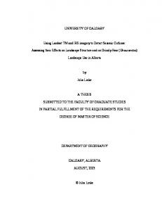
In order to describe the mathematical model of a discrete-time quantum walk, two quantum mechanical systems are needed, a quantum walker and a coin [23]. For a discrete-time quantum walk on a line Fig. 1.1, to every point j on the line we assign a quantum state |ji.
3
-4
-3
-2
-1
0
1
2
3
4
Figure 1.1: Discrete-time quantum walk on a line. Therefore the position Hilbert space of the walker Hp is spanned by basis states {|ji : j ∈ Z}. States of the discrete-time quantum walk live in H = Hp ⊗ Hc where Hc is the coin-space. For the case of a line the coin space Hc spanned by basis states {| ↑i, | ↓i}, the translation operator of the quantum walker can be written as S = | ↑ih↓ | ⊗
X
|j + 1ihj| + | ↓ih↑ | ⊗
X
j
|j − 1ihj|.
(1.1)
j
The Hadamard coin operator is an unbiased unitary coin with the following properties 1 CH | ↑i = √ (| ↑i + | ↓i) ; 2
(1.2a)
1 CH | ↓i = √ (| ↑i − | ↓i) . 2
(1.2b)
The evolution of the system in time from n to n + 1 can be written via a unitary operator in the following form: |Ψitn+1 = S.(CH ⊗ I)|Ψitn .
4
(1.3)
Although discrete-time quantum walks are quantum mechanical analogues of classical random walks, it has been shown that they have counterintuitive and fascinating behaviours. The limiting probability distribution of an unbiased classical discrete-time random walk on an infinite line approaches a Gaussian distribution with mean zero and variance σ 2 = Ns , where Ns is the number of steps. Nayak et al. [34] showed discrete-time quantum walks on a line with the Hadamard coin and a symmetric initial condition (|Ψ0 i =
√1 2
[| ↑i + ı| ↓i] ⊗ |0i)
does not approach a Gaussian distribution and more surprisingly σ 2 = Ns2 . Moreover Ambainis et al. [33] and Bach et al. [35] showed that the escaping probability of a quantum walker in a Hadamard walk on a line with an absorbing wall is not zero. The escaping probability in the classical case is zero and the walker will get absorbed by the wall. Discrete-time quantum walks are the subject of an active field of research, these examples being just the tip of the iceberg.
Continuous-time quantum walks are the quantum mechanical analogs of continuous-time classical Markov chains. They were first introduced by Farhi and Gutmann [36]. The main difference between this model and the discrete-time model is that the Hilbert space for the continuous-time case is Hp , the Hilbert space for the position of the walker, and there is no need for coin flipping or a coin unitary operator. In 2002, Childs et al. [37] defined a general formalism for continuous-time quantum walks on a graph. In this model the dynamic of the state is described via the time-dependent Schr¨odinger equation ı~
d |Ψi = H|Ψi, dt
(1.4)
where H is the Hamiltonian for the continuous-time quantum walk. He defined the Hamiltonian with the help of a probability generator matrix of a graph Mp . Continuous-time quantum walks will be introduced and discussed in more detail in the next chapter.
Quantum walks can be powerful algorithmic tools for designing and implementing quan5
tum algorithms. A quantum algorithm for finding a triangle in graph G [38, 39] and the graph collision problem [40] are interesting examples of quantum algorithms based on quantum walks. Refs. [23, 41, 42, 43, 44, 45] provide comprehensive reviews and introductions to quantum walk-based algorithms. All these algorithms follow a general recipe which consists of two important steps: I) Defining a suitable unitary operator for describing the time evolution of the system for the discrete case or an appropriate Hamiltonian for the continuous case. II) Finding a set of convenient measurement operators for finding the position of the quantum walker.
In 2003, the first connection between quantum walk-based algorithms and the quantum search algorithm was made by Shenvi et al. [46]. I quote a sentence from their article which shows the crucial role of this article in the history of quantum computation and quantum information: “However, previous to a very recent paper by Childs et al. [47], there had been no quantum algorithms based on the random walk model.” In this article Shenvi et al. used the discrete-time quantum walk as a quantum search algorithm on a hypercube [48, 49] with N = 2n vertices, where n is the dimension of the hypercube. They showed the searching time √ for this algorithm is O( N ). In other words they showed that this discrete-time quantum walk search algorithm can be a spatial simulation of Grover’s search algorithm.
Childs and Goldstone [50] developed a spatial search algorithm via continuous-time quantum walks based on the Farhi and Gutmann [36] continuous model. In this model they marked a vertex w on a graph G and they introduced the marking Hamiltonian as the projection operator of the state of a marked vertex Hw = |wihw|,
6
(1.5)
and they used the following Hamiltonian for describing the time evolution of the system H = −γL − |wihw|,
(1.6)
where γ is the hopping rate between two adjacent vertices of the graph G and L is the Laplacian of G. They showed that for a complete graph, hypercube and d-dimensional square lattice when d > 4, the search time for finding the the marked site w with this model √ is O( N ). For the complete graph with N vertices, the search time of this spatial search √ √ algorithm is O( N ), with the search time T = π2 N . They showed that when γ = N1 the probability of finding the quantum walker at the marked vertex w, at T is |hw|Ψ(T )i|2γ= 1 = 1.
(1.7)
N
In the next chapter I introduce their model with more details and reproduce the above results with a different mathematical approach.
Later in 2004 [51], by adding an additional degree of freedom and using the Dirac Hamiltonian they showed when d ≥ 3 quadratic speed-up is attainable and when d = 2 the √ searching time is O( N log N ). This new result perfectly matches the Ambainis et al. [52] discrete-time based algorithm.
Thus far, all the quantum walk algorithms I have reviewed in this introduction are run by a single quantum walker. If we substitute the single quantum walker by M identical non-interacting walkers for one of these algorithms, the results of the algorithm remain unchanged. Intuitively the problem of a quantum walk-based algorithm with M identical non-interacting quantum walkers is reducible to the problem of M separate identical algorithms with a single quantum walker. An immediate question that arises is then: what would happen if we substitute the single quantum walker with M indistinguishable interacting quantum walkers? In quantum mechanics, the only indistinguishable particles that 7
exist in nature are bosons and fermions. Boson wave functions do not have to be antisymmetrized; therefore, they do not satisfy the Pauli exclusion principle. Unlike fermions, there is no restriction on the number of bosons that can occupy a given site. For this reason, bosons are ideal candidates for this purpose. The goal of this research is to investigate the role of substituting the walker in a continuous-time quantum walk [50] by interacting bosons at zero temperature.
Bose-Einstein Condensation (BEC) was first introduced by Bose [53] and Einstein [54, 55], in 1924. Wolfgang Ketterle, Eric Cornell, and Carl Wieman first observed BEC in 1995, and won the Nobel prize for their work in 2001 [56, 57]. Due to a successful and promising series of experiments with trapped atoms, started by Anderson et al. [58] and Davis et al. [56], BEC has become one of the hottest topics in physics. There has been great theoretical and experimental effort in this field since then. Comprehensive reviews and introductions to BEC can be found in [59, 60, 61].
In 1947, Nikolay Bogoliubov [62, 63] developed a mathematical description for uniform weakly low-temperature Bose gases. In the early 1960s Gross [64, 65] and Pitaevskii [66] improved Bogoliubov’s model for nonuniform zero-temperature weakly interacting Bose gases. This extension yielded the celebrated Gross-Pitaevskii equation, also known as the non-linear Schr¨odinger equation ∂ ı~ ψ(~r, t) = ∂t
� 2 2 � ~∇ 2 − + Vext (~r) + g|ψ(~r, t)| ψ(~r, t), 2m
(1.8)
where 4π~2 as g= . m
(1.9)
Here m is the mass of the boson and as is the s-wave scattering length, a single parameter for characterizing the binary collisions at low energies and ~ is Planck’s constant. This equation describes the wave function of a Bose-Einstein condensate for a large number of bosons 8
at zero temperature. Note that ψ(r, t) is the single-particle quantum state occupied by M R atoms, and is therefore normalized as d~r|ψ(~r, t)|2 = M .
As mentioned in Eq. (1.8), the quantum mechanical model for interacting bosons at zero temperature is non-linear. The non-linear model is strictly valid at zero temperature. Therefore if we substitute the single quantum walker with interacting bosons at zero temperature, the continuous-time quantum walk model becomes non-linear. The question we want to address in this thesis is the following: is it possible to perform a quantum spatial search algorithm with this non-linear model? If so, it would immediately imply that physical systems with many interacting bosons could be useful for quantum computation. Non-linearity can also change the time scale of a dynamical system [67] which raises another crucial question: does this non-linearity change the scaling of search time of the algorithm?
This thesis is organized as follows. In Chapter 2 I introduce the Childs and Goldstone model [50]. I define the complete graph and its mathematical properties. I rederive their results for the case of a complete graph with a different mathematical approach. In Chapter 3 I use this approach as a basis for my calculations. In Chapter 3 I derive the Hamiltonian for interacting bosons in a discrete space and I define the mathematical model for a non-linear continuous-time quantum walk on a graph G. I apply this model to the complete graph. Using the symmetry of the complete graph, I reduce this problem to a two-dimensional non-linear problem. I also show it is possible to have a successful search (complete search) and quadratic speed-up is obtainable with this non-linear search algorithm. I conclude and discuss possible future directions in Chapter 4.
9
Chapter 2 Continuous-time quantum walk on a complete graph 2.1 Mathematical introduction In this section I introduce the Childs and Goldstone [50] continuous-time quantum walk algorithm in more detail. I reproduce the results of this model for a complete graph with N vertices. In order to achieve this goal I use a different mathematical approach. Later I use this method as a basis for solving the non-linear case. As shown in [50], the Hamiltonian for this model has the form H = −γL − Hw .
(2.1)
Here Hw is the marking Hamiltonian, Hw = |wihw|. This give the Hamiltonian the form H = −γL − |wihw|,
(2.2)
where γ is the hopping rate between two connected vertices in graph G, w is the marked vertex, and L is the Laplacian matrix for the graph G. I define the Laplacian matrix L = A− D. A is the adjacency matrix for G and it shows the connectivity of the graph as 1, (i, j) ∈ E Aij = . 0, otherwise
(2.3)
Graph G is defined as an ordered pair of two sets G = (V, E). V is a set of vertices and E is a set of edges. If the vertex i is adjacent to vertex j then (i, j) ∈ E. In this study I assume G is an undirected graph which means the edges have no specific direction. Therefore if (i, j) ∈ E then (j, i) ∈ E. D is the diagonal matrix with Dii = deg(i), the degree of a vertex i. The degree of vertex i
10
2
1
3
5 4
Figure 2.1: An arbitrary undirected graph G with 5 vertices and 7 edges. is defined as the number of vertices adjacent to i. For instance A and D, for the graph in Fig. 2.1, have the 3 0 1 0 1 1 0 1 0 1 0 1 A = 0 1 0 1 0 , D = 0 0 1 0 1 0 1 0 1 1 0 1 0
form 0 0 0 0 3 0 0 0 . 0 2 0 0 0 0 3 0 0 0 0 3
Therefore the Laplacian matrix takes the form: 0 1 1 −3 1 1 −3 1 0 1 L= 0 1 −2 1 0 1 0 1 −3 1 1 1 0 1 −3
(2.4)
.
(2.5)
In the next section I define the complete graph and I introduce some of its mathematical properties. 11
2.1.1 Mathematical properties of a complete graph In this section I define the complete graph and I review some of its mathematical properties such as the Laplacian and adjacency matrices and their eigenvalues and eigenstates. In graph theory a complete graph is a graph in which every pair of vertices is linked by a unique undirected edge. In graph theory a complete graph with N vertices is denoted by KN . Some sources claim that the letter K in this notation comes from the German word komplett. However there are some sources that claim the notation comes from Kazimierz Kuratowski’s name, because of his great contributions to graph theory. Fig. 2.2 shows the drawings of two complete graphs resulting when vertices are placed on a regular polygon. Such a graph is also known as a mystic rose. In the general case of KN , each vertex has N −1 neighbours; in other words, the graph is maximally connected. Therefore the complement of a complete graph is an empty graph. This maximal connectivity yields maximal accessibility for the complete graph which means every vertex is connected to every other vertex by one edge. Because of this property the complete graph can be used as the most ideal arrangement of a physical database.
2.1.2 Adjacency and Laplacian matrix Since the complete graph is fully connected, the adjacency matrix has a simple form. In this study I assume that the graph does not contain self loops, so that all the diagonal terms are
12
Figure 2.2: K8 and K20 , complete graphs with 8 and 20 vertices. zeros and the rest are one. This gives the adjacency 0 1 . 1 0 . . 1 . A=J −I = . . . . 1 1 .
matrix the form . . 1 . . 1 . , . . 0 1 . 1 0
(2.6)
where J is the all -1 matrix and I is the identity matrix. One can write the characteristic polynomial for the complete graph’s adjacency matrix in the form of PKN (λ) = (λ − N + 1)(λ + 1)N −1 .
(2.7)
If I set the characteristic polynomial to zero, it gives the eigenvalues or spectrum of the complete graph’s adjacency matrix. By solving PKN (λ) = 0 for λ, one obtains λ1 = −1 (N − 1 times) λ: , λ2 = N − 1 13
(2.8)
which shows that the adjacency matrix for KN without self-loops is (N − 1)-fold degenerate. In order to find the eigenvectors of the adjacency matrix for KN , one can write A in the following form: A = N |SihS| − I,
(2.9)
where I is the identity matrix and |Si is a normalized vector with the following form: 1 |Si = √ (1, 1, ..., 1)† . N
(2.10)
Therefore the corresponding normalized eigenvector for λ2 is |Si A|Si = N |SihS|Si − I|Si = (N − 1)|Si.
(2.11)
Since A is (N −1)-fold degenerate, the rest of the eigenvectors can be any (N −1)-dimensional set of orthogonal vectors which live in the hyper-surface defined by the normal vector |Si. Moreover, KN is a regular graph with degree N − 1, therefore D takes the following form: D = (N − 1)I,
(2.12)
where I is the identity matrix. Therefore the Laplacian matrix takes the following form: −(N − 1) 1 . . . 1 1 −(N − 1) . . . 1 . 1 . . . L=A−D = (2.13) . . . . . . . 1 1 1 . . 1 −(N − 1) Since the matrix D is a multiple of I, the Laplacian matrix has the same eigenvectors as the adjacency matrix and the spectrum of L is just a constant shift in the adjacency matrix’s spectrum, l:
l1 = −N
(N − 1 times)
l2 = 0 14
.
(2.14)
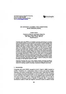
2.2 Continuous-time quantum walk on a complete graph In this section I want to solve the time-dependent Schr¨odinger equation under the Hamiltonian of Eq. 2.2 with |Si as the initial state. A complete search is a search in which the probability of finding the particle in the marked site or vertex approximately reaches one for some value of time T . Since the goal of the search algorithm is to find the marked vertex it should be a unique property of the marked vertex. T is called the hitting time or search time of the algorithm. As mentioned earlier, γ is the hopping rate between two adjacent vertices. This algorithm gives a high probability of finding the quantum walker in the marked vertex, for some value of γ called critical γ. As pointed out above, the adjacency and Laplacian matrices for the complete graph have only two distinct eigenvalues. This property suggests a symmetry which reduces our problem to a two-dimensional problem. As shown in Fig. 2.3, swapping two unmarked vertices i and j does not change the configuration of KN and furthermore, it keeps the Hamiltonian of the system unchanged. Since swapping two unmarked vertices does not change the Hamiltonian, one might expect that if the search starts in a uniform superposition of all vertices, all the unmarked vertices must have the same quantum state or in a more mathematical form ∀ i, j (i 6= w, j 6= w) ψi (t) = ψj (t), where ψi ≡ hi|ψi and ψj ≡ hj|ψi. Fig. 2.4 shows the numerical results of the spatial search on K8 based on the continuous-time quantum walk. As shown these results confirm this symmetry. However here I wish to prove this symmetry analytically. To accomplish the proof, I define the function ξij in the following form: ξji ≡ ψj (t) − ψi (t).
(2.15)
Therefore I can write the derivative of ξij with respect to time as ξ˙ji = ψ˙j − ψ˙ i .
15
(2.16)
j
i
i
j
w
w
Figure 2.3: Geometrical representation of the complete graph To find the ψ˙j , I use the time-dependent Schr¨odinger equation for the vertex j. Henceforth I assume ~ = 1, ıhj|
d |ψi = hj|(−γL − |wihw|)|ψi. dt
(2.17)
According to the definition of the Laplacian matrix, L|ji = (A − (N − 1)I)|ji =
N X
|mi − (N − 1)|ji =
N X
|mi − N |ji.
(2.18)
m=1
m6=j
By substituting this result into Eq. (2.17), ψ˙j takes the following form: N X
ψ˙j = −ı[−γ(
ψm − N ψj ) − δj,w ψw ].
(2.19)
m=1
By following the same procedure for ψi , one obtains ψ˙ i = −ı[−γ(
N X
ψm − N ψi ) − δi,w ψw ].
(2.20)
m=1
Therefore one can write ξ˙ji as follows ξ˙ji = −iγN (ψj − ψi ) + i(δj,w − δi,w )ψw . 16
(2.21)
Ψ7
Ψ
°Ψ2´ 2
°Ψ7´ 0.35
0.35
0.30
0.30
0.25
0.25
0.20
0.20
0.15
0.15
0.10
0.10
0.05
0.05
5
10
15
20
t
5
10
15
10
15
t
20
t
t
Ψ
Ψ
°Ψ3´ 3
°Ψ1´ 1
1.0
0.35
0.30 0.8 0.25 0.6 0.20
0.15
0.4
0.10 0.2 0.05
5
10
15
20
t 5
20
t
t
t
Figure 2.4: Continuous-time random walk on K8 , the amplitude of ψ1 , ψ2 , ψ7 and ψ3 with the marked vertex w = 3 and γ = 0.125.
17
Since i 6= w and j 6= w then δj,w = δi,w = 0, ξ˙ji takes the following form: ξ˙ji = −iγN ξji .
(2.22)
The general solution for this one-dimensional differential equation is ξji = Ce−iγN t ,
(2.23)
where C is a constant which will be determined by the initial condition. Since in this problem the initial state is the uniform superposition of all states 1 ψj (0) = ψi (0) = √ . N
(2.24)
ξji (0) = ψj (0) − ψi (0) = 0.
(2.25)
The initial condition for ξji is
By applying this initial condition to the general solution, one obtains ξji = 0.
(2.26)
Therefore one can write (i, j 6= w).
ψj = ψi
(2.27)
According to this symmetry, the continuous-time quantum walk on a complete graph is a two-dimensional problem. Therefore in order to describe the state of the system we need two independent parameters. Naturally one of these parameters is ψw and the other one is ψα , where α can be any number in the set of {1, 2, ..., w − 1, w + 1, ..., N } ψα ≡ ψ1 = ψ2 = ... = ψw−1 = ψw+1 = ... = ψN .
(2.28)
As shown in Eq. (2.9) and Eq. (2.12) the adjacency matrix can be written as A = N |SihS|−I and D = (N − 1)I. Therefore the Laplacian matrix for KN becomes L = N |SihS| − N I. 18
(2.29)
Since −N I creates a constant shift in energy levels and it does not change the dynamic of the system the Laplacian matrix can be changed to L → L + N I = N |SihS|,
(2.30)
where |Si is the initial state. Therefore the Hamiltonian takes the following form: H = −γN |SihS| − |wihw|.
(2.31)
The time-dependent Schr¨odinger equation for ψα and ψw can be written as follows d |ψi = hw|H|ψi = −γN hw|SihS|ψi − hw|ψi; dt
(2.32a)
d |ψi = hα|H|ψi = −γN hα|SihS|ψi − hα|wihw|ψi. dt
(2.32b)
ıhw|
ıhα|
Since |Si is the normalized uniform superposition of all the vertices, 1 hα|Si = hw|Si = √ . N
(2.33)
Using the symmetry of the complete graph, hS|ψi becomes N 1 X 1 1 hS|ψi = √ ψl = √ (ψ1 + ... + ψw−1 + ψw+1 + ... + ψN + ψw ) = √ [(N − 1)ψα + ψw ]. N l=1 N N (2.34)
Using these equations, the time-dependent Schr¨odinger equations for ψα and ψw become ıψ˙w = −(γ + 1)ψw − γ(N − 1)ψα ;
(2.35a)
ıψ˙α = −γψw − γ(N − 1)ψα ,
(2.35b)
or in a more compact form ˙ ψw γ + 1 γ(N − 1) ψw ψw ı = − ≡ Γ . ψ˙α γ γ(N − 1) ψα ψα 19
(2.36)
This equation describes a linear two-dimensional dynamical system. It is convenient to introduce a new variable as follows ψµ ≡
√
N − 1ψα ,
which allows us to rewrite equations (2.35) in an explicitly symmetric form as follows √ ıψ˙w = −(γ + 1)ψw − γ N − 1ψµ ;
(2.37a)
√ ıψ˙µ = −γ N − 1ψw − γ(N − 1)ψµ ,
(2.37b)
√ ˙ γ N − 1 ψw γ+1 ψw ı = − √ . ψ˙µ γ N − 1 γ(N − 1) ψµ
(2.38)
or more compactly
I define the matrix operator H2D √
γ N −1 γ+1 H2D ≡ − √ . γ N − 1 γ(N − 1)
(2.39)
The new initial state is
1 1 ψw (0) = √ √ . N N −1 ψµ (0)
(2.40)
Before solving this problem and finding the search time and critical γ, I would like to explain the physical meaning of ψµ and the geometrical interpretation of this two-dimensional Hamiltonian. Since H2D is Hermitian, the new two-dimensional quantum state (ψw , ψµ ), is normalized to one |ψµ |2 + |ψw |2 = 1.
(2.41)
According to the definition of ψw , |ψw |2 is the probability of finding the particle in the marked vertex w. Therefore |ψµ |2 is the probability of finding the particle in an unmarked vertex. In other words |ψµ |2 = |ψ1 |2 + |ψ2 |2 + ... + |ψw−1 |2 + |ψw+1 |2 ... + |ψN |2 . 20
(2.42)
Γ
N -1
Γ +1
Γ HN - 1L
w
Μ
Figure 2.5: Reduction of continuous-time quantum walk on KN to a two dimensional problem. Here, γ is the hopping rate and N is the dimension of the complete graph. As shown in Fig. 2.5, geometrically this symmetry reduces the continuous-time quantum walk on KN to a continuous-time quantum walk on a line with two vertices, with self loops and √ different hopping rate γ 0 = γ N − 1. For a large database (N � 1), the two dimensional Hamiltonian H2D becomes √ √ −(γ + 1) −γ N − 1 γ+1 γ N H2D = ≈ − √ . √ −γ N − 1 −γ(N − 1) γ N γN For the sake of simplicity, I define the following basis. 1 0 |wi = , |µi = . 0 1 In this regime, the initial state becomes 1 1 0 √ √ ≈ = |µi. N N −1 1
(2.43)
(2.44)
(2.45)
When N � 1, the eigenvalues of H2D , are p 1 E1 = − [1 + (N + 1)γ + (1 + (N + 1)γ)2 − 4N γ]; 2 21
(2.46a)
p 1 E2 = − [1 + (N + 1)γ − (1 + (N + 1)γ)2 − 4N γ]. 2
(2.46b)
In order to make the calculations easier I define p α ≡ 1 + (N + 1)γ, β ≡ (1 + (N + 1)γ)2 − 4N γ, √ ζ ≡ 1 − (N − 1)γ, κ ≡ 2γ N . Therefore the eigenvalues become 1 E1 = − (α + β); 2
(2.47a)
1 E2 = − (α − β), 2
(2.47b)
and the eigenvectors are
1 ζ +β |E1 i = p ; (ζ + β)2 + κ2 κ |E2 i = p
(2.48a)
ζ −β . (ζ − β)2 + κ2 κ 1
(2.48b)
Since |E1 i and |E2 i are the eigenvectors of H2D , they are orthogonal hE1 |E2 i = ζ 2 − β 2 + κ2 = 0
=⇒ κ2 = β 2 − ζ 2 ,
(2.49)
which yields
1 ζ +β |E1 i = p ; 2β(ζ + β) κ
(2.50a)
1 ζ −β |E2 i = p . 2β(β − ζ) κ
(2.50b)
The solution of the time-dependent Schr¨odinger equation has the following form: |ψ(t)i = c1 |E1 ie−ıE1 t + c2 |E2 ie−ıE2 t , 22
(2.51)
where ci = hEi |ψ(0)i. Since the initial state is |µi for large N , c1 and c2 take the following form: κ ; c1 = hE1 |µi = p 2β(ζ + β)
(2.52a)
κ c2 = hE2 |µi = p . 2β(β − ζ)
(2.52b)
2.2.1 Finding the critical γ The objective of this section is to find the critical value of γ, called γ ∗ , that satisfies the following condition |ψw (T )|2 ≈ 1,
(2.53)
where T is the search time for this algorithm. As pointed out in the previous section, the solution of the time-dependent Schr¨odinger equation is the following κ 1 ζ + β i (α+β)t 1 ζ − β i (α−β)t − |ψ(t)i = e2 e2 . 2β ζ + β ζ −β κ κ
(2.54)
Therefore the quantum state for the marked site takes the following form: i
ψw (t) = e 2 αt
i κ i βt (e 2 − e− 2 βt ), 2β
(2.55)
where ψw (t) = hw|ψ(t)i. The amplitude of ψw (t) is κ β | sin( t)| β 2 κ =⇒ 0 ≤ |ψw (t)| ≤ . β |ψw (t)| =
23
(2.56)
Κ Β 1.0
0.8
0.6
0.4
0.2
0.0005
0.0010
0.0015
0.0020
Γ
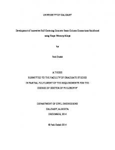
Figure 2.6: The maximum of |ψw | as a function of γ, for N = 1024. By substituting κ and β in the above equation I obtain the following equation for the maximum of |ψw (t)| |ψw (t)|max
√ κ 2γ N = =p . β (1 + (N + 1)γ)2 − 4N γ
(2.57)
As shown in Fig. 2.6 at some value of γ the maximum value for |ψw | reaches one. To obtain the critical value of γ, one can solve the following equation for γ √ 2γ N d [p ] = 0, dγ (1 + (N + 1)γ)2 − 4N γ
(2.58)
hence √ 2 N [1 − (N − 1)γ] 3
[(1 + γ(N + 1))2 − 4N γ] 2
= 0.
(2.59)
It is straightforward to show that the critical γ, γ ∗ , is γ∗ =
1 . N −1
For a large database (N � 1), it becomes γ ∗ ≈
1 . N
(2.60)
Therefore when γ = γ ∗ , the continuous-
time quantum walk search algorithm on a complete graph provides a complete search. In 24
other words for a large database at critical γ |ψw (T )|2 ≈ 1,
(2.61)
where T is the search time for this algorithm.
2.2.2 Time scale and search time In the previous section I showed that ψw (t) has the following form: i
ψw (t) = e 2 αt
i κ i βt (e 2 − e− 2 βt ). 2β
(2.62)
i
Since e 2 αt is an overall phase factor, I can write |ψw (t)| in the following form: |ψw (t)| =
i i κ κ β |(e 2 βt − e− 2 βt )| = | sin( t)|, 2β β 2
(2.63)
p √ where κ = 2γ N and β = (1 + (N + 1)γ)2 − 4N γ. At critical γ, β and κ take the following form: √
β|γ=γ∗ =
p
(1 + (N + 1)γ)2 − 4N γ|γ=
=2
N 2 ≈√ ; N −1 N
(2.64a)
√
√
κ|γ=γ ∗ = 2γ N |γ=
1 N −1
1 N −1
=2
N 2 ≈√ . N −1 N
Substituting β from the above equations into |ψw (t)|, one obtains √ N |ψw (t)| = | sin( t)|. N −1
(2.64b)
(2.65)
For a large database (N � 1), |ψw (t)| takes the following form: t |ψw (t)| = | sin( √ )|. N 25
(2.66)
Ψw
2
1.0
0.8
0.6
0.4
0.2
20
40
60
80
100
120
140
t
Figure 2.7: Probability of finding the particle at the marked site, |ψw |2 as a function of time, for N = 1024 and γ = N1 . |ψw | reaches one when T ≈
π√ N, 2
(2.67)
consistent with the results shown in Fig. 2.7. Therefore the continuous-time quantum walk on a complete graph provides quadratic speed-up over a classical search.
26
Chapter 3 Non-linear continuous-time quantum walk In the previous chapter I showed that spatial search via a continuous-time quantum walk with one quantum walker on a complete graph provides a quadratic speed up over a classical search. In this chapter I construct a model for continuous-time quantum walks on a graph G with interacting bosonic walkers at zero temperature and show that the Hamiltonian for this system has the form HN L = −γL − |wihw| + g
N X
|ψi |2 |iihi|,
(3.1)
i=1
where γ is the hopping rate, L is the Laplacian matrix, w is the marked site, g is the interaction coefficient, and ψi = hi|ψi. The central questions to be addressed in this Chapter are first: Is it possible to perform a complete quantum search with many interacting bosons on a spatial database? In other words, is it possible to rotate the initial state |Si to the desired state |wi, with this non-linear Hamiltonian for some values of γ and g? Second: If it is possible, what is the time scale for this process? It has been show that for some cases non-linearity can change the time scale of a dynamical system [67]. Can non√ linearity change the time scale of the search algorithm, or is it still proportional to N and hence quadratic speed-up is attainable? In order to address these questions I use non-linear dynamics techniques that include fixed point analysis, linearization at fixed points, stability analysis and phase space analysis. I review the basics of these techniques in Appendix A. I use fixed point analysis and linearization techniques to find the regimes of g and γ that provide a complete quantum search algorithm. I use phase space analysis for finding the time scale for the search algorithm.
27
3.1 Interacting bosons at zero temperature as quantum walkers As mentioned in the introduction, the goal of this research is to investigate the spatial search via a continuous-time quantum walk with interacting bosons at zero temperature. In this section I derive the Hamiltonian for interacting bosons at zero temperature in a discrete space such as a graph or a lattice. When there are a large number of bosons, the fluctuations in the number of bosons is negligible and a mean field approach is valid [60]. In the second quantization the many-body Hamiltonian describing M interacting bosons in an external potential Vext has the following form [59]: � � Z ~2 2 † ˆ ˆ H = drΨ (r) − ∇ + Vext (r) Ψ(r) 2m Z 1 ˆ † (r)Ψ ˆ † (r0 )V (r − r0 )Ψ(r ˆ 0 )Ψ(r), ˆ + drdr0 Ψ 2
(3.2)
ˆ ˆ † (r) are boson field annihilation and creation operators, and V (r − r0 ) is where Ψ(r) and Ψ the two-body interatomic potential. For a discrete space such as a graph or lattice, I can write the Hamiltonian for interacting bosons in the following form: Hint =
1 XX ˆ† ˆ † (rj )V (ri − rj )Ψ(r ˆ j )Ψ(r ˆ i ), Ψ (ri )Ψ 2 i j
(3.3)
where ri and rj are the position vectors of the vertices i and j in graph G. By writing the Heisenberg equation for the interaction part of the Hamiltonian, one can prove that (below ~ = 1 as was assumed in the previous chapter) " # X ˆ i) ∂ Ψ(r † ˆ (rj )V (rj − ri )Ψ(r ˆ j ) Ψ(r ˆ i ). = ı Ψ ∂t j
(3.4)
ˆ i) = Ψ ˆ i . At zero temperature, when BEC occurs, the Bogoliubov [59] first-order I define Ψ(r approximation can be used ˆ i = Ψi + Ψ ˆ 0, Ψ i
(3.5)
where Ψi is a complex function defined as the expectation value of the field operator ˆ i i. Ψi = hΨ 28
(3.6)
ˆ 0 can be treated as a very small perturbation [59]. When BEC is macroscopically occupied, Ψ i Therefore Eq. (3.4) takes the following form: ı
!
∂Ψi ≈ ∂t
X
Ψ∗j Vij Ψj
Ψi .
(3.7)
j
Rewriting the above equation in the following form: X ∂ ıhi| |Ψi = hi| Ψ∗j Vij Ψj ∂t j
! |Ψi,
(3.8)
gives Hint =
XX i
By defining Ψi =
√
Ψ∗j Vij Ψj |iihi|.
(3.9)
j
M ψi , where M is the number of bosons in the system, one can write the
Hamiltonian for the interaction in the following form: Hint = M
XX i
ψj∗ Vij ψj |iihi|.
(3.10)
j
Since in a cold and dilute boson gas, binary collisions at low energy are the dominant interactions [60], one can approximately replace Vij by Vij = gδij ,
(3.11)
4πas , m
(3.12)
where g [59] g=
where m is the mass of the boson and as is the s-wave scattering length, a single parameter for characterizing the binary collisions at low energies. This parameter is independent of the details of Vij . Therefore Hint = g
N X i=1
29
|ψi |2 |iihi|.
(3.13)
Note that X
|Ψi |2 = M
−→
i
X
|ψi |2 = 1,
(3.14)
i
where ψi = hi|ψi and N is the number of sites in the graph G.
3.2 Reduction to a two-dimensional problem As pointed out earlier, the non-linear Hamiltonian for a continuous-time quantum walk with bosonic interacting quantum walkers has the following form: Hnl = −γL − |wihw| + Hint ,
(3.15)
therefore Hnl = −γL − |wihw| + g
N X
|ψi |2 |iihi|,
(3.16)
i=1
where nl stands for non-linear, ψi = hi|ψi and |ii is the ket representing the vertex i. The Laplacian matrix for the complete graph can be written N |SihS|, so that in case of the complete graph, Eq. (3.16) becomes Hnl = −γN |SihS| − |wihw| + g
N X
|ψi |2 |iihi|.
(3.17)
i=1
This Hamiltonian is N -dimensional; however the question is, can I reduce this non-linear Hamiltonian to a two-dimensional Hamiltonian with the complete graph’s symmetry? Similar to the linear since swapping the unmarked vertex i with another unmarked vertex j in KN keeps the Hamiltonian unchanged ψ1 = ψ2 = ... = ψw−1 = ψw+1 = ... = ψN . 30
(3.18)
The time-dependent Schr¨odinger equation for an arbitrary unmarked vertex α can be written as follows hα|ı
Hnl |ψi =
d |ψi = hα|Hnl |ψi, dt
−γN |SihS| − |wihw| + g
N X
(3.19)
! |ψi |2 |iihi| |ψi
i=1
√
= −γ N
N X
! ψi
|Si − ψw |wi + g
i=1
N X
|ψi |2 ψi |ii.
(3.20)
i=1
The right side of Eq. (3.19), becomes N N X √ X ψi )hα|Si − ψw hα|wi + g |ψi |2 ψi hα|ii. hα|Hnl |ψi = −γ N ( i=1
(3.21)
i=1
Since |Si is the uniform superposition of all the vertices and it is normalized to one, hα|Si = 1 . N
α is an unmarked vertex, hα|wi = δα,w = 0. Eq. (3.21) takes the following form: hα|Hnl |ψi = −γ
N X
ψi + g|ψα |2 ψα .
(3.22)
i=1
The goal of this section is to reduce this system to a two-dimensional system. In order to achieve this goal the right side of Eq. (3.22) should be expressed in terms of two variables, for instance ψw and ψα . Using the complete graph symmetry, Eq. (3.18) N X
ψi = ψ1 + ψ2 + ... + ψw−1 + ψw+1 + ... + ψN + ψw = (N − 1)ψα + ψw .
(3.23)
i=1
The time-dependent Schr¨odinger equation for the vertex α becomes ıψ˙α = −γ(N − 1)ψα − γψw + g|ψα |2 ψα .
(3.24)
Eq. (3.24) expresses the ψ˙α , in terms of two complex variables ψα and ψw . The timedependent Schr¨odinger equation for the marked vertex w hw|ı
d |ψi = hw|Hnl |ψi. dt 31
(3.25)
The right side Eq. (3.25) can be written as hw|Hnl |ψi = −γ
N X
ψi − ψw + g|ψw |2 ψw .
(3.26)
i=1
Using the complete graph symmetry, I can rewrite Eq. (3.26) as follows ıψ˙w = −γ(N − 1)ψα − (γ + 1)ψw + g|ψw |2 ψw .
(3.27)
Eq. (3.27) expresses ψ˙w , in terms of ψw and ψα . Therefore Eq. (3.24) and Eq. (3.27) describe a two-dimensional system of non-linear differential equations with complex variables. ıψ˙w = −γ(N − 1)ψα − (γ + 1)ψw + g|ψw |2 ψw ;
(3.28a)
ıψ˙α = −γ(N − 1)ψα − γψw + g|ψα |2 ψα .
(3.28b)
Equations (3.28), can be written more compactly in matrix form as 2 ˙ γ(N − 1) ψw ψw γ + 1 − g|ψw | ψw ı , (3.29) ≡ Γnl = − ψα ψα γ γ(N − 1) − g|ψα |2 ψ˙α with the initial condition
1 1 ψw (0) = √ . N ψα (0) 1
(3.30)
Although Eq. (3.29) perfectly describes the dynamics of the system, it is again convenient to introduce a new variable as follows ψµ ≡
√
N − 1ψα ,
(3.31)
which allows us to rewrite equations (3.28) in a symmetric form as follows √ ıψ˙w = −γ N − 1ψµ − (γ + 1)ψw + g|ψw |2 ψw ; √ ıψ˙µ = −γ N − 1ψw − γ(N − 1)ψµ + 32
g |ψµ |2 ψµ . N −1
(3.32a)
(3.32b)
In a more compact form, this is
˙ ψw ψw ı = H2Dnl , ψ˙µ ψµ
(3.33)
where H2Dnl has the following form: √ 2 γ N −1 γ + 1 − g|ψw | H2Dnl = − , √ γ N −1 γ(N − 1) − Ng−1 |ψµ |2 with the new initial condition
(3.34)
1 1 ψw (0) = √ √ . N ψµ (0) N −1
(3.35)
For a large spatial database N � 1, equations (3.32) take the following form: √ iψ˙w ≈ −γ N ψµ − (γ + 1)ψw + g|ψw |2 ψw , √ g iψ˙µ ≈ −γ N ψw − γN ψµ + |ψµ |2 ψµ , N
(3.36)
with initial state as
ψw (0) 0 ≈ . 1 ψµ (0) The non-linear Hamiltonian is then 2
γ + 1 − g|ψw | H2Dnl ≈ − √ γ N
33
(3.37)
√
γ N γN −
g |ψµ |2 N
.
(3.38)
3.3 Non-linear dynamics techniques and analysis Since equations (3.32) are expressed in terms of complex variables ψµ and ψw , this system is a two-dimensional system in the field of complex numbers. Each of these variables can be therefore represented by a real-valued phase and modulus. Therefore in the field of real numbers, it is a four-dimensional system of differential equations. On the other hand, since this system describes a two-dimensional quantum mechanical problem the solutions satisfies the following constraints I) The quantum state (ψw , ψµ ) is always normalized to one |ψµ |2 + |ψw |2 = 1.
(3.39)
II) If (ψw (t), ψµ (t)) is a solution of equations (3.32), then eıδ (ψw (t), ψµ (t))
∀δ ∈ R,
is also a solution of equations (3.32). Applying these constraints reduces this system to a two-dimensional system of differential equations, in the field of real numbers. In the following section my objective is to find appropriate variables that reflect these constraints and reduce this system to two real nonlinear differential equations.
3.3.1 Reduction to a real two-dimensional problem As mentioned above, ψw and ψµ can be presented by a real-valued phase and modulus as follows ψw ≡
p Nw eıθw ; 34
(3.40a)
ψµ ≡
p Nµ eıθµ ,
(3.40b)
where Nw is the fractional population of the bosons in the marked vertex w and Nµ is the sum of the fractional populations in all the unmarked vertices. Since (ψw , ψµ ) is normalized to one, one can write |ψw |2 + |ψµ |2 = Nw + Nµ = 1.
(3.41)
The best candidate for the first variable is the fractional population difference between the marked vertex w and the effective unmarked vertex µ, defined as follows [68] η ≡ Nw − Nµ .
(3.42)
The second variable must be invariant under the following transformation Φ : (θw , θµ ) =⇒ (θw + δ, θµ + δ).
(3.43)
The second variable is defined by the following form: φ ≡ θw − θµ .
(3.44)
In order to find the differential equation for η, start with the definition of η η = Nw − Nµ = |ψw |2 − |ψµ |2 = ψw ψw∗ − ψµ ψµ∗ .
(3.45)
The derivative of η with respect to time becomes η˙ = (ψ˙w ψw∗ + ψw ψ˙w∗ ) − (ψ˙µ ψµ∗ + ψµ ψ˙µ∗ ).
(3.46)
From equations (3.36), ψ˙w and ψ˙µ have the following form: ψ˙w = −ı[(ew + uw Nw )ψw − κψµ ];
(3.47a)
ψ˙µ = −ı[(eµ + uµ Nµ )ψµ − κψw ],
(3.47b)
35
where ew = −(γ + 1);
uw = g;
eµ = −γN,
uµ =
g , N
(3.48a)
(3.48b)
√ κ = γ N.
(3.48c)
ψ˙w∗ = ı[(ew + uw Nw )ψw∗ − κψµ∗ ];
(3.49a)
ψ˙µ∗ = ı[(eµ + uµ Nµ )ψµ∗ − κψw∗ ].
(3.49b)
Note that
With the help of equations (3.47) and (3.49) the first part of the right side of Eq. (3.46) becomes ψ˙w ψw∗ + ψw ψ˙w∗ = ıκ(ψµ ψw∗ − ψw ψµ∗ ),
(3.50)
and the second part takes the following form: ψ˙µ ψµ∗ + ψµ ψ˙µ∗ = −ıκ(ψµ ψw∗ − ψw ψµ∗ ).
(3.51)
Therefore η˙ takes the following form: η˙ = 2iκ(ψµ ψw∗ − ψw ψµ∗ ).
(3.52)
Substituting equations (3.40) into this equation we obtain p η˙ = 2ıκ(ψµ ψw∗ − ψw ψµ∗ ) = 2ıκ Nw Nµ [e−i(θw −θµ ) − ei(θw −θµ ) ] p = 4κ Nw Nµ sin(φ). Using the first constraint of the system,
(3.53)
p Nw Nµ becomes
q p 1 1p Nw Nµ = (Nw + Nµ )2 − (Nw − Nµ )2 = 1 − η2. 2 2 36
(3.54)
Therefore Eq. (3.53) becomes p η˙ = 2κ 1 − η 2 sin(φ).
(3.55)
This equation is the first real non-linear differential equation. In order to find the second one that expresses φ˙ in terms of η and φ, let ψw ψµ∗ =
p Nw Nµ ei(θw −θµ ) .
(3.56)
Substituting Eq. (3.54) into Eq. (3.56), one obtains ψw ψµ∗ =
1p 1 − η 2 eiφ . 2
(3.57)
Taking the derivative of both sides of this equation with respect to time η η˙ ıφ˙ p ψ˙w ψµ∗ + ψw ψ˙µ∗ = (− p + 1 − η 2 )eiφ . 2 2 2 1−η
(3.58)
Substituting Eq. (3.55) into the left side of Eq. (3.58) I obtain the following equation ! ıφ˙ p η η˙ + 1 − η 2 eiφ − p 2 2 2 1−η ! ıφ˙ p = −κη sin(φ) + 1 − η 2 eiφ . (3.59) 2 Using Equations (3.47) and (3.49) the left side of Eq. (3.58) takes the following form: p ψ˙w ψµ∗ + ψw ψ˙µ∗ = −ıκ(Nw − Nµ ) + ı[(eµ − ew ) + (uµ Nµ − uw Nw )] Nw Nµ eiφ .
(3.60)
With the help of the first constraint uµ Nµ − uw Nw =
uµ − uw uµ + uw − (Nw − Nµ ), 2 2
(3.61)
one obtains �
ψ˙w ψµ∗ + ψw ψ˙µ∗ = −ıκη + ı (eµ − ew ) +
�
uµ − uw 2
37
�
� −
uµ + uw 2
� �p 1 − η 2 iφ η e . 2
(3.62)
Therefore ! ıφ˙ p −κη sin(φ) + 1 − η 2 eiφ 2 � � � � � �p 1 − η 2 iφ uµ − uw uµ + uw = −ıκη + ı (eµ − ew ) + − η e . 2 2 2
(3.63)
Solving this equation for φ˙ yields the second non-linear differential equation uµ − uw uµ + uw η φ˙ = (eµ − ew ) + − η − 2κ p cos(φ). 2 2 1 − η2
(3.64)
Equations (3.55) and (3.64) describe a two-dimensional system in the field of real numbers. These equations also satisfy all the constraints of the original system. Therefore the nonlinear continuous-time quantum walk on the complete graph KN is reducible to a twodimensional system with real-valued variables as follows √ p η˙ = 2γ N 1 − η 2 sin(φ);
(3.65a)
√ g η φ˙ = ∆E − η − 2γ N p cos(φ), 2 1 − η2
(3.65b)
g ∆E ≡ 1 − N γ − . 2
(3.66)
where
According to the definition of η the initial value is η0 = |ψw (0)|2 − |ψµ (0)|2 =
2−N ≈ −1. N
(3.67)
Since the initial values for ψµ and ψw are real positive numbers, the initial condition of this new system is
η(0) = φ(0)
38
2−N N
0
.
(3.68)
Therefore for a large database (N�1) η(0) −1 ≈ . φ(0) 0
(3.69)
3.4 First regime: ∆E = 0 The goal in this section is to solve equations (3.65) when ∆E = 0. Setting ∆E equal to zero and solving for γ gives γ∗ =
2−g . 2N
(3.70)
Since γ is the hopping rate it should be always positive, therefore γ∗ > 0
→ g < 2.
(3.71)
In this regime Equations (3.65) take the following form: √ p η˙ = 2γ ∗ N 1 − η 2 sin(φ);
(3.72a)
√ g η φ˙ = − η − 2γ ∗ N p cos(φ). 2 1 − η2
(3.72b)
The first step for analyzing this system is to find the fixed points of Equations (3.72). As I defined in Appendix A, fixed points are the points in phase space satisfying the following equations η˙ ≡ 0;
(3.73a)
φ˙ ≡ 0.
(3.73b)
39
Fixed points provide qualitative information about the behaviour of the system. I discuss this in more detail in the following next section.
3.4.1 Fixed points In order to find the fixed points, I solve the following equations simultaneously √ p 2γ ∗ N 1 − η 2 sin(φ) ≡ 0;
(3.74a)
√ η g cos(φ) ≡ 0. − η − 2γ ∗ N p 2 1 − η2
(3.74b)
Solving the above equations yields two sets of fixed points as listed below I) The first set, as shown in Fig. 3.1, has the following form: η0 = 0,
φ = 2mπ
m ∈ Z.
II) The second set, as shown in Fig. 3.2, has the following form: q 4(g−2)2 η = + 1 − + g2 N , φ= (2m + 1)π m ∈ Z. η0 = 0 q η = − 1 − 4(g−2)2 − g2 N
(3.75)
(3.76)
The second set of fixed points η+ and η− are functions of g, in contrast to the first set. As shown in Fig. 3.3 η+ and η− become equal to zero for some value of g as follows g∗ = √
4 4 ≈√ . N +2 N
(3.77)
As shown in Fig. 3.3, η+ and η− , approach zero as g decreases and they become imaginary when g is smaller than the critical value. Furthermore as g increases they take the following 40
Η 1.0
0.5
-4
2
-2
4
Φ Π -0.5
-1.0
Figure 3.1: First set of fixed points for Equations (3.72).
Η
0.5
-3
-2
1
-1
2
3
Φ Π -0.5
Figure 3.2: Second set of fixed points for Equations (3.72), for N = 1024 and g = 0.125. Blue dots represent η+ , red dots represent η− and black dots represent η0 .
41
Η 1.0
0.5
0.5
1.0
1.5
2.0
g
-0.5
-1.0
Figure 3.3: Second set of fixed points for Equations (3.72) as a function of g, for N = 1024. The blue graph is η+ , the red one is η− and the black is η0 . form: lim η± = ±1.
g→∞
(3.78)
For the limiting case of strong on-site interactions (g � 1), intuitively there are three possible stationary states that particles tend to occupy. The first one is when they all accumulate in the marked vertex (η = +1), the second one is when they all accumulate in the effective unmarked vertex µ, (η = −1). The third one is when half of the particles are in the vertex w and the other half are in the vertex µ, (η = 0).
42
3.4.2 Classical Hamiltonian Although Equations (3.72) describe a quantum mechanical system, they can describe a classical system with the Hamiltonian HC satisfying the following equations [69] η˙ = −
∂HC ; ∂φ
∂HC φ˙ = . ∂η
(3.79a)
(3.79b)
It is not difficult to verify that this classical Hamiltonian has the following form: √ p g HC = − η 2 + 2γ ∗ N 1 − η 2 cos(φ). 4
(3.80)
As we know from classical mechanics, the dynamics of a quantity u can be written in the following form: du ∂u = {u, HC } + , dt ∂t
(3.81)
where {u, HC } is the Poisson bracket of u and HC . This equation also holds for HC , therefore H˙ C becomes dHC ∂HC = {HC , HC } + . dt ∂t
(3.82)
Since {HC , HC } = 0 and the classical Hamiltonian is not an explicit function of time the above equation becomes dHC = 0, dt
(3.83)
which shows that the classical Hamiltonian HC is a constant of motion. Eq. (3.83) shows that system is conservative, therefore I can use the theorem of Section A.2.3 for describing the behaviour of the trajectories near the fixed points.
43
3.4.3 Linearization near fixed points and stability analysis The goal of this section is to analyze the stability of the fixed points introduced in Section 3.4.1. For this analysis I use the method introduced in Section A.2.1. In order to linearize the system near the fixed points I construct the Jacobian matrix. As shown in Appendix A, the Jacobian matrix has the following form: J = In this problem the Jacobian matrix is J =
∂f ∂u
∂f ∂v
∂g ∂u
∂g ∂v
∂f ∂η
∂f ∂φ
∂g ∂η
∂g ∂φ
.
(3.84)
,
(3.85)
(u∗ ,v ∗ )
(η ∗ ,φ∗ )
where √ p f (η, φ) = 2γ ∗ N 1 − η 2 sin(φ);
(3.86a)
√ g η g(η, φ) = − η − 2γ ∗ N p cos(φ). 2 1 − η2
(3.86b)
Therefore
∗
√
∗
√
2
−2γ N η sin(φ) 2γ N (1 − η ) cos(φ) 1 √ J=p . √ √ g 1−η 2 2γ ∗ N cos(φ) ∗ 1 − η2 − 2 − 2γ N η sin(φ) 1−η 2 For the first set of fixed points the Jacobian matrix becomes √ ∗ 0 2γ N J(0,2mπ) = . √ − g2 − 2γ ∗ N 0 When N � 1 the eigenvalues of J have the following form: s √ (2 − g)(g N + 4) α± = ±i . 2N
44
(3.87)
(3.88)
(3.89)
Since the system is conservative, they are marginally stable or centers. As shown in Fig. 3.4 and Fig. 3.5 near these points trajectories circulate around them and eventually return to the initial point. Since the system is conservative the trajectories become closed trajectories or closed orbits.
For the second set of fixed points 2.a) For [η = 0, φ = (2m + 1)π] the Jacobian matrix takes the following form: J[0,(2m+1)π] =
−2γ
0 √ − g2 + 2γ ∗ N
∗
√
0
N .
When N � 1, the eigenvalues of J have the following form: s √ (2 − g)(g N − 4) . α± = ± 2N
(3.90)
(3.91)
There are two possible cases for the stability of these fixed points: 2.a.I) When
√4 N
√4 N
In this case the eigenvalues are both imaginary, therefore it is a marginally stable fixed point or a center. 2.b.II) When g ≤
√4 N
as mentioned earlier, when g ≤
√4 , N
η+ becomes imaginary and in this regime [η+ , (2m+1)π]
does not exist, therefore it is not a fixed point.
2.c) For [η = η− , φ = (2m + 1)π], the Jacobian matrix takes the following form: √ p ∗ 2 0 −2γ N 1 − η− J[η− ,(2m+1)π] = . √ ∗ − g2 + 2γ N3 0
(3.94)
(1−η− ) 2
Following the same procedure the eigenvalues of J are the same as in the previous case r 1 (N − 4)g 2 + 16g − 16 α± = ± − . (3.95) 2 N The only difference between this case and the previous one is that the trajectories near the η− , flow in the opposite direction near η+ . Figures 3.4 and 3.5 show the phase configuration and stability of fixed points in η − φ space for both regimes of g.
3.4.4 Phase space analysis In this section I analyze the phase space (η − φ space) with the help of the results obtained in previous sections. Phase space analysis helps to describe qualitative behaviour of the 47
solutions of Eq. (3.72) for different regimes of g. Moreover, with this analysis one can find conditions that provide a complete search η(T ) ≈ 1.
(3.96)
As mentioned in Section 3.4.2, the classical Hamiltonian HC √ p g HC = − η 2 + 2γ ∗ N 1 − η 2 cos(φ), 4 is a constant. With the following initial condition η(0) −1 = , φ(0) 0
(3.97)
(3.98)
the classical Hamiltonian has the following value g HC = HC [η(0), φ(0)] = − . 4
(3.99)
According to the definition of η, η = |ψw |2 − |ψµ |2 , the search is complete when η reaches one. Therefore the goal of my project is to find g and γ in such a way that the following transition happens (η = −1) −→ (η = +1).
(3.100)
The classical Hamiltonian is an even function of η, therefore Hc (η = −1, φ = 0) = Hc (η = +1, φ = 0).
(3.101)
The above equation reduces the problem to one of finding a closed orbit in phase space with (η = −1, φ = 0) as the initial condition. As mentioned earlier, when ∆E = 0, there are two possible regimes for g
γ∗ =
g > g∗
2−g , 2N
g ≤ g∗ 48
,
(3.102a)
Η 1.0
0.5
0.5
1.0
1.5
2.0
vÓ2
vÓ1
Φ Π
-0.5
-1.0
Figure 3.6: Qualitative analysis of the phase space for the first regime, g > g ∗ .
Η 1.0
0.5
1
2
3
4
5
Φ Π
-0.5
-1.0
Figure 3.7: The trajectory in η − φ space when g = 2g ∗ and γ = γ ∗ .
49
where g ∗ =
√4 . N
In the first regime g > g ∗ , as shown in Fig. 3.6, the trajectory starts at initial point (η = −1, φ = 0), then : I) The fixed point at (η = 0, φ = π) attracts the trajectory along v~1 . II) The trajectory flows clockwise around (η = η− , φ = π). III) (η = 0, φ = π) repels the trajectory along v~2 to the point (η = −1, φ = 2π). Therefore the trajectory never reaches η = +1. This regime does not provide a closed orbit. Fig. 3.7 shows the numerical solution for the trajectory in phase space when g = 2g ∗ . As mentioned in the previous section, in the second regime g ≤ g ∗ the stability of the fixed point (η = 0, φ = π) changes from an unstable saddle to a centre and the fixed points (η = η± , φ = π) vanish. As shown in Fig. 3.8, in this case the nearest fixed point to the initial point is at (η = 0, φ = 0) and is a centre; also the next nearest fixed points (η = 0, φ = ±π) are centres. Therefore the trajectory cannot be attracted by those points. Hence in this regime, as shown in Fig. 3.8, the trajectory starts from the initial point (η = −1, φ = 0), rotates around the origin, and reaches the final point of the search (η = 1, φ = 0). Since the trajectory is closed it comes back to the initial point. As shown in Fig. 3.9, the following regime γ = γ∗ =
2−g , 2N
4 g = g∗ = √ , N
(3.103)
provides a closed trajectory in the (η − φ) space. In other words, a complete search is attainable. For any g ∈ [0, √4N ] a complete search is attainable. For the sake of simplicity, henceforth, I assume 4 g = g∗ = √ . N
50
(3.104)
Η
Η
Η
1.0
1.0
1.0
0.5
0.5
0.5
0.2
-0.2
0.4
0.6
0.8
1.0
Π
Φ
Φ
Φ -0.4
0.5
-0.5
1.0
0.5
-0.5
Π
-0.5
-0.5
-0.5
-1.0
-1.0
-1.0
Figure 3.8: The closed trajectory in η − φ space when N = 1024 and γ = γ ∗ . The left graph ∗ is for g = 0, for the middle one is for g = g2 = √2N and the right one is for g = g ∗ = √4N . Η 1.0
0.5
20
40
60
80
100
120
t -0.5
-1.0
Figure 3.9: η as a function of time for N = 1024, when g = g ∗ and γ = γ ∗ . 51
1.0
Π
1.0
Η
0.5
0.5
-0.5
1.0
ΦΠ
-0.5
-1.0
Figure 3.10: Trajectory in η − φ space , for γ =
2−g , 2N
g=
√4 N
and N = 1024.
3.4.5 Time scale of the search algorithm As mentioned above, in the following regime ∆E = 0;
(3.105)
4 g = g∗ = √ , N a complete search is attainable: |ψw |2 (T ) ≈ 1, where T is the search time for this algorithm. The goal of this section is to find T as a function of the number of vertices N . As shown in Fig. 3.10, for a large database the trajectory in η − φ space can be approximated as a rectangle. Approximately from the initial point to the end point of the search algorithm, the trajectory consists of the following steps I) Constant η: the initial point, (η ≈ −1, φ = 0) → (η ≈ −1, φ = φc ), where φc is the intersection of the trajectory with the φ axis. II) Constant φ: (η ≈ −1, φ = φc ) → (η ≈ 1, φ = φc ) III) Constant η: (η ≈ 1, φ = φc ) → (η ≈ 1, φ = 0) 52
0.6
Φ Π
0.4
0.2
50
100
150
200
250
300
t -0.2
-0.4
-0.6
2−g , 2N
Figure 3.11: φ as a function of time , for γ =
g=
√4 N
and N = 1024.
T can be written as Z
Z
T =
Z
dt + I
dt + II
dt.
(3.106)
III
Since for the first and third steps η is constant, this equation takes the following form: Z T = 0
φc
dφ + φ˙
1
Z
−1
dη + η˙
Z
0
φc
dφ . φ˙
(3.107)
From equations (3.72) √ g η lim φ˙ = lim [− η − 2γ ∗ N p cos(φ)] = ∞. η→±1 η→±1 2 1 − η2
(3.108)
When |η| ≈ 1, φ˙ is a very large number 1 = 0. ˙ η→±1 φ lim
(3.109)
The first and third integrals are so small that they do not make a significant contribution to T . As shown in Fig. 3.11, the η-constant transition (φ = 0 → φ = φc ) is very fast compared to the φ-constant transition (η = −1 → η = 1). This system is an example of a relaxation oscillator [67]. Therefore one can write T in the following form: Z
1
T ≈ −1
53
dη . η˙
(3.110)
Substituting η˙ into the above equation one obtains Z 1 dη 1 √ p T ≈ . 2γ ∗ N sin(φc ) −1 1 − η 2
(3.111)
Note that Z
1
dη p = π. 1 − η2
−1
(3.112)
Therefore T takes the following form: T ≈
2γ ∗
√
π . N sin(φc )
(3.113)
Now by substituting γ ∗ and g ∗ γ∗ =
2 − g∗ ; 2N
4 g∗ = √ , N
(3.114a)
(3.114b)
one obtains T =
√ π N. (2 − √4N ) sin(φc )
(3.115)
Now the question is, how does φc behave when N approaches infinity? As shown in Fig. 3.12, numerical results show that as N approaches infinity φc approaches a constant value. The value of φc will be found in the next section. Therefore for a large database N � 1, the search time for the continuous-time quantum walk with interacting bosons on a complete graph has the following form: T =
√ π N. 2 sin(φc )
(3.116)
This equation shows that the non-linear continuous-time quantum walk provides a complete search algorithm with quadratic speed up when 2−g ; 2N 4 g = √ < 2. N
γ =
54
(3.117)
1.0
1.0
Η
0.5
0.5
0.5
-0.5
Η
Φ Π
1.0
0.5
-0.5
Φ Π
-0.5
-0.5
-1.0
-1.0
Figure 3.12: The left graph shows the trajectory when N = 1024 and the right one shows the trajectory when N = 10240 As mentioned in Chapter 2, the search time for the linear case is T =
π 2
√
N . Comparing
Eq. (3.116) with the linear case implies φ0c =
π , 2
(3.118)
where φ0c is the intersection of the trajectory for the linear case with the φ axis.
3.4.6 Finding φc In the previous section I assumed that when the database is large φc is constant. In this section I prove this assumption. As showed in Section 3.4.2, HC is a constant of the motion
55
0.72
0.70
0.68 Out[26]=
0.66
0.64 200
400
600
800
Figure 3.13: φc as a function of N, for g =
√4 N
and γ =
1000
N
2−g . 2N
and has a constant value along the trajectory of the solution. � ∗ � √ p g 2 g 1 ∗ HC = HC (η(0), φ(0)) = − η + 2γ N 1 − η 2 cos(φ) − = −√ . 4 4 (−1,0) N
(3.119)
At the intersection of the trajectory with the φ-axis (η = 0, φ = φc ), the classical Hamiltonian takes the following form: HC (0, φc ) = 2γ
∗
2−
√ N cos(φc ) = 2(
√g N
2N
√ ) N cos(φc ).
(3.120)
Equating the classical Hamiltonian at these two points and solving for φc gives φc = cos−1 (−
1 ). 2 − √4N
(3.121)
When N approaches infinity, φc approaches a constant (Fig. 3.13): 1 2π lim φc = cos−1 (− ) = . N →∞ 2 3
(3.122)
The search time, Eq. (3.116) then becomes π √ T = √ N. 3
(3.123)
Therefore spatial search via a non-linear continuous-time quantum walk has the the same scaling as the linear search problem. However it is slower by a constant factor of 56
√2 . 3
3.5 Second regime: ∆E 6= 0 The goal of this section is to investigate the possibility of having a complete search when ∆E 6= 0. In this section I find the necessary condition for having a complete search. The Classical Hamiltonian HC0 , which satisfies the following equations η˙ = −
∂HC0 ; ∂φ
(3.124a)
∂HC0 , φ˙ = ∂η
(3.124b)
√ p g HC0 = ∆E η − η 2 − 2γ N 1 − η 2 cos(φ). 4
(3.125)
has the following form:
Note that HC , the Hamiltonian introduced in Section 3.4.2, is a special case of HC0 when ∆E = 0 √ p g HC = − η 2 − 2γ N 1 − η 2 cos(φ). 4
(3.126)
Since this Hamiltonian is not an explicit function of time either ∂HC0 0 0 0 ˙ HC = {HC , HC } + = 0, ∂t
(3.127)
HC0 must be a constant of the motion. As mentioned earlier, a complete search is equivalent to finding a trajectory that makes the following transition possible (η = −1) −→ (η = 1).
(3.128)
For this problem with (η = −1, φ = 0) as the initial condition, HC0 takes the following value g HC0 = − − ∆E. 4
57
(3.129)
Η 1.0
0.5
-4
2
-2
4
ΦΠ
-0.5
-1.0
Figure 3.14: An arbitrary trajectory which satisfies a complete search condition. As shown in Fig. 3.14, for a complete search the trajectory starting at the initial point should reach the dashed line at η = 1. The value of HC0 for all the points on that line is g HC0 |(η=1,φ) = − + ∆E. 4
(3.130)
However, HC0 is constant along the trajectory and equal to − g4 − ∆E, so the trajectory can never reach the dashed line and a complete search in this regime is impossible. In other words ∆E = 0 is a necessary condition for having a complete search.
58
Chapter 4 Conclusions Quantum walks provide powerful tools for quantum algorithms. There are two types of quantum walks: discrete-time quantum walks and continuous-time quantum walks. Childs and Goldstone developed a spatial search based on continuous-time quantum walks. They showed that for the complete graph, hypercube and d-dimensional lattice when d > 4, the √ searching time for this model is O( N ).
Thus far, all the quantum search algorithms we have known are run by a single quantum walker. The question that we addressed in this study is the following: what would happen if we substitute the single quantum walker with M indistinguishable interacting quantum walkers? In this thesis I introduced a model for a continuous-time quantum walk with M interacting bosons at zero temperature on a graph G. The interaction of bosons at zero temperature can be mathematically modelled with a non-linear Hamiltonian.
In Chapter 2 I introduced the Childs et al. continuous-time quantum walk spatial search algorithm. I explained their model and reproduced their results for KN with a different mathematical approach. I showed that when γ ≈
1 N
the probability of finding the particle in
the marked vertex w asymptotically approaches one. The search time for the continuous-time √ √ quantum walk on a complete graph is π2 N , which is O( N ). I used this same approach as a basis for my calculations for the non-linear case in Chapter 3.
In this thesis I investigated the spatial search via a continuous-time quantum walk with interacting bosons at zero temperature on a complete graph KN . This problem is essentially
59
an N -dimensional non-linear problem. Using the symmetry of the complete graph I reduced the system to a two-dimensional non-linear quantum mechanical problem. With the help of the constraints of the system I described this problem with a two-dimensional conservative classical Hamiltonian. I identified two different regimes: ∆E = 0 and ∆E 6= 0. The dependence of the search time on the non-linearity was studied in Chapter 3. For ∆E = 0 I showed that when g ≤ g ∗ =
√4 N
the probability of finding all the bosons in the marked vertex
asymptotically approaches one, in other words in this regime a complete search is attainable. √ √ I proved that the search time is T = √π3 N , which is O( N ). Therefore the search time of the non-linear continuous-time quantum walk has the same time scaling as the linear case even though it is longer by a small constant factor. In contrast, when ∆E 6= 0 I showed it is not possible to have a complete search. In other words the necessary condition for having a complete search is ∆E = 0.
The complete graph is the most ideal arrangement of a physical database. A less ideal arrangement is the hypercube. My model could be extended to a hypercube with the size of N = 2d , where d is the hypercube dimension. Using methods similar to those discussed in this thesis for the complete graph, it should be possible to reduce the size of the graph to O(d), or O[log(N )]. This reduction of dimensionality would make it easier to solve. None of the existing spatial quantum search algorithms provides a quadratic speed up for one and two-dimensional regular lattices. Since non-linearity can change the time scale of a dynamical system it is conceivable that the many-boson quantum walk in the mean-field approximation could improve the scaling of the search time in these cases. The main advantage of considering these lattice geometries is that the predictions of this algorithm can be easily tested experimentally using ultracold atoms confined in optical lattices.
Unfortunately, the analysis of the nonlinear quantum search on these lattices becomes
60
difficult, because there are few symmetries one can exploit to reduce the size of the problem. In d-dimensional square lattices (d ≤ 3), one can at best make use of translational invariance in the case of periodic boundary conditions, or reflection symmetry in the case of box boundary conditions. This will at best reduce the overall size of the problem by a factor proportional to the number of sites in a given direction. That said, the results on the complete graph suggest that nonlinearity has negligible influence on the scaling of the spatial search time for sufficiently small interaction strength. One might therefore anticipate that the spatial search time on regular d-dimensional lattices will not be significantly improved over the known results in the linear case.
61
Appendix A Introduction to two-dimensional non-linear dynamics A.1 Two-dimensional linear system A two-dimensional linear system is a system which has the general form u˙ = a11 u + a12 v; v˙ = a21 u + a22 v.
(A.1)
Here a11 , a12 , a21 and a22 are constants. This system can be written in matrix form as w ~˙ = Aw, ~
(A.2)
where
a11 a12 A= , a21 a22
u w ~ = . v
(A.3)
Here the system is autonomous, which means the matrix A is not a explicit function of time. The simple harmonic oscillator is a well-known example of a two-dimensional linear system. The Hamiltonian for this system has the form p2 1 H= + kx2 , 2m 2
(A.4)
where x is the displacement from equilibrium, m is the mass of the object, k is the spring constant and p is the momentum. Therefore the equations of motion take the following form:
x˙ =
p˙ = −
∂H p = ; ∂p m
(A.5a)
∂H = −kx. ∂x
(A.5b)
62
I represent the problem in the following form: x˙ 0 = −k p˙
1 m
x . 0 p
(A.6)
A.1.1 Fixed points A fixed point or equilibrium point is a point where the trajectories in phase space stop. In other words a fixed point is a solution of the following equation: u˙ w ~˙ = ≡ 0. v˙
(A.7)
For the case of the pendulum, the fixed points have the following form ω = 0;
θ = mπ,
m ∈ Z.
(A.8a)
(A.8b)
A.1.2 Types of fixed points The general solution for Eq. (A.2) when A is not degenerate and has an inverse has the following form[67]: w(t) ~ = c1 α~1 eα1 t + c2 α~2 eα2 t ,
(A.9)
where α1 , α2 are the eigenvalues, α~1 , α~2 are the eigenvectors of A and c1 , c2 are constants which will be determined by the initial conditions of the system. There are three possibilities for the stability of the fixed points: stable, unstable and marginally stable. I) α1 and α2 are both real. I.1) If α1 < 0, α2 < 0, then w ~ → 0 as t → ∞. As shown in Fig. (A.1), this is a stable fixed point. 63
u
v
Figure A.1: Stable fixed point, α1 < 0 and α2 < 0. I.2) If α1 > 0, α2 > 0, then w ~ → ∞ as t → ∞. As shown in Fig. (A.2), this is an unstable fixed point. I.3) If α1 < 0 < α2 , then a) If w(0) ~ is a multiple of α~1 , then w ~ → 0 as t → ∞ (stable along the direction of α~1 ). b) If w(0) ~ is a multiple of α~2 , then w ~ → ∞ as t → ∞ (unstable along the direction of α~2 ). As shown in Fig. (A.3), this is an unstable saddle fixed point. II) α1 and α2 are both complex. Therefore they have the following form α1 = β + iζ;
(A.10a)
α2 = β − iζ.
(A.10b)
II.1) If β < 0, then |w| ~ → 0 as t → ∞. As shown in Fig. (A.4), a stable fixed point. II.2) If β > 0, then |w| ~ → ∞ as t → ∞. As shown in Fig. (A.5), an unstable fixed point. II.3) If β = 0, then |w| ~ → C as t → ∞, where C is a constant. As shown in Fig. (A.6), this is a marginally stable fixed point or centre. In this case trajectories circulate around the fixed point and eventually return to the initial point. Such trajectories are called closed trajectories or closed orbits.
64
u
v
Figure A.2: Unstable fixed point, α1 > 0 and α2 > 0. u Α1
Α2
v
Figure A.3: Unstable saddle fixed point, α1 < 0 < α2 . u
v
Figure A.4: Stable fixed point, Re[α] = β < 0. 65
u
v
Figure A.5: Unstable fixed point, Re[α] = β > 0.
u
v
Figure A.6: Marginally stable fixed point, Re[α] = 0.
66
g Θ
l
m
Figure A.7: Pendulum with mass m, and length l.
A.2 Two-dimensional non-linear system A two-dimensional non-linear system is a system which has the general form[70] u˙ = f (u, v); v˙ = g(u, v),
(A.11)
that can not be reduced to the form of Eq. A.1. The unforced, undamped pendulum or free oscillator is a well known two-dimensional nonlinear problem, Fig. (A.7). The idealized pendulum equation of motion can be written in the following form[69]: g θ¨ + sin(θ) = 0. l
(A.12)
I can represent this problem in a two-dimensional non-linear form θ˙ = ω;
(A.13a)
g ω˙ = − sin(θ), l
(A.13b)
which is not a linear system because of the term sin(θ). 67
A.2.1 Linearisation near the fixed points Consider Eq. (A.11), the general form of two-dimensional non-linear system. Suppose (u∗ , v ∗ ) is a fixed point for this system, satisfying f (u∗ , v ∗ ) ≡ 0;
(A.14)
g(u∗ , v ∗ ) ≡ 0. Let u0 = u − u∗ ;
(A.15a)
v0 = v − v∗.
(A.15b)
∂f ∗ ∗ 0 ∂f ∗ ∗ 0 (u , v )u + (u , v )v + O2 (u, v); u˙0 ≈ f (u∗ , v ∗ ) + ∂u ∂v
(A.16a)
∂g ∗ ∗ 0 ∂g ∗ ∗ 0 v˙0 ≈ g(u∗ , v ∗ ) + (u , v )u + (u , v )v + O2 (u, v). ∂u ∂v
(A.16b)
For small u0 and v 0
Since (u∗ , v ∗ ) is a fixed point, f (u∗ , v ∗ ) = g(u∗ , v ∗ ) = 0. Close to the fixed points (u0 � 1, v 0 � 1), equations (A.16) can be written as ∂f ∂f u˙0 ≈ |(u∗ ,v∗ ) u0 + |(u∗ ,v∗ ) v 0 ; ∂u ∂v
(A.17a)
∂g ∂g v˙0 ≈ |(u∗ ,v∗ ) u0 + |(u∗ ,v∗ ) v 0 . ∂u ∂v
(A.17b)
These equations can be written in a linearised form as ~˙ 0 ≈ J w ~ 0, w
(A.18)
~0 where w ~0 = w
68
0
u , 0 v
(A.19)
and J is the Jacobian matrix which has the following form J =
∂f ∂u
∂f ∂v
∂g ∂u
∂g ∂v
.
(A.20)
(u∗ ,v ∗ )
This linearised system describes the behaviour of the non-linear system near the fixed points. Therefore the stability of the fixed points can be analyzed by the method introduced in section A.1.2.
A.2.2 Validity of the linearization Here I define two types of fixed points: I) Hyperbolic : A fixed point is a hyperbolic fixed point if Re(α1 ) 6= 0 and Re(α2 ) 6= 0. Hyperbolic fixed points are sturdy and small non-linear terms cannot change their type of stability. II) Non-hyperbolic : A fixed point is a non-hyperbolic fixed point if at least the real part of one of the eigenvalues of the Jacobian matrix (α1 , α2 ) is zero. Non-hyperbolic fixed points are fragile and their stability type can be affected by small non-linear terms. The important Hartman-Grobman states that the local phase portrait near a hyperbolic fixed point is topologically equivalent to the phase portrait of linearization [67]. In other words near the hyperbolic fixed points the linearization that I introduced in the previous section is valid.
A.2.3 Conservative systems Centers for a non-linear system are non-hyperbolic fixed points and their stability type is very delicate. However, in this thesis I use the following theorem to describe the behaviour of the system near a non-linear center [67]. Theorem: Consider the system (u˙ = f (u, v), v˙ = g(u, v)) where (u, v) ∈ R2 and (f, g) are continuously differentiable. Suppose that (u∗ , v ∗ ) is an isolated fixed point and there exists a
69
conserved quantity H(u, v). If (u∗ , v ∗ ) is a local minimum of H(u, v), then all the trajectories sufficiently close to (u∗ , v ∗ ) are closed.
70
Bibliography [1] Lewis Carroll. Alice’s Adventures in Wonderland. Macmillan, 1865. [2] Richard Feynman. Simulating physics with computers. International Journal of Theoretical Physics, 21:467–488, 1982. [3] M. Lanzagorta and J. Uhlmann. Quantum algorithmic methods for computational geometry. Math. Struct. Comput. Sci., 20(6):1117–1125, 2010. [4] D. Horn and A. Gottlieb. Algorithm for data clustering in pattern recognition problems based on quan tum mechanics. Phys. Rev. Lett., 88(18702), 2002. [5] C. Trugenberger. Probabilistic quantum memories. Phys. Rev. Lett., 87(067901), 2001. [6] C. Trugenberger. Phase transitions in quantum pattern recognition. Phys. Rev. Lett., 89(277903), 2002. [7] G. Abal, R. Donangelo, and H. Fort. Conditional strategies in iterated quantum games. Phys. A, 387:5326–5332, 2008. [8] M. A. Nielsen and I. L. Chuang. Quantum Computation and Quantum Information. Cambridge: Cambridge University Press., 2000. [9] P. W. Shor. Algorithms for quantum computation: Discrete log and factoring. In Proceedings of the 35th Annual Symposium on Foundations of Computer Science, pages 124–134, 1994. [10] P. W. Shor. Polynomial-time algorithms for prime factorization and discrete logarithms on a quantum computer. Society for Industrial and Applied Mathematics Journal on Computing, 26:1484–1509, 1997.
71
[11] L.K. Grover. A fast quantum mechanical algorithm for database search. Proc. 28th Annual ACM Symposium on the Theory of Computing, pages 212–219, 1996. [12] L. K. Grover. Quantum mechanics helps in searching for a needle in a haystack. Phys. Rev. Lett., 79(325), 1997. [13] Bernstein E., Bennett C.H., Brassard G., and Vazirani U. Strengths and weaknesses of quantum computing. SIAM Journal on Computing, 26:1510–1523, 1997. [14] Sheldon M. Ross. Introduction to Probability Models. Academic Press, 2010. [15] V. S. Kopp, V. M. Kaganer, J. Schwarzkopf, F. Waidick, T. Remmele, A. Kwasniewski, and M. Schmidbauer. X-ray diffraction from nonperiodic layered structures with correlations: analytical calculation and experiment on mixed aurivillius films. Acta Crystallographica Section A: Foundations of Crystallography, 68(1), 2012. [16] Dileep George and Jeff Hawkins. Towards a mathematical theory of cortical microcircuits. PLOS Computational Biology, 5, 2009. [17] NR Prasad, RC Ender, ST Reilly, and G Nesgos. Allocation of resources on a minimized cost basis. IEEE Conference on Decision and Control including the 13th Symposium on Adaptive Processes, 13:402–403, 1974. [18] Lawrence Page, Sergey Brin, Rajeev Motwani, and Terry Winograd. The pagerank citation ranking: Bringing order to the web. Technical report, Standford University, 1998. [19] H.C. Berg. Random Walks in Biology. Princeton University Press, Princeton, 1993. [20] L.D. Landau and E.M. Lifshitz. Statistical Physics, volume 5 of Course of Theoretical Physics. Butterworth-Heinemann, 3rd edition, 1980.
72
[21] J.C Hull. Options, Futures and Other Derivatives. Prentice Hall, Upper Saddle River, 6th edition, 2005. [22] A. Helmstetter and D Sornette. Diffusion of epicenters of earthquake aftershocks, omori’s law, and generalized continuous-time random walk models. Phys. Rev. E, 66(061104), 2002. [23] J. Kempe. Quantum random walks: an introductory overview. Contemporary Physics Contemporary Physics, 44(4), 2003. [24] S. Bose. Quantum communication through an unmodulated spin chain. Phys. Rev. Lett., 91(207901), 2003. [25] A. Kay. A review of perfect state transfer and its applications as a constructive tool. quant-ph, (0903.4274.), 2009. [26] M. Mohseni, P. Rebentrost, S. Lloyd, and A. Aspuru-Guzik. Environment-assisted quantum walks in photosynthetic energy transfer. J. Chem. Phys., 129(174106), 2008. [27] Stanley Gudder. Quantum Probability. Academic Press Inc, CA, USA, 1988. [28] Y Aharonov, L Davidovich, and N Zagury. Quantum random walks. Phys. Rev. A, 48(2):1687–1690, 1992. [29] R. P. Feynman and A. R. Hibbs. Quantum Mechanics and Path Integrals, International Series in Pure and Applied Physics. McGraw-Hill, New York, 1965. [30] D. Meyer. From quantum cellular automata to quantum lattice gases. J. Stat. Phys., 85(551), 1996. [31] D. Meyer. On the absence of homogeneous scalar unitary cellular automata. Phys. Lett. A, 223(337), 1996.
73
[32] D. Aharonov, A. Ambainis, J. Kempe, and U. Vazirani. Proceedings of the 33th STOC (New York, NY: ACM), pages 50–59, 2001. [33] A. Ambainis, E. Bach, A. Nayak, A. Vishwanath, and J. Watrous. Proceedings of the 33th STOC (New York, NY: ACM), pages 60–69, 2001. [34] A. Nayak and A. Vishwanath. Quantum walk on the line. DIMACS Technical Report, 43, 2000. [35] E. Bach, S. Coppersmith, R. Goldschen, M. Joynt, and J. Watrous. One-dimensional quantum walks with absorbing boundaries. Journal of Computer and System Sciences, 69:562–592, 2002. [36] E. Farhi and S. Gutmann. Quantum computation and decision trees. Phys. Rev. A, 58(915–928), 1998. [37] A. Childs, E. Farhi, and S. Gutmann. An example of the difference between quantum and classical random walks. Quantum Information Processing, 1:35–43, 2002. [38] A. Ambainis. Quantum random walks, a new method for designing quantum algorithms. IN: Proceedings 45th Annual IEEE Symposium on Foundations of Computer Science, pages 22–31, 2004. [39] F. Magniez, M. Santha, and M. Szegedy. Quantum algorithms for the triangle problem. SIAM J.Comput., 37, 2007. [40] Dmitry Gavinsky and Tsuyoshi Ito. A quantum query algorithm for the graph collision problem. quant-ph, (1204.1527), 2012. [41] A. Ambainis. Quantum search algorithms. ACM SIGACT News, 35:22–35, 2004. [42] A. Ambainis. Quantum random walks, a new method for designing quantum algorithms.In: SOF- SEM 2008: Theory and Practice of Computer Science, Lecture Notes 74
in Computer Science., volume 4910. Springer, 2008. [43] V. Kendon. A random walk approach to quantum algorithms. Phil. Trans. R. Soc. A, 364(1849):3407– 3422, 2006. [44] N. Konno. ‘Quantum walks’ on quantum potential theory. In: Franz, U., Schuermann, M. (eds.) Lecture Notes in Mathematics. Springer, 2008. [45] M. Santha. Quantum walk based search algorithms. In:Proceedings of the 5th Theory and Applications of Models of Computation, Xian, LNCS 4978, pages 31–46, 2008. [46] N. Shenvi, J. Kempe, and R.B Whaley. A quantum random walk search algorithm. Phys. Rev. A, 67(052307), 2003. [47] A. Childs, R. Cleve, E. Deotto, E. Farhi, S. Gutmann, and D. Spielman. Exponential algorithmic speedup by quantum walk exponential algorithmic speedup by quantum walk. Proceedings of the 35th ACM Symposium on Theory of Computing, pages 59–68, 2003. [48] J. Kempe. Discrete quantum walks hit exponentially faster. Probability Theory and Related Fields, 133:215–235, 2005. [49] C. Moore and A. Russell. Quantum walks on the hypercube. Proc. 6th Intl. Workshop on Randomization and Approximation Techniques in Computer Science., pages 164–178, 2001. [50] A.M. Childs and J. Goldstone.
Spatial search by quantum walk.
Phys. Rev. A,
70(022314), 2004. [51] A.M. Childs and J. Goldstone. Spatial search and the dirac equation. Phys. Rev. A, 70(42312), 2004.
75
[52] A. Ambainis, J. Kempe, and A. Rivosh. Coins make quantum walks faster. In: Proceedings of 16th ACM-SIAM SODA, pages 1099–1108, 2005. [53] S.N. Bose. Plancks gesetz und lichtquantenhypothese. Z. Phys., 26(178), 1924. [54] A. Einstein. Quantentheorie des einatomigen idealen gases. Sitzber. Kgl. Preuss. Akad. Wiss., page 261, 1924. [55] A. Einstein. Quantentheorie des einatomigen idealen gases. 2. abhandlung. Sitzber. Kgl. Preuss. Akad. Wiss., page 3, 1925. [56] K.B. Davis, M.-O. Mewes, M.R. Andrews, N.J. van Druten, D.S. Durfee, D.M. Kurn, and W. Ketterle. Bose-einstein condensation in a gas of sodium atoms. Phys. Rev. Lett., 75:3969–3973, 1995. [57] W. Ketterle. When atoms behave as waves: Bose-einstein condensation and the atom laser. Rev. Mod. Phys., 74:1131, 2002. [58] M.H. Anderson, J. R. Ensher, M.R. Matthews, C.E. Wieman, and E.A. Cornell. Observation of bose-einstein condensation in a dilute atomic vapor. Science, 269, 1995. [59] Franco Dalfovo, Stefano Giorgini, and Lev P. Pitaevskii Sandro Stringari. Theory of bose-einstein condensation in trapped gases. Rev. Mod. Phys., 71:463–512, 1999. [60] C. J. Pethick and Henrik Smith. Bose-Einstein Condensation in Dilute Gases. Cambridge University Press, 2002. [61] L. Pitaevskii and S. Stringari. Bose-Einstein Condensation. Oxford, Clarendon, 2003. [62] N.N. Bogoliubov. On the theory of superfluidity. J. Phys. (Moscow), 11:23. [63] N.N. Bogoliubov. Lectures on Quantum Statistics. Gordon and Breach, New York, 1967.
76
[64] E.P. Gross. Structure of a quantized vortex in boson systems. Nuovo Cimento, 20(454457), 1961. [65] E.P. Gross. Hydrodynamics of a superfluid condensate. J. Math. Phys., 4(195), 1963. [66] L.P. Pitaevskii. Vortex lines in an imperfect bose gas. J. Exp. Theor. Phys., 13:451–454, 1961. [67] Steven H. Strogatz. Nonlinear Dynamics And Chaos: With Applications To Physics, Biology, Chemistry, And Engineering. Westview Press, 1994. [68] S. Raghavan, A. Smerzi, S. Fantoni, and S. R. Shenoy. Coherent oscillations between two weakly coupled bose-einstein condensates: Josephson effects, oscillations, and macroscopic quantum self-trapping. Phys. Rev. A, 59(1), 1997. [69] Herbert Goldstein, Charles P. Poole Jr., and John L. Safko. Classical Mechanics. Addison-Wesley Press, 2001. [70] Henry J. Ricardo. A Modern Introduction to Differential Equations. Academic Press, 2009.
77