Unsupervised Document Classification using Sequential ... - CiteSeerX

Unsupervised Document Classification using Sequential Information Maximization Noam Slonim1,2 2

Nir Friedman1

1 School of Computer Science and Engineering The Interdisciplinary Center for Neural Computation The Hebrew University, Jerusalem 91904, Israel email: {noamm,nir,tishby}@cs.huji.ac.il

ABSTRACT We present a novel sequential clustering algorithm which is motivated by the Information Bottleneck (IB) method. In contrast to the agglomerative IB algorithm, the new sequential (sIB) approach is guaranteed to converge to a local maximum of the information, as required by the original IB principle. Moreover, the time and space complexity are significantly improved. We apply this algorithm to unsupervised document classification. In our evaluation, on small and medium size corpora, the sIB is found to be consistently superior to all the other clustering methods we examine, typically by a significant margin. Moreover, the sIB results are comparable to those obtained by a supervised Naive Bayes classifier. Finally, we propose a simple procedure for trading cluster’s recall to gain higher precision, and show how this approach can extract clusters which match the existing topics of the corpus almost perfectly.

Categories and Subject Descriptors I.5.3 [Pattern Recognition]: Clustering—Algorithms; I.5.4 [Pattern Recognition]: Applications—Text processing; E.4 [Data]: Coding and Information Theory—Data compaction and compression

General Terms Algorithms, Theory, Performance, Experimentation

1.

Naftali Tishby1,2

MOTIVATION

Unsupervised document clustering is a central problem in information retrieval. Possible applications includes use of clustering for improving retrieval [18], and for navigating and browsing large document collections [3, 5, 19]. Several recent works suggest using clustering techniques for unsupervised document classification [4, 14, 16]. In this task, we

Permission to make digital or hard copies of all or part of this work for personal or classroom use is granted without fee provided that copies are not made or distributed for profit or commercial advantage and that copies bear this notice and the full citation on the first page. To copy otherwise, to republish, to post on servers or to redistribute to lists, requires prior specific permission and/or a fee. SIGIR’02, August 11-15, 2002, Tampere, Finland. Copyright 2002 ACM 1-58113-561-0/02/0008 ...$5.00.

are given a collection of unlabeled documents and attempt to find clusters that are highly correlated with the true topics of the documents. This practical situation is especially difficult since no labeled examples are provided for the topics, hence unsupervised methods must be employed. The results of [4, 14] show that agglomerative clustering methods that are motivated by the Information Bottleneck (IB) method [17] perform well in this task. Agglomerative procedures, however, suffer from two main obstacles. First, in general there is no guarantee to find a solution which is a local maximum of the target function. Second, an agglomerative procedure is typically computationally expensive, and in fact infeasible for relatively large data sets. In this paper, we suggest a simple framework for casting any given agglomerative procedure into a sequential clustering algorithm. The resulting sequential algorithm is guaranteed to find a local maximum of the target function (under very mild conditions). Moreover, it has time and space complexity which are significantly better than those of the agglomerative procedure. In particular we use this framework to suggest a new algorithm—the sequential Information Bottleneck (sIB) algorithm. We provide theoretical justification as to why this sequential algorithm might find clusters that have high accuracy, and evaluate the algorithm on real life corpora. Our results demonstrate the superiority of sIB over a range of clustering methods (agglomerative, K-means, and other sequential procedures) typically by a significant margin. Moreover, sIB performance was comparable to that of a standard supervised Naive Bayes classifier trained over a significant number of labeled documents.

2. THE INFORMATION BOTTLENECK METHOD Most clustering algorithms start either from pairwise ‘distances’ between points (pairwise clustering) or with a distortion measure between a data point and a class centroid (vector quantization). Too often the choice of the distance or distortion function is arbitrary, sensitive to the specific representation, which may not accurately reflect the relevant structure of the high dimensional data. In the context of document clustering, a natural measure of similarity of two documents is the similarity between their word conditional distributions. Specifically, for every docu-

ment we can define n(y|x) , n(y 0 |x)

p(y|x) =

(1)

y 0 ∈Y

where n(y|x) is the number of occurrences of the word y in the document x. To avoid an undesirable bias due to different document lengths we also require a uniform prior distri1 bution, p(x) = |X| , where |X| is the number of documents in the corpus. Roughly speaking, one would like documents with similar conditional word distributions to belong to the same cluster. This formulation of finding a cluster hierarchy of the members of one set (e.g., documents), based on the similarity of their conditional distributions with respect to the members of another set (e.g., words), was first introduced in [10] and was termed “distributional clustering”. The issue of selecting and justifying the ’right’ distance measure between distributions remains, however, unresolved in that earlier work. Recently, Tishby, Pereira, and Bialek [17] proposed a principled approach to this problem, which avoids the arbitrary choice of a distortion measure. In this approach, given the joint distribution p(X, Y ), one looks for a compact representation of X, which preserves as much information as possible about the relevant variable Y . The mutual information, I(X; Y ), between the random variables X and Y is given by (e.g., [2]) I(X; Y ) =

p(x)p(y|x) log


x∈X,y∈Y

p(y|x) p(y)

(2)

and is the natural statistical measure of the information that variable X contains about variable Y . In [17] it is argued that both the compactness of the representation and the preserved relevant information are naturally measured by mutual information, hence the above principle can be formulated as a trade-off between these quantities. More formally stated, we introduce a compressed representation T of X, by defining P (T | X). The compactness of the representation is now determined by I(T ; X), while the quality of the clusters, T , is measured by the fraction of the information they capture about Y , namely, I(T ; Y )/I(X; Y ). This general problem has an exact optimal formal solution without any assumption about the origin of the joint distribution p(X, Y ) [17]. This solution is given in terms of the three distributions that characterize every cluster t ∈ T : the prior probability for this cluster, p(t), its membership probabilities p(t|x), and its distribution over the relevance variable, p(y|t). In general, the membership probabilities, p(t|x), are ‘soft’, i.e., every x ∈ X can be assigned to every t ∈ T with some (normalized) probability. The information bottleneck principle determines the distortion measure between the points , x and t to be the DKL (p(y|x)||p(y|t)) = y p(y|x) log p(y|x) p(y|t) the Kullback-Leibler divergence [2] between the conditional distributions p(y|x) and p(y|t). Specifically, the formal solution is given by the following equations which must be solved self-consistently, p(t|x) =

p(t) Z(β,x)

exp (−βDKL (p(y|x)||p(y|t)))

p(y|t) =

1 p(t)

x

p(t) =

x

















p(t|x)p(x)p(y|x)

(3)



p(t|x)p(x) ,

where Z(β, x) is a normalization factor, and the single positive (Lagrange multiplier) parameter β determines the trade-

off between compression and precision and the “softness” of the classification. Intuitively, in this procedure the information contained in X about Y is ‘squeezed’ through a compact ‘bottleneck’ of clusters T , that is forced to represent the ‘relevant’ part in X with respect to Y .

3. SEQUENTIAL CLUSTERING Consider the following general scenario. We are given a set of objects X and we would like to find a partition T (X) which maximize some score function F(T ). There is a variety of score functions that we might consider, for each we may derive specialized algorithms. One algorithm that can be applied to almost any score function is agglomerative clustering. In this approach we start with a partition of X into singletons, and at each step we greedily choose the merger of two clusters that maximizes the score. We repeat such greedy agglomeration steps until we get the desired number of clusters, which we will denote by K. Agglomerative clustering is particularly attractive when the score function F is decomposable, i.e., if T = {t1 , . . . , tK }, then F(T ) = i F({ti }). In this case, the change in the total score by merging two clusters is simply dF (ti , tj ) = F({ti } ∪ {tj }) − F({ti }) − F({tj }). There are two main obstacles to agglomerative clustering. First, this greedy approach is not guaranteed to find the optimal partition of X into K clusters. In fact, it is not even guaranteed to find a stable solution, in the sense that each object belongs to the cluster it is most similar to. Second, an agglomeration procedure have the time complexity of O(|X|3 |Y |) (where |Y | is the dimension of the representation of every x) and a memory consumption of O(|X|2 ) which makes it infeasible for large data sets. We describe a simple idea for solving these two problems by casting an agglomerative (known) algorithm into a new sequential clustering procedure. Unlike agglomerative clustering, this procedure maintains a partition with exactly K clusters. We start from an initial random partition T = {t1 , t2 , ..., tK } of X. At each step, we “draw” some x ∈ X out of its current cluster t(x) and represent it as a new singleton cluster. Using a greedy agglomeration step we can now merge x into tnew such that tnew = arg mint∈T dF ({x}, t), to obtain a new partition T new (with the appropriate cardinality). Assuming that tnew 6= t it is easy to verify that F(T new ) > F(T ). Therefore, each such step either improves the score, or leaves the current partition unchanged. If F(T ) is known to be upper bounded we are guaranteed to converge to a local maximum in the sense that no more assignment changes can be performed. Since this algorithm can get trapped in a local optima, we repeat the above procedure for random initializations of T to obtain n different solutions, from which we choose the one which maximize F(T ). Finally, to avoid too slow convergence we define two “convergence” parameters denoted by ε and maxL. Specifically we declare that the algorithm converged if we already performed maxL loops over X or if in the last loop we got less than ε · |X| assignment changes. A Pseudo-code for the algorithm is given in Figure 1. What is the complexity of this sequential approach? In each “drawing” step we should calculate dF ({x}, t) for every t ∈ T which is an order of O(K|Y |). Our time complexity is thus bounded by O(nLK|X||Y |) where L is the number of loops we should perform (over X) until convergence is attained. Since typically nLK  |X|2 we get a significant

Input:

where in our context

|X| objects to be clustered Parameters: K, n, maxL, ε

{p, q} ≡ {p(y|x), p(y|t)} p(x) {π1 , π2 } ≡ { p(x)+p(t) ,

Output: A partition T of X into K clusters

Notice that any given partition T defines some membership (“hard”) probability p(t|x), which in turn defines p(y|t) and p(t) for every t ∈ T through Eqs.(3). Additionally since I(T ; Y ) is indeed upper bounded we are guaranteed to converge to a local maximum of the information. The JS divergence is non-negative and is equal to zero if and only if both its arguments are identical. It is upper bounded and symmetric, though it is not a metric. One interpretation of the JS-divergence relates it to the (logarithmic) measure of the likelihood that the two sample distributions originate by the most likely common source, denoted here by p¯ [12]. Using this interpretation we can interpret the new algorithm as follows. At each step we draw some x and merge it back into its most probable source. We refer to this algorithm as the ’sIB’ algorithm.

For i = 1, . . . , n Ti ← random partition of X. c ← 0, C ← 0, done = F ALSE While not done For j = 1, . . . , |X| draw xj out of t(xj ) tnew (xj ) = arg mint0 dF ({xj }, t0 ) If tnew (xj ) 6= t(xj ) then c ← c + 1 Merge xj into tnew (xj ) C ←C+1 if C ≥ maxL or c ≤ ε · |X| then done ← T RU E T ← arg maxTi F(Ti )

Figure 1: Pseudo-code for the sequential clustering algorithm.

run time improvement. Additionally, we dramatically improve our memory consumption toward an order of O(K 2 ). One clear disadvantage of this approach is in loosing the tree structure output of the agglomeration procedure. Our sequential clustering algorithm is reminiscent of the standard K-means algorithm. The main difference, is that K-means perform parallel updates, in which first we choose for each x its new cluster, and then we move all the elements to their new clusters in one step. As a consequence, the definition of the clusters (i.e., their centroids in K-means) changes only after all the elements move to their preferred clusters. To show that such a step is justified, we have to require more structure of the target function F. We also note here that our sequential framework has some relations to the incremental variant of the EM algorithm for maximum likelihood [9], which still needs to be explored.

SEQUENTIAL IB CLUSTERING

The application of the above discussion in the context of the Information Bottleneck method is straightforward. We define F(T ) = I(T ; Y ) and represent each x by p(x, y). The greedy merging criterion is known from the Agglomerative Information Bottleneck (AIB) algorithm [13, 16]. Specifically, in this context we get d(x, t) = (p(x) + p(t)) · JS(p(y|x), p(y|t)) ,

(4)

where JS(p, q) is the Jensen-Shannon divergence [8, 12] defined as JS(p, q) = π1 DKL (p||¯ p) + π2 DKL (q||¯ p) ,

(5)

p¯ = π1 p(y|x) + π2 p(y|t) .

Main Loop:

4.

p(t) } p(x)+p(t)

5. OTHER CLUSTERING METHODS We can use the same sequential framework with other similarity criteria to construct other algorithms for purposes of comparison. In each of these algorithms we used exactly the same procedure described in figure 1. The only difference was in the choice of dF (x, t). A common divergence measure among probability distributions is the KL-divergence. An interesting question is how well the sequential clustering algorithm will perform while using this measure instead of the JS-divergence. More specifically, we define d(x, t) = (p(x)+p(t))·DKL (p(y|x)||p(y|t)). We refer to this algorithm as the ’sKL’ algorithm. Another common divergence measure among probability distributions is the L1 norm defined as k(p(y) − q(y)k1 = y | p(y) − q(y) | . Unlike the JS (and the KL) divergence the L1 norm satisfies all the metric properties. Therefore we defined the ’sL1’ algorithm by setting d(x, t) = (p(x)+p(t))· kp(y|x) − p(y|t)k1 . In the third comparison algorithm we use the standard cosine measure under the vector space model. Specifically we define d(x, t) = h¯ x, t¯i where x ¯ is the counts vector of x normalized such that k¯ xk2 = 1. The centroid t¯ is defined as the average of all the (normalized) count vectors representing the documents assigned into t (again, normalized to 1 under the L2 norm). Due to this normalization h¯ x, t¯i is simply the cosine of the angle between these two vectors (and is proportional to k¯ x − t¯k22 ). Notice that in this case we update assignments by merging x into tnew (x) = arg maxt0 d(x, t0 ). We will term this algorithm ’sK-means’. We also implemented a standard parallel version of this algorithm which we will term ’K-means’. Lastly, we also compare our results to the original AIB algorithm [13] and to the recent Iterative Double Clustering (IDC) procedure suggested by El-Yaniv and Souroujon [4]. This method, which is a natural extension of the previous work in [14], uses an iterative double-clustering procedure over documents and words. It was shown in [4] to work surprisingly well on relatively small data sets, and even to be competitive with a supervised SVM classifier trained with a small training set.

6.

THE EXPERIMENTAL DESIGN

6.1 The datasets Following [4, 14] we used several standard labeled data sets to evaluate the different clustering methods described above. As our first data set we used the 20Newsgroup corpus collected by Lang [7]. This corpus contains about 20, 000 articles evenly distributed among 20 UseNet discussion groups, some of which are of very similar topics. After removing all file headers1 our pre-processing included lowering upper case characters, uniting all digits into one symbol and ignoring non alpha-numeric characters. We also removed stop words and words that occurred only once, ending up with a vocabulary of 74, 000 unique words. We further included a standard feature selection procedure (e.g., [14]), where we selected the 2000 words with the highest contribution to the mutual information about the documents. Specifically, we sorted all words by I(y; X) ≡ p(y) x∈X p(x|y) log p(x|y) p(x) and selected the top 2000. For a medium-scale experiment we used the whole corpus except for documents with less than 10 words occurrences, ending up with a counts matrix of 17, 446 documents versus 2, 000 words. We constructed two different tests over this data. First we measured our performance with respect to all the 20 different classes. Additionally we applied an easier test where we measured our performance with respect to 10 meta-categories in this corpus.2 We will term these two tests NG20 and NG10 respectively. For small-scale experiments we used the 9 subsets of this corpus already used in [4, 14]. Each of these subsets consist of 500 documents randomly chosen from several discussion groups. As a third medium scale test we used the 10, 789 documents of the 10 most frequent categories in the Reuters21578 corpus (http://www.daviddlewis.com/resources/ testcollections/reuters21578/) under the ModApte split. After the same pre-processing we got a counts matrix of 8, 796 documents versus 2, 000 words. As the last medium scale test we used a subset of the new release of Reuters-2000 corpus. Specifically we used the 22, 498 documents of the 10 most frequent categories in the 10 first days of this corpus (last 10 days in August 1996). After the same pre-processing (except for not uniting digits due to a technical reason), we ended up with a counts matrix of 22, 463 documents versus 2, 000 words. Notice that these two last corpora are multi labeled. One issue is how to evaluate different restarts of the algorithms. For the sIB we naturally choose the run that found the most informative clusters and report results for it. For other algorithms, we can use their respective scoring function. However, to ensure that this does not lead to poor performance, we choose to present for each of these algo1 Unfortunately there is no clear standard about what should be referred as a file header in this corpus. In particular, the results reported in [14, 15] stripped of the header including the subject line (as instructed in http://www.cs.cmu.edu/∼mccallum/bow). On the other hand, the results reported in [1, 4] does make use of the subject line which in many cases contain useful information. To make our results comparable with [4] we decided to use the subject line in this paper. 2 Specifically we united the 5 “comp” categories, the 3 “religion” categories, the 3 “politics” categories, the two “sport” categories and the two “transportation” categories into 5 big meta-categories.

rithms the best result, in terms of the correlation to the true classification, among all n iterations. This choice provides an overestimate of the performance of these algorithms, and thus penalizes the sequential IB algorithm in the comparisons below.

6.2 The evaluation method As our evaluation measures we used micro-averaged precision and recall. To estimate these measures we first assign all the documents in some cluster t ∈ T with the most dominant label in that cluster.3 Given these uni-labeled assignments we can estimate for each category c ∈ C the following quantities: α(c, T ) defines the number of documents correctly assigned to c (i.e., their true label sets include c), β(c, T ) defines the number of documents incorrectly assigned to c and γ(c, T ) defines the number of documents incorrectly not assigned to c. The micro-averaged precision is now defined by P (T ) =

c α(c, T ) α(c, T ) + β(c, T ) c

(6)

and the micro-averaged recall is defined by R(T ) =

c α(c, T ) . α(c, T ) + γ(c, T ) c

(7)

It is easy to verify that if the corpus and the algorithm are both uni-labeled then P (T ) = R(T ), thus for our uni-labeled data sets we will report only P (T ). As a simplifying assumption we assume that the user is (approximately) aware of the correct number of categories in the corpus. Therefore, for all the unsupervised techniques we measure P (T ) and R(T ) for |T | = |C|. Choosing the appropriate number of clusters is in general a question of model selection which is beyond the scope of this work.

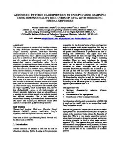
7. EXPERIMENTAL RESULTS 7.1 Maximizing information and clusters precision A first natural question to ask is what are the performance of the new sIB algorithm versus the AIB algorithm in terms of maximizing I(T ; Y ). Comparing the results over the 9 small data sets (for which running AIB is feasible) we found that sIB (with n=15) always extract solutions that preserve significantly more information than AIB (the improvement is of 17% on the average). Moreover, even if we do not choose for sIB the iteration which maximized I(T ; Y ) but compare all the 15 random restarts (for every data set) with the AIB results, we found that more than 90% of these runs preserve more information than AIB. The next question we address is whether clustering solutions that preserve more information are better correlated with the real statistical sources (i.e., the categories). In Figure 2(a) we present the progress of the information and precision for a specific restart of sIB over the NG10 data set. We clearly see that while the information is increasing for every assignment update (as guaranteed by the algorithm), P (T ) is increasing in parallel. In fact, less than 5% of the updates reduced P (T ). Similar results obtained for all the other data sets. 3

The underlying assumption here is that if the cluster is relatively homogeneous the user will be able to correctly identify its most dominant topic.

Information−Precision correlation for Multi5 tests

Information−Precision correlation for a specific restart

Information−Precision correlation for NG20

1 0.8

I(T;Y) P(T)

0.6 0.59

0.95

0.58 0.9

0.6

0.4

P(T)

P(T)

0.57 0.85 0.8

0.56 0.55 0.54

0.75 0.2

Multi5 1 Multi52 Multi53

0.7 0 0

0.5

1

1.5

2

2.5 4 x 10

0.65 0.57

0.58

0.59

(a)

0.6 I(T;Y)

(b)

0.61

0.62

0.63

0.53 0.52 0.51 0.74

0.745

0.75

0.755 I(T;Y)

0.76

0.765

(c)

Figure 2: (a) Progress of I(T ; Y ) and P (T ) during the assignment updates of sIB over the NG10 data set. Correlation of final values of I(T ; Y ) and P (T ) for all random restarts of sIB over (b) the three M ulti5 tests and (c) the NG20 test. Lastly, we would like to check whether choosing the iteration which maximized I(T ; Y ) is a reasonable unsupervised criterion for identifying solutions with high precision. In Figure 2(b,c) we see the final values of I(T ; Y ) versus P (T ) for all the n random restarts of sIB over the three M ulti5 tests and the NG20 test. Clearly these final values are correlated. In fact, in 9 out of our 13 tests the iteration which maximized I(T ; Y ) also maximized P (T ), and when it did not the gap was relatively small.

7.2 Results for small-scale experiments In Table 1 we present the results for the small-scale 9 subsets of the 20Newsgroups corpus. The results for the IDC algorithm are taken from [4]. For all the unsupervised algorithms we set n = 15, ε = 0 and maxL = 30. However, all algorithms except for sL1 attained full convergence in all 15 restarts and over all datasets after less than 30 loops. To gain some perspective about how hard is the classification task we also present results of a supervised Naive Bayes (NB) classifier (see [15] for the details of the implementation). The test set for this classifier consisted of the same 500 documents in each data set while the training set consisted of different 500 documents randomly chosen from the appropriate categories. We repeated this process 10 times and averaged the results. Several results should be noted specifically. • sIB outperformed all the other unsupervised techniques in all data sets, typically with an impressive gap. Taking into account that for the other techniques we present an “unfair” choice of the best result (among all 15 restarts) we see these results as especially encouraging. • In particular sIB was clearly superior to IDC and AIB which are both also motivated by the Information Bottleneck method. Nonetheless, in contrast to sIB, the specific implementation of IDC in [4] is not guaranteed to maximize I(T ; Y ) which might explain its inferior performance. We believe that the same explanation holds for the inferiority of AIB. • sIB was also competitive with the supervised NB clas-

sifier. A significant difference between these two was evident only for the three Multi10 subsets, i.e., only when the number of real categories was relatively high. • The poor performance of the sKL algorithm was due to a typical fast convergence into one huge cluster which consisted of almost all documents. This tendency is due to the over sensitivity of this algorithms to “zero” probabilities in the centroid representations and it was clearly less dominant in the medium scale experiments. • The AIB results are significantly better than those reported in [14] (P(T)=45.8) although the algorithm is the same. The difference is probably due to the inclusion of the subject lines of the messages, in contrast to these previous results.

7.3 Results for medium-scale experiments In Table 2 we present the results for the medium-scale data sets. To the best of our knowledge our results are the first reported results (using direct evaluation measures as precision and recall) for unsupervised methods over corpora in that scale (order of 104 documents). For all the unsupervised algorithms we set n = 10, ε = 10−2 |X| (where |X| is the number of documents in the corpus) and maxL = 10. We note here that this last choice of maxL = 10 was in fact probably too low for some of the algorithms (see below). For these tests as well we applied the supervised NB classifier. For each test, the training set consisted of 1, 000 documents, randomly chosen out of the dataset, while the test set consisted of the remaining documents. Again, we repeated this process 10 times and averaged the results. Notice that the two Reuters tests are multi-labeled while all our classification schemes are uni-labeled. Therefore the recall of these schemes is inherently limited. This is especially evident for the new-Reuters test in which the average number of labels per document was 1.78 and hence the maximum attained (micro-averaged) recall was limited to 56%. Our main findings are listed in the following. • Similar to the small-scale experiments, sIB outperforms all the other unsupervised techniques, typically

Table 1: Micro-averaged precision results over the small data sets. In all unsupervised algorithms the number of clusters was taken to be identical with the number of real categories (indicated in parenthesis). For Kmeans,sK-means,sL1 and sKL the results are the best results among all 15 restarts. For sIB the results are for the restart which maximized I(T ; Y );. The test set for the NB classifier consisted of the same 500 documents in each data set while the training set consisted of different 500 documents randomly chosen from the appropriate categories. We repeated this process 10 times and averaged the results. P (T ) Binary1 (2) Binary2 (2) Binary3 (2) M ulti51 (5) M ulti52 (5) M ulti53 (5) M ulti101 (10) M ulti102 (10) M ulti103 (10) Average

sIB 91.4 89.2 93.0 89.4 91.2 94.2 70.2 63.8 67.0 83.3

IDC 85 83 80 86 88 86 56 49 55 74.0

sK-means 62.4 54.6 63.2 47.0 47.0 57.0 31.0 32.8 33.8 47.6

K-means 65.6 61.8 64.0 47.4 46.0 50.4 30.8 31.0 31.4 47.6

AIB 84.0 59.8 85.0 56.6 63.8 76.8 42.4 34.0 38.8 60.1

sL1 74.4 58.0 76.6 51.6 45.2 52.4 34.2 31.2 31.4 50.6

sKL 50.4 50.2 51.8 20.6 20.6 20.6 10.4 10.0 10.2 27.2

NB 87.8 85.4 88.1 92.8 92.6 93.2 73.5 74.6 74.6 84.7

Table 2: Micro-averaged precision results over the medium scale data sets. In all the unsupervised algorithms the number of clusters was taken to be identical with the number of real categories (indicated in parenthesis). The NB classifier was trained over 1, 000 randomly chosen documents and tested over the remaining. We repeated this process 10 times and averaged the results. P (T ) NG10 (10) NG20 (20) Reuters (10) new-Reuters (10) Average

sIB 79.5 57.5 85.8 83.5 76.6

sK-means 76.3 54.1 64.9 66.9 65.6

with a significant margin and in spite of the “unfair” comparison. • Interestingly, sIB was almost competitive with the supervised NB classifier which was trained over 1, 000 labeled documents. • Both our sequential and parallel K-means implementations performed surprisingly well, especially over the uni-labeled NG10 and NG20 tests. As in the small data sets, the differences between the parallel and the sequential implementation were minor. • The convergence rate of the sIB and the sK-means algorithms were typically better than those of the other algorithms. In particular, sIB and sK-means converged in most of their iterations while, for example, sL1 did not converged in any iteration.

7.4 Improving clusters precision In supervised text classification one is able to trade precision versus recall by defining some thresholding strategy. In the following we suggest a similar idea for the unsupervised classification scenario. Notice that once a partition T is obtained we are able to estimate d(x, t(x)) ∀x ∈ X. Clearly this provide us with an estimate of how “typical” is x in t(x). Specifically in the context of sIB, d(x, t(x)) is related to the loss of information by not holding x as a singleton

K-means 70.3 53.4 66.4 67.3 64.4

sL1 27.7 15.3 70.1 73.0 46.5

sKL 58.8 28.8 59.4 81.0 57.0

NB 80.8 65.0 90.8 85.8 80.6

cluster. By sorting the documents in each cluster t ∈ T with respect to d(x, t) and “labeling” only the top r% of the documents in that cluster we can now reduce the recall while (hopefully) improving the precision. More specifically while defining the “label” for every cluster we use only documents that were sorted among the top r% for that cluster (and refer to the remaining as “unlabeled”). Notice that this procedure is independent of the specific definition of d(x, t) and thus could be applied for all the sequential algorithms we tested. In Figure 3 we present the Precision-Recall curves for some of our medium scale tests. Again, we find sIB to be clearly superior to all the other unsupervised methods examined. In particular for r = 10% sIB attains very high precision in a totally unsupervised manner for our real world corpora. These results raise the possibility of a new approach for combining unsupervised and supervised classification methods. Specifically we could use these high precision “labeled” clusters as a training set for a supervised classifier. Assuming that the precision of our “labels” is indeed relatively high and that the supervised classifier is not too sensitive for a small amount of “noise” in its training set, we predict that we can now label the remaining “unlabeled” documents (and new ones) with a reasonable performance. This issue, however, is left for future research.

Precision−Recall curve for NG10 test

Precision−Recall curve for Reuters test

Precision−Recall curve for new−Reuters test

0.9 0.9

0.95 0.8

0.9

0.7

P(T)

P(T)

P(T)

0.6

0.8

0.75

0.5 sIB sL1 sKL sK−means

0.4 0.3 0

0.85

0.85

0.2

0.4 R(T)

0.6

0.8

sIB sL1 sKL sK−means

0.7 0.65 0.6 0

0.2

0.4 R(T)

0.6

0.8

0.75

sIB sL1 sKL sK−means

0.7

0.8

0

0.1

0.2

0.3

0.4

R(T)

Figure 3: Precision-Recall curves for some of our medium scale tests. For the other tests the results were similar. Notice that the results for sIB are for the specific restart which maximized I(T ; Y ) while for the other methods we present the best result over all 10 restarts.

7.5 Using other representations

8. CONCLUDING REMARKS

It is well known that a word-counts representation of documents is typically noisy and different techniques can provide more sophisticated representations. In this work we concentrated on comparing different algorithms for a fixed (counts) representation. Nonetheless, it is interesting to ask what are the performance using different representations. Although this is not the focus of this work we performed additional experiments regarding this issue. A well known approach in the context of text classification is the tf-idf representation [11]. Specifically, each word count is multiplied by the inverse-document-frequency of the word, defined by |X| idf (y) = log( |X(y)| ) where |X(y)| is the number of documents in which y occurred. Rich empirical evidence support the benefits of using this representation for text processing applications. Therefore we applied the sK-means and the parallel Kmeans for all our tests, using the tf-idf representation. The results presented in Table 3 indeed verify that this representation could significantly improve K-means performance. The improvement is especially impressive for the small (and more noisy) data sets and for the multi-labeled Reuters data sets. Interestingly, under this representation we see that the sequential implementation yield superior performance to the parallel one, which implies better robustness to local optima using a sequential approach. Comparing sIB with these results we still see that sIB attained superior performance in almost all our tests (although the gap in some cases was minor). Recall that this comparison is with the best result obtained using the tf-idf representation over all n restarts. Comparing sIB with the averaged tf-idf performance we obviously see a more significant margin in favor of sIB. These results are of special interest taking into account that the tf-idf representation is specifically “tailored” for the context of text classification while sIB is a general approach using the naive counts representation. Moreover, there is strong empirical evidence suggesting that sIB might improve its performance using more robust representations such as word-clusters [4, 14, 16].

In this paper we introduced the sIB algorithm. We showed that it has several important advantages over the agglomerative IB algorithm, both in terms of complexity and quality of clusters it finds. The reduced complexity allows us to use this algorithm on larger datasets. Moreover, the performance of sIB are superior to all the other unsupervised methods we examined, including methods which are especially designed for text classification. Additionally, our unsupervised results are even competitive with a standard supervised Naive Bayes classifier. In the appendix below, we provide preliminary theoretical analysis to motivate these empirical observations. An interesting question is comparing sIB with the parallel versions of IB algorithms [17]. Our preliminary results showed, rather surprisingly, that using sIB we seem to obtain solutions that preserve more information than by solving the self-consistent equations directly. However, this issue calls for a more thorough investigation and theoretical understanding. Lastly, we note here that extending the sIB algorithm to solve multi-variate variations of the Information Bottleneck principle [6] is straightforward, using the recent extension of the AIB algorithm into the multi-variate case [16].

Acknowledgments We thank Yoram Singer, Leo Kontorovich, Benjy Weinberger, and in particular Koby Crammer for useful discussions and comments on previous drafts of this paper. This work was supported in part by the Israel Science Foundation (ISF) and by the US-Israel Bi-national Science Foundation (BSF). N. Friedman was also supported by an Alon fellowship and the Harry & Abe Sherman Senior Lectureship in Computer Science.

9. REFERENCES

[1] R. Bekkerman, R. El-Yaniv, Y. Winter, and N. Tishby. On Feature Distributional Clustering for Text Categorization. In ACM SIGIR 2001, 2001. [2] T. M. Cover and J. A. Thomas. Elements of Information Theory. John Wiley & Sons, New York, 1991.

Table 3: Micro-averaged precision results using tf-idf representation. The first row present the average performance over the small 9 tests. The results for sIB, sK-means and K-means are repeated for convenience. For all algorithms except for sIB we present the best result among all restarts. For the tf-idf representation we also present in parenthesis the averaged results over all restarts. P (T ) Small 10NG 20NG Reuters new − Reuters Average

sIB 83.3 79.5 57.5 85.8 83.5 77.9

sK-means 47.6 76.3 54.1 64.9 66.9 62.0

tf-idf:sK-means 81.4 (67.7) 76.1 (70.8) 58.4 (54.9) 85.4 (81.8) 81.5 (77.7) 76.6 (70.6)

[3] K. Eguchi. Adaptive Cluster-based Browsing Using Incrementally Expanded Queries and Its Effects. In ACM SIGIR 99, 1999. [4] R. El-Yaniv and O. Souroujon. Iterative Double Clustering for Unsupervised and Semi-supervised Learning. In Proc. of Neural Information Processing Systems (NIPS-14), 2002, to appear. [5] M. A. Hearst and J. O. Pedersen. Reexamining the Cluster Hypothesis: Scatter/Gather on Retrieval Results. In ACM SIGIR 96, 1996. [6] N. Friedman, O. Mosenzon, N. Slonim, and N. Tishby. Multivariate Information Bottleneck. In Proc. of the 17th conf. on Uncertainty in artificial Intelligence (UAI-17), 2001. [7] K. Lang. Learning to filter netnews. In Proc. of the 12th Int. Conf. on Machine Learning, 1995. [8] J. Lin. Divergence Measures Based on the Shannon Entropy. IEEE Transactions on Information theory, 37(1), 1991. [9] R. M. Neal and G. E. Hinton. A view of the EM algorithm that justifies incremental, sparse, and other variants. In M. I. Jordan (editor), Learning in Graphical Models, pp. 355-368, 1998. [10] F. C. Pereira, N. Tishby, and L. Lee. Distributional clustering of English words. In 30th Annual Meeting of the Association for Computational Linguistics, Columbus, Ohio, 1993. [11] G. Salton. Developments in Automatic Text Retrieval. Science, Vol. 253, pages 974–980, 1990. [12] A. Schriebman, R. El-Yaniv, S. Fine and N. Tishby. On the two-sample problem and the Jensen-Shannon divergence for Markov sources. In preparation. [13] N. Slonim and N. Tishby. Agglomerative Information Bottleneck. In Proc. of Neural Information Processing Systems (NIPS-12), 1999. [14] N. Slonim and N. Tishby. Document Clustering using Word Clusters via the Information Bottleneck Method. In ACM SIGIR 2000, 2000. [15] N. Slonim and N. Tishby. The power of word clusters for text classification. In 23rd European Colloquium on Information Retrieval Research (ECIR), 2001. [16] N. Slonim, N. Friedman and N. Tishby. Multivariate Agglomerative Information Bottleneck. In Proc. of Neural Information Processing Systems (NIPS-14), 2002, to appear. [17] N. Tishby, F. Pereira, and W. Bialek. The Information

K-means 47.6 70.3 53.4 66.4 67.3 61.0

tf-idf:K-means 61.9 (51.3) 71.9 (67.8) 54.1 (51.6) 82.8 (76.6) 79.5 (77.7) 70.0 (65.0)

Bottleneck method. In Proc. 37th Allerton Conference on Communication and Computation. 1999. [18] C. J. van Rijsbergen. Information Retrieval. London: Butterworths; 1979. [19] O. Zamir and O. Etzioni. Web Document Clustering: A Feasibility Demonstration. In ACM SIGIR 98, 1998.

APPENDIX A.

CLUSTERS ACCURACY AND MUTUAL INFORMATION

In the following we give some preliminary theoretical analysis which relates information maximization clustering with supervised classification. We assume the following setting. We are given a set of objects x ∈ X which are represented as conditional distributions p(y|x). The true (unknown) classification of these objects induces a partition of X into K disjoint classes where each class is characterized through a distribution p(y|ck ), ck ∈ C . Denoting the class of some specific x ∈ X by c(x) we assume the following (strong) asymptotic assumption: p(y|x) = p(y|c(x)) ∀x ∈ X. In the context of document classification p(y|x) is typically the relative frequencies of the words y ∈ Y in some document x while p(y|c(x)) represent the relative frequencies of the words over all the documents that belong to the class c(x). Therefore, the violation of this assumption becomes less severe as the sample size for p(y|x) (i.e., the length of the document x) is increased. Using the labeling scheme described in section 6.2, for any given partition the micro-averaged precision P (T ) is well defined. In particular, if we denote by T ∗ the partition which is perfectly correlated with the true classes, then clearly P (T ∗ ) = 1. Notice that every partition T defines a set of “hard” membership probabilities p(t|x). These probabilities in turn, defines through Eqs.(3) (using the Markov independence assumption between T and Y given X) the set of centroid distributions p(y|t) and prior distribution p(t). Therefore, for any partition T , I(T ; Y ) is well defined. Under the above assumption we get: Proposition A.1. I(T ∗ ; Y ) > I(T ; Y ) for any partition T 6= T ∗ such that |T | = K. Thus, the “true” partition T ∗ , maximizes the information, and by definition the precision. Nonetheless, this proposition refers only to the perfect partition and does not provide insight about the information preserved by other partitions. We define the distortion of some partition T with respect to the true classification by D(T ) ≡ EP (x) [DKL (P (Y | c(x))||P (Y | t(x)))]. Based on our asymptotic assumption, we then get: Proposition A.2. D(T (1) ) ≤ D(T (2) ) ⇐⇒ I(T (1) ; Y ) ≥ I(T (2) ; Y ) Hence, roughly speaking, seeking partitions which are more similar to the true classification is equivalent to seeking partitions that are more informative about the feature space Y .