cesses for mining these data become highly ex- pensive ... gorithms, such as iterative refinement (Zhao and .... the previous one with a different bias, a different.
Unsupervised Document Clustering by Weighted Combination Edgar Gonz`alez and Jordi Turmo TALP Research Center {egonzalez,turmo}@lsi.upc.edu Abstract This report proposes a novel unsupervised document clustering approach based on weighted combination of individual clusterings. Two non-weighted combination methods are adapted to work in a weighted fashion: a graph based method and a probability based one. The performance of the weighted approach is evaluated on realworld collections, and compared to that of individual clustering and non-weighted combination. The results of this evaluation confirm that graph based weighted combination consistently outperforms the other approaches.
1 Introduction As the availability of large amounts of textual information is unlimited in practice, supervised processes for mining these data become highly expensive for human experts. For this reason, unsupervised methods are being a central topic for researchers on tasks related to text mining. One of these tasks is unsupervised document clustering, which is the focus of this report. Unsupervised document clustering can be defined as the process of grouping similar documents without knowing a priori the number of document categories. Classical methods used for this task are based on two steps: clustering candidate generation and best candidate selection. In the first step, a set of clusterings πj is generated, each one consisting of a different number kj of groups of documents or clusters. Hierarchical algorithms generate the set of clusterings by building a tree representation of the clusters, or dendrogram, without supervision (Hatzivassiloglou et al., 2000). Other approaches are based on the use of supervised clustering algorithms, such as iterative refinement (Zhao and Karypis, 2004) or matrix factorization (Xu et al., 2003) among others. These approaches repeatedly apply the supervised clustering algorithm for an increasing number of clusters kj . In the second step, the best clustering is selected by means of a
criterion function (Calinski and Harabasz, 1974; Rissanen, 1978). Other unsupervised methods use a hybrid strategy in which a supervised clustering method is used to improve an initial solution found by means of an unsupervised method (Surdeanu et al., 2005). However, each one of these methods has an intrinsic and particular bias, uses a certain document representation, and depends on a document similarity measure. All these assumptions guide the clustering process, and lead it to a particular solution that may not be the optimal clustering. To overcome this limitation, recent research has focused on clustering combination. From a general point of view, the problem of clustering combination can be defined as: Given multiple clusterings of the data set, find a combined clustering with better quality (Topchy et al., 2005). The most popular methods in the state of the art are graph partitioning based (Strehl and Ghosh, 2002) and probability based (Topchy et al., 2005). Probability based clustering combination has already been applied to document collections, as in (Topchy et al., 2005), based on expectation-maximization (EM), and in (Siersdorfer and Sizov, 2004), based on voting following a probabilistic model. These combination approaches give the same relevance to each individual clustering. However, different clustering methods may be more or less suitable for different data collections, according to how the collections accomplish the assumptions of the method. It is hence sensible to think of a weighted combination of clusterings, in which better clusterings contribute more to the final result. This makes necessary to find a strategy to determine the weights of each clustering in the combination. This report presents a generic approach for unsupervised document clustering, based on the automatic selection of the best weighted combination of individual clusterings for a given document collection. We compare a graph based method and a probability based one to perform weighted and non-weighted combination of individual clusterings, evaluate their performance in different col-
{wj }
Individual Clustering Individual Clustering
k 1
Clustering
1
k
2
Clustering
2
... Document Collection
Individual Clustering
{wj }
{wj }
k
r
Clustering
r
{wj }
k
Clustering Combination
Clustering
1
Clustering Combination
Clustering
2
Clustering Selection
Clustering Combination ...
Clustering
3
Clustering Combination
Clustering
s
Output Clustering
Figure 1: The weighted clustering approach
lections, and show that graph based weighted combination outperforms individual clustering, as well as the other tested combination methods. The rest of the report is organized as follows: Section 2 introduces this generic approach. Sections 3 and 4 detail the individual clustering algorithms and the combination methods used in the experiments, respectively. Section 5 describes the experiments carried out and gives a summary of their results. Finally, Section 6 concludes this report.
2 Generic Approach The proposed approach is depicted in Figure 1, and proceeds in three steps: 1. Generate the initial clusterings, {π j }, each one with number of clusters kj , applying different individual unsupervised clustering methods, {Ij }, to the input document collection. 2. Generate weighted combination clusterings, π ¯α , from the initial ones, {πj }, using the clustering combination method with different sets of weights, {wj }α , and numbers of clusters, k¯α . Following the usual cluster ensemble problem statement (Strehl and Ghosh, 2002), the combination method does not access the document representation used by the individual clustering methods. 3. Select the best weighted combination clustering π ¯ from those generated in step 2. This approach defines a family of weighted combination methods. Sections 3 and 4 describe different choices of components for the three steps.
3 Unsupervised Individual Clustering As mentioned before, the particular bias of the individual clustering methods, as well as the type
of document representation and similarity measure they use, imply a different point of view of the documents. In order to carry out our experiments, we have used a heterogeneous set of unsupervised individual clustering methods. The first one of them is a geometric hybrid method (Surdeanu et al., 2005), which has been shown to give good performance for unsupervised document clustering of different real-world collections. The second one is an informationtheoretical hybrid method, which is a version of the previous one with a different bias, a different document representation and a different similarity measure. And the third one is a classical method consisting of a hierarchical algorithm and a criterion function to determine the best clustering. A description of each one of them follows. 3.1
Geometric Hybrid Method
An outline of the method presented in (Surdeanu et al., 2005) is shown in Figure 2, and is described below: The process starts finding a good initial clustering for an iterative refinement algorithm. This kind of algorithm requires the number of clusters to be provided, and is sensitive to this choice. This is why a good estimation of the number of clusters is mandatory for a good initial clustering, even if some documents remain uncovered. The initial clustering is found by applying a classical method: 1. A hierarchical algorithm is used to find a dendrogram. 2. A set of initial clustering candidates is generated for different degrees of document coverage and different cluster quality measures. Each one of the candidates consists of the list of the best clusters from the whole set present in the dendrogram, ranked taking into account a specific degree of document cover-
Hierarchical Clustering
Select Best Initial Model
Generate Initial Model Candidates
Iterative Clustering
Figure 2: The hybrid clustering method age and a specific cluster quality measure 1 . This implies that some documents may not occur in any cluster of the list. 3. The best clustering candidate is selected by applying a global quality measure. In (Surdeanu et al., 2005), the method is specified using a geometric point of view: • Documents are represented as tf · idf vectors of words. • The distance between two documents is computed by the cosine distance. • The hierarchical algorithm used is Hierarchical agglomerative clustering (HAC). • The global quality function is computed by Calinski and Harabasz’s C score (Calinski and Harabasz, 1974). • The iterative refinement algorithm applied is EM. We will refer henceforth to this method as Geo. 3.2
theory that could be useful to define a document distance, such as Kullback-Leibler divergence or mutual information. However, on the contrary of Jensen-Shannon divergence, they are not symmetric or require absolute continuity. • The hierarchical algorithm used is agglomerative information bottleneck method (aIB) (Slonim, 2003). • The global quality function is computed as the length of the message encoding the documents in the clustering candidate, as described below. Classical informationtheoretical selection criteria, such as minimum description length or minimum message length, require a probability distribution, which cannot be inferred from the dendrogram. • The iterative refinement algorithm applied is divisive information-theoretical clustering (DITC) (Dhillon and Guan, 2003). The length of the message encoding each clustering candidate, π, is computed as:
Information-Theoretical Hybrid Method
Recently, there has been an interest in applying information theoretical measures to the task of document clustering (Dhillon and Guan, 2003; Slonim, 2003). For this reason, and to find a view of the data different from Geo, we have adapted the aforementioned hybrid method to use informationtheoretical measures, as follows: • Documents are represented as probability distributions of words. • The distance between two documents is computed by Jensen-Shannon divergence. There are other measures coming from information
Length(π) =
LM C + L C + L D kdl | dl ∈ πk
where • LM C is the length of encoding the metacentroid mc of the clustering using a code fixed a priori. • LC is the length of encoding the centroid c i of each cluster C i using a code based on the frequency of words in the meta-centroid mc. LC = −
XX Ci
p(w|ci ) · log p(w|mc)
w
1
For simplicity, the set of cluster quality measures has been elided in this report. For more details, see (Surdeanu et al., 2005)
• LD is the length of encoding each document dl using a code based on the frequency of
words in the centroid ci of its cluster C i . LD = −
X X X Ci
dl
∈C i
p(w|dl ) · log p(w|ci )
w
• kk stands for the cardinality of a set. This formula was the one to give the best results in preliminary experiments, compared against a version of Calinski and Harabasz’s score using Jensen-Shannon divergence. We will refer to this method as IT. 3.3
Hierarchical Method
The third clustering method is a classical method based on a hierarchical algorithm. A dendrogram is built using the aIB algorithm, and Calinski and Harabasz’s C score is used to find the level of the dendrogram at which the best clustering occurs. We will refer to it as HiIT.
4 Weighted Combination We have adapted two non-weighted clustering combination methods to deal with a weighting of the initial clusterings. The first one (Strehl and Ghosh, 2002) is based on solving graph partition problems, whereas the second one (Topchy et al., 2005) is based on using EM. To describe these methods, we will use a formalization of clustering combination. Having D = {d1 . . . dn } a set of documents, a clustering πj of this set is a partition of D into a set k {Cj1 . . . Cj j } of kj disjoint clusters Cji . Each cluster Cji can be identified by its numerical label i. The clustering πj can also be viewed as a function mapping documents into labels: πj : D → {1 · · · kj }
(1)
The aim of clustering combination is to find a clustering π ¯ , of k¯ clusters, which is the consensus of r clusterings {πj } = {π1 . . . πr }, by means of a consensus function Γ. If we consider a weighted combination of clusterings, for each initial clustering πj a weight wj is defined. 4.1
Graph based Method
(Strehl and Ghosh, 2002) proposes several methods to combine a cluster ensemble and produce a single output clustering, based on solving graph partition problems. In addition, it offers a criterion to select which method to use in each case, using a normalized mutual information measure.
Given initial clusterings {πj }, and the number ¯ three graph partition probof desired clusters k, lems are solved to obtain three possible combinations π ¯: CSPA (Cluster based Similarity Partitioning Algorithm) A graph is built in which every document da ∈ D is a vertex. The weight of the edge between da and db is the number of clusterings πj in which the documents lie in the same cluster, kπj | πj (da ) = πj (db )k. A partition of this graph into k¯ clusters is found, and the combination is the induced clustering on D. HGPA (HyperGraph Partitioning Algorithm) A hypergraph is built in which every document d a ∈ D is a vertex. Each cluster Cji in each initial clustering πj is a hyperedge, and the hypergraph is partitioned into k¯ clusters. The combination is the induced clustering on D. MCLA (Meta-CLustering Algorithm) A graph is built in which every cluster Cji in each initial clustering πj is a vertex. The weight of an edge be0 tween clusters Cji and Cji0 is the Jaccard measure 0 0 of the two sets: |Cji ∩ Cji0 |/|Cji ∪ Cji0 |. This graph is partitioned into k¯ so-called meta-clusters γq . In the combination, each document dl is assigned to the meta-cluster to which it contributes the most, this is arg maxγq kCji ∈ γq | dl ∈ Cji k. To decide which of the three combinations π ¯ is the best, the measure of normalized mutual information (NMI) between two clusterings is defined as: N M I(πj , πj 0 ) = q
I(πj , πj 0 ) H(πj ) · H(πj 0 )
where I and H are the usual mutual information and entropy, respectively. For each one of the three obtained combinations π ¯ , the average normalized mutual information (ANMI) with respect to the initial clusterings {πj } is: AN M I(¯ π , {πj }) =
P
N M I(¯ π , πj ) kπj k
The obtained π ¯ with the highest ANMI is selected as the best combination. 4.1.1 Weighted Version To incorporate weighting into this method, the graphs produced by the three methods have been modified:
CSPA The weight of the edge between documents da and db is the sum of the weights of the clusterings πj in which the documents lie in the same P cluster, wj | πj (da ) = πj (db ).
¯
P (yl | Θ) =
HGPA The weight of the hyperedge representing cluster Cji is the weight wj of the clustering πj to which the cluster belongs. MCLA The weight of the edge between clusters 0 Cji and Cji0 is the Jaccard measure of the two sets, multiplied by the weights of the clusterings π j and 0 πp to which the clusters belong: |Cji ∩ Cji0 |/|Cji ∪ 0 Cji0 | · wj · wj 0 In all cases, the non-weighted version is equivalent to assign a weight of wj = 1 to all clusterings πj . The ANMI function has been turned to a weighted normalized mutual information (WNMI), in which the NMI of π ¯ with respect to each initial clustering πj is weighted by wj :
k X
αm P (yl | Θm ) (3)
m=1 r Y
P (yl | Θm ) =
P (ylj | Θmj )
(4)
ϑmjk δ(ylj ,k)
(5)
j=1 ¯
kj Y
P (ylj | Θmj ) =
k=1
where αm is the probability of each mixture a priori, ϑmjk is the probability of feature j in mixture m taking value k, and δ stands for the function evaluating to 1 if its arguments are equal and to 0 otherwise. The model parameters, Θ, are estimated using EM and the combination clustering π ¯ is obtained by assigning each document to the most probable mixture component: π ¯ (dl ) = arg max P (yl | Θm ) m
W N M I(¯ π , {πj }) =
P
wj · N M I(¯ π , πj ) P (2) wj
As in (Strehl and Ghosh, 2002), we have used the freely available2 packages M ETIS and HM ETIS to solve the graph and hypergraph partition problems.
4.2.1 Weighted Version The most natural weighted extension to the previous approach is to use weighted naive Bayes models. Equations 3 and 5 remain the same, and weights are introduced into Equation 4, as follows: P (yl | Θm ) =
r Y
0
P (ylj | θmj )wj
j=1
4.2
Probability based Method
(Topchy et al., 2005) introduces a probabilistic view of combination, which is solved using EM. Given initial clusterings {πj }, and the number ¯ a matrix Y can be defined of desired clusters k, with as many rows as documents in the clusterings, and as many columns as initial clusterings. Each entry ylj stands for the label of the cluster to which document dl belongs in clustering πj , as computed with Equation 1. These labels are random variables drawn from a probability distribution described as a mixture of k¯ multi-variate component densities. A document dl can be represented by its labels yl = (yl1 . . . ylr ). If the naive Bayes assumption is taken, with respect to the independence of the labels given the class, and each label ylj is seen as drawn from a multinomial distribution, the probability of yl is: 2 http://glaros.dtc.umn.edu/gkhome/ views/metis/
These weights wj0 must be normalized so they add up to the number of initial clusterings r. EM is also used to train this model. 4.3
Clustering Selection
The set of weighted combination clusterings {¯ πα } is virtually infinite. Selecting the best combination can be seen as a search problem. As an exhaustive search is highly expensive, we have pruned the search space of possible π ¯ α to those satisfying the following restrictions: k¯ ∈ {bmin kj − σk c . . . dmax kj + σk e} wj
∈ {1 . . . G}
where kj is the number of clusters in initial clustering πj , σk is the standard deviation of kj , and G is a parameter. The number k¯ of clusters that a combination clustering can contain is thus limited to values in
the interval defined by the minimum and maximum number of clusters found by the individual clustering methods, extended by the standard deviation σk in both directions. If there is good agreement between all individual methods, σ k will be small and the best k¯ will be close to the individual kj . On the contrary, if the individual k j differ considerably, σk will be large, and the best k¯ can be outside the interval of kj . Parameter G allows to prune the combinations by limiting the weights to natural values ranging from 1 to G. The larger the value of G, the finer the tuning of the weights. For our experiments, we have taken a value of G = 4. To select the best combination from all the possible weighted combination clusterings, π ¯ α, a scoring function η to be maximized is used: • For graph based combination, the score is weighted normalized mutual information, as defined in Equation 2. • For EM based combination, the score is the log-likelihood of the clustering given the probabilistic model found: LL(¯ π) =
X
where P is defined in Equation 3.
5 Experiments Evaluation Data
The collections used in our experiments are: APW The Associated Press (year 1999) subset of the AQUAINT collection. The document category assignment is indicated by a CATEGORY tag. LATIMES The Los Angeles Times subset of the TREC-5 collection. The categories correspond to the newspaper desk that generated the article (Zhao and Karypis, 2004). Reuters The by now classic Reuters-21578 text categorization collection. Similarly to previous work, we use the ModApte split (Nigam et al., 2000), but, since our algorithms are unsupervised, we use the test partition directly. Reuters10 A subset of the above ModApte test partition that includes only the ten most frequent categories. SMART A collection previously developed and used for the evaluation of the SMART information retrieval system.
kDk 5000 5000 3019 2545 5467
kΛk 11 8 93 10 4
Terms 27366 31960 7846 6734 11950
Table 1: Evaluation data sets Due to memory limitations on our test machines, the size of the APW and LATIMES collections is reduced to the first 5,000 documents (the complete collections contain over 100,000 documents). The documents are preprocessed by discarding stop words and numbers, converting all words to lower case, and removing terms occurring in a single document (Zhao and Karypis, 2004). Table 1 lists the collection characteristics after preprocessing: number of documents (kDk), categories (kΛk) and terms. In the two Reuters collections, the assignment of documents to categories is ambiguous: the mean number of categories assigned to a document is 1.2 in the Reuters collection and 1.1 in the Reuters10 collection. 5.2
logP (yl | Θ)
dl
5.1
Collection APW LATIMES Reuters Reuters10 SMART
Evaluation Measures
The quality of the clustering solutions is measured using the metrics of purity, inverse purity and F 1 . These metrics are widely used to evaluate the performance of unsupervised clustering algorithms (Zhao and Karypis, 2001). Purity (Pur) evaluates the degree to which each cluster contains documents from a single category λj . The purity of a cluster C i is the ratio of the cluster size, kC i k, that the largest category of documents assigned to C i represents. (Zhao and Karypis, 2004). The overall purity is the weighted average of all cluster purities: P ur(C i ) = P ur =
1 max kC i ∩ λj k kC i k j k X kC i k i=1
kDk
P ur(C i )
Inverse purity (IPur) evaluates the degree to which the documents in a category are grouped in a single cluster. The inverse purity of a category λj is the ratio of the category size, kλ j k, that the cluster with the largest number of documents in that category represents. The overall inverse purity is the weighted average of all category inverse purities:
IP ur(λj ) =
1 max kC i ∩ λj k kλj k i kΛk
IP ur =
X kλj k
j=1
kDk
IP (λj )
APW
LATIMES
Reuters
The F1 measure is the harmonic mean of purity and inverse purity: 2 · P ur · IP ur F1 = P ur + IP ur We also consider the number of clusters found, k, as an indicator of good solutions, although this factor is already considered inside the other measures: a bad estimation of k gives low values of either purity or inverse purity, and hence, of F 1 .
Reuters10
SMART
Results
We have compared the performance of the individual clustering methods as well as the weighted and non-weighted combination methods on the evaluation data collections. The results obtained by the individual clustering methods3 are listed in Table 2. The best method in terms of F1 is presented in bold face. The Geo method is the best in Reuters, Reuters10 and SMART collections, and usually gives the most balanced results (P ur ≈ IP ur). HiIT stands out in APW, but often underestimates k. This is why it performs well in terms of inverse purity, yet suffers from low purity. IT is the best in LATIMES, because although its F1 is the same as HiIT’s, its estimated k is better. Table 3 shows the results for the combination methods. It presents the results obtained by the graph based method (Gr) and the probability based method (EM). For both, we give the results obtained so by non-weighted combination (Eq) as by weighted combination, estimating the best weights using the procedure in Section 4.3 (W). The graph based weighted method is the one that achieves the best F1 in all collections but in APW, where EM.W is better. Moreover, in the other four collections the graph based combination methods perform better or equal than the individual clustering methods in all four considered measures. Regarding the difference between weighted and non-weighted versions of combination, Gr.W is 3
The results shown are those from our implementation of method Geo, although they slightly differ from those in (Surdeanu et al., 2005)
Pur 0.74 0.72 0.63 0.75 0.75 0.66 0.68 0.68 0.57 0.77 0.77 0.73 0.91 0.89 0.71
IPur 0.72 0.56 0.88 0.56 0.61 0.68 0.83 0.76 0.82 0.85 0.76 0.86 0.77 0.58 0.97
F1 0.73 0.63 0.74 0.64 0.67 0.67 0.75 0.71 0.67 0.81 0.76 0.79 0.83 0.71 0.82
k 10 8 3 14 7 6 8 7 4 6 6 4 6 9 3
Table 2: Results of the individual methods
APW
5.3
Method Geo IT HiIT Geo IT HiIT Geo IT HiIT Geo IT HiIT Geo IT HiIT
LATIMES
Reuters
Reuters10
SMART
Method Gr.Eq Gr.W EM.Eq EM.W Gr.Eq Gr.W EM.Eq EM.W Gr.Eq Gr.W EM.Eq EM.W Gr.Eq Gr.W EM.Eq EM.W Gr.Eq Gr.W EM.Eq EM.W
wj 2+1+3 1+1+4 1+3+1 1+4+1 3+3+4 1+1+4 4+3+4 1+1+4 1+3+3 1+1+4
Pur 0.71 0.72 0.73 0.63 0.75 0.76 0.78 0.75 0.70 0.71 0.72 0.57 0.81 0.82 0.82 0.73 0.91 0.92 0.91 0.71
IPur 0.73 0.72 0.64 0.88 0.68 0.68 0.53 0.61 0.86 0.86 0.71 0.82 0.84 0.85 0.82 0.86 0.91 0.91 0.68 0.97
F1 0.72 0.72 0.68 0.74 0.72 0.72 0.63 0.67 0.77 0.78 0.71 0.67 0.83 0.83 0.82 0.79 0.91 0.92 0.78 0.82
k 7 7 11 3 7 8 16 7 7 9 10 4 7 7 8 4 4 5 11 3
Table 3: Results of the combination methods better than Gr.Eq in all cases. Only in the determination of k in the SMART collection the latter works better than the former (k = 5 for Gr.W, while k = 4 = kΛk for Gr.Eq). Although the differences between Gr.Eq and Gr.W are small, we believe that the addition of weighting represents an improvement, specially because the weights are found automatically. On the contrary, the results obtained by the probability based methods EM are not so satisfactory. In all but the APW collection, the results are lower than using the graph based ones Gr, and also lower than the results obtained by some individual methods (e.g., Geo and IT in the Reuters collection). For the EM methods the results are variable and it cannot be concluded that the weighted combination strategy outperforms its individual components, as occurs with Gr methods.
We think that a possible explanation for the behavior of the EM methods lies in the nature of the log-likelihood function that is used to determine the weights. It is biased towards solutions with lower k. For this reason, EM.W selects combinations where a single initial clustering has most of the weight with the lowest possible number of clusters. For instance, for the APW collection, the combination assigns the maximum weight to HiIT, which achieves the lowest value of k = 3. The same behavior can be seen in the rest of collections, with the exception of LATIMES. We think this exception may be explained by IT and HiIT solutions being very similar.
istry of Universities, Research and Information Society (DURSI) of the Catalan Government, and the European Social Fund. Our research group, TALP Research Center, is recognized as a Quality Research Group (2001 SGR 00254) by DURSI.
6 Conclusions
V. Hatzivassiloglou, L. Gravano, and A. Maganti. 2000. An investigation of linguistic features and clustering algorithms for topical document clustering. In Proceedings of SIGIR’00, pages 224–231.
This report presents a novel approach for unsupervised document clustering based on weighted combination of individual clusterings. Briefly, our approach is three-fold: first, a set of initial clusterings are induced using different individual clustering methods; second, all possible weighted combinations of these initial clusterings are performed using different numbers of clusters and sets of weights; third, the best weighted combination is selected. This approach has advantages over both individual clusterings and non-weighted combinations. First, it takes into account all the points of view considered by each individual clustering method. Second, weighted combinations can provide better solutions than non-weighted ones, given that for different document collections, the point of view of some individual clusterings can be more relevant than those of others. We have carried out a set of experiments with five real-world document collections. In these experiments, we have considered three heterogeneous individual clustering methods and two different weighted clustering combination methods. Bearing in mind the results of our experiments, we believe that weighted combination methods are better than the other methods considered. The most promising option seems to be a graph based weighted combination, which consistently gives the best results across all the data collections tested.
Acknowledgements This work has been supported by the European Comission (CHIL, IST-2004-506909), the Min-
References T. Calinski and J. Harabasz. 1974. A dendrite method for cluster analysis. Communications in Statistics, 3:1–27. I.S. Dhillon and Y. Guan. 2003. Information theoretic clustering of sparse co-occurrence data. In Proceedings of IEEE International Conference on Data Mining.
K. Nigam, A. McCallum, S. Thrun, and T. Mitchell. 2000. Text classification from labeled and unlabeled documents using em. Machine Learning, 39(2/3). J.J. Rissanen. 1978. Modelling by shortest data description. Automatica, 14:465–471. S. Siersdorfer and S. Sizov. 2004. Restrictive clustering and metaclustering for self-organizing document collections. In Proceedings of the SIGIR’04, pages 226–233. N. Slonim. 2003. The Information Bottleneck: Theory and Applications. Ph.D. thesis, The Hebrew University. A. Strehl and J. Ghosh. 2002. Cluster ensembles - a knowledge reuse framework for combining multiple partitions. Journal of Machine Learning Research, 3:583–617. M. Surdeanu, J. Turmo, and A. Ageno. 2005. A hybrid unsupervised approach for document clustering. In Proceedings of the KDD’05. A. Topchy, A.K. Jain, and W. Punch. 2005. Clustering ensembles: Models of consensus and weak partitions. IEEE Transactions on Pattern Analysis and Machine Intelligence, 27(12). W. Xu, X. Liu, and Y. Gong. 2003. Document clustering based on non-negative matrix factorization. In Proceedings of the ACM SIGIR’03. Y. Zhao and G. Karypis. 2001. Criterion functions for document clustering - experiments and analysis. Technical report, University of Minnesota, Department of Computer Science / Army HPC Research Center. Y. Zhao and G. Karypis. 2004. Empirical and theoretical comparisons of selected criterion functions for document clustering. Machine Learning, 55(3).