Hindawi Publishing Corporation Advances in Materials Science and Engineering Volume 2013, Article ID 196382, 9 pages http://dx.doi.org/10.1155/2013/196382
Research Article Upset Prediction in Friction Welding Using Radial Basis Function Neural Network Wei Liu,1,2 Feifan Wang,3 Xiawei Yang,3 and Wenya Li3,4 1
State Key Laboratory of Integrated Service Networks, Xidian University, Xi’an, Shaanxi 710071, China Department of Physics, Qinghai Normal University, Xining, Qinghai 810008, China 3 State Key Laboratory of Solidification Processing, Northwestern Polytechnical University, Xi’an, Shaanxi 710072, China 4 School of Materials Science and Engineering, Northwestern Polytechnical University, Xi’an, Shaanxi 710072, China 2
Correspondence should be addressed to Wenya Li;
[email protected] Received 18 August 2013; Accepted 9 October 2013 Academic Editor: Achilleas Vairis Copyright © 2013 Wei Liu et al. This is an open access article distributed under the Creative Commons Attribution License, which permits unrestricted use, distribution, and reproduction in any medium, provided the original work is properly cited. This paper addresses the upset prediction problem of friction welded joints. Based on finite element simulations of inertia friction welding (IFW), a radial basis function (RBF) neural network was developed initially to predict the final upset for a number of welding parameters. The predicted joint upset by the RBF neural network was compared to validated finite element simulations, producing an error of less than 8.16% which is reasonable. Furthermore, the effects of initial rotational speed and axial pressure on the upset were investigated in relation to energy conversion with the RBF neural network. The developed RBF neural network was also applied to linear friction welding (LFW) and continuous drive friction welding (CDFW). The correlation coefficients of RBF prediction for LFW and CDFW were 0.963 and 0.998, respectively, which further suggest that an RBF neural network is an effective method for upset prediction of friction welded joints.
1. Introduction Friction welding (FW) is a solid-state joining process where heat is generated directly by mechanical friction between a rotating or oscillating workpiece and a stationary component under pressure. After some time, movement is terminated and softened thermal-plastic material is extruded to form the joint. Due to the advantage of no melting during the FW process, various defects (e.g., hot cracking, porosity, and segregation) inherent in conventional fusion welding processes can be avoided or minimized. FW is now being used with metals and thermoplastics in a wide variety of aviation and automotive applications, and various aspects of research have been done on a large scale, which were reviewed in detail by Maalekian [1]. Although both experimental and FE methods are powerful approaches for the investigation of FW, the ability to perform experiments is seriously limited due to high cost and time required. In addition to these restrictions, it is impossible to experiment with continuously varying processing parameters. Therefore, using the available experimental and
simulated results, further predictions can be made of practical significance for engineering applications. The Artificial neural network (ANN) is an excellent tool for solving complex engineering problems due to its powerful nonlinear and adaptive nature and self-learning capacity [2]. Originally, ANN attracted the attention of welding researchers and has been primarily employed to predict the weld-bead geometry [3–9], while some researchers have used them to predict joint mechanical properties [10– 12]. More recently, applications of ANN in FW have been presented. For example, Okuyucu et al. have proposed a back propagation (BP) algorithm to analyze and simulate the correlation between the FW parameters of aluminum plates and mechanical properties of joints [13]. Sathiya et al. have optimized the welding parameters of FW stainless steel by using a modified ANN technique [14]. Kumaran et al. directly used an ANN-aided external tool to optimize the FW process of tube-to-tube plate [15]. Boldsaikhan et al. introduced a novel real-time feedback system for weld quality control of friction stir welding, with a 95% accuracy [16].
Advances in Materials Science and Engineering Workpiece
Axis
Axial pressure
The BP algorithm has been used extensively, while the radial basis function (RBF) algorithm has been rarely used in welding and not all for FW. Therefore, it is necessary to select and compare the appropriate mathematical models which will be used to predict the effects of welding parameters on FW. Inertia friction welding (IFW), continuous drive friction welding (CDFW), and linear friction welding (LFW) are typical FW processes where two components stand against each other with relative motion under a pressure. It follows the subsequent local frictional heat generation and plastic deformation. When the softened thermal-plastic material yields to the welding pressure, a subsequent upset (i.e., axial shortening) of components happens. The original component surfaces will be broken up and extruded out to realize selfcleaning, and then the fresh metal organizes the new atomic contact to form a weld. Therefore, the upset is an important geometric feature for the precise friction welding. In this study, the RBF algorithm model of upset for each FW process has been developed using results of FE simulations of the process.
Interface
2
(a)
(b)
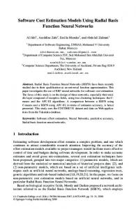
Figure 1: The geometry of IFW specimens (a) and meshed 2D axisymmetric model (b). Table 1: Properties of GH4169 superalloy used in simulations [20].
2. FE Model of IFW A two-dimensional (2D) axisymmetric model was built, as shown in Figure 1, employing a tubular specimen of 30 mm length, inner diameter of 15 mm, and thickness of 4 mm [17]. The mesh was created using quad elements with coupled displacement-temperature and the twist degree of freedom. The mesh size was chosen to change over the length of the specimen as shown in Figure 1(b), to reduce computation time while maintaining accuracy of the results. Due to the extensive interfacial deformation in the IFW process, the remeshing and map solution techniques were used to overcome excessive element distortion. The selfcontact option was also utilized to avoid early simulation abortion. Beside these, the actuator-sensor interaction and user element subroutines available in ABAQUS were adopted to measure transient flywheel rotational speed and upset. The available energy for heating is equal to the flywheel kinetic energy 𝐸0 , which can be expressed as 1 𝐸0 = 𝐽𝜔0 2 , 2
(1)
where 𝐽 is the flywheel moment of inertia and 𝜔0 the initial flywheel rotational speed. Hence, energy conversion from flywheel kinetic energy to heat during friction can be described as 𝐸𝑡+𝛿𝑡 = 𝐸𝑡 − 𝜔𝑡 𝛿𝑡 ∫ 𝑓𝑠 𝑟𝑑𝑆, 𝑆
(2)
where 𝜔𝑡 is the rotational speed, 𝛿𝑡 the time increment, 𝑟 the radial distance from the central axis, and 𝑆 the range of 𝑟. The nominal friction force 𝑓𝑠 can be divided into two stages to describe heat generation during the welding process according to Moal and Massoni [18]. When temperature is low, at the beginning of friction, friction stress is proportional to the prescribed pressure. With the friction continuing, interface temperature rises quickly and material flow stress
Temperature (∘ C) Young’s modulus (GPa) Thermal conductivity (W⋅m−1 ⋅K−1 ) Specific heat capacity (J⋅kg−1 ⋅K−1 )
20–1300 205–20 13.4–32.55 430–720
decreases rapidly, with friction behavior 𝑓𝑠 being defined as a thin Norton-Hoff layer subjected to a shear stress 𝜏, which can be written as 𝑉 𝜏 = −𝛼𝑝𝜇 𝑡 , 𝑉𝑡
(3)
where 𝛼 is a constant, 𝑝 the interface pressure, 𝑉𝑡 the relative sliding velocity, and 𝜇 the nominal coefficient of friction. The thermal conduction problem within the joint was solved using the 2D axisymmetric Fourier’s heat conduction equation. In addition, heat dissipation through convection was also considered and a constant heat transfer coefficient of 30 W⋅m−2 ⋅K−1 was adopted to prescribe the boundary condition between joint surfaces and the environment [19]. 2.1. Material Properties and Process Parameters. The temperature dependent material properties of the GH4169 superalloy were used in the finite element simulations. GH4169 according to the Chinese classifications, the same as Inconel 718, is a nickel-based superalloy with the following chemical composition by weight, 0.04% C, 0.13% Si, 0.10% Mn, 52.61% Ni, 18.95% Cr, 3.03% Mo, 5.14% Nb, 0.46% Al, 0.98% Ti, and balance Fe. The thermal and mechanical properties of GH4169 were drawn from literature [20], while some data at high temperatures were extrapolated from existing data, as shown in Table 1. The temperature dependent material flow stress data used in this simulation were drawn from literature [21, 22] as well as shown in Figure 2. In order to study the effects of axial pressure and initial rotational speed
Advances in Materials Science and Engineering
3
800 600 400 200 0 600
700
800
900
1000
1100
1200
1000 800 600 400 200
120 100
4
80 60 2
40 20
0
0
1300
1
2 Time (s)
3
4
5
0
Rotational speed Temperature Upset
Temperature (∘ C) 0.001 s−1 10 s−1 1000 s−1
6
140
Upset (mm)
Flow stress (MPa)
1000
400 MPa, 1.178 kg·m2 , 152.8 rad/s
160
1200 Rotational speed (rad/s)
Maximum interface temperature (∘ C)
1200
Figure 3: Variations of maximum interface temperature, rotational speed, and upset with welding time.
Figure 2: Temperature and strain rate dependent flow stress adopted in simulations.
Outer
t = 2s
Table 2: The IFW processing parameters studied. Parameter Moment of inertia (kg⋅m2 ) Axial pressure (MPa) Initial rotational speed (rad/s)
Value
Inner
1.178 250, 300, 350, 375, 400, 450, 475, 500 122.8, 132.8, 142.8, 152.8, 162.8
t = 2.5 s
on the IFW process, finite element simulations were carried out using parameters as shown in Table 2.
t = 4s
3. Simulation Results The simulation was conducted using the reported parameters of IFW of GH4169 superalloy tube by Yang et al. [17]. The moment of inertia, axial pressure, and initial rotational speed were 1.178 kg⋅m2 , 400 MPa, and 152.8 rad/s, respectively. The change of flywheel rotational speed is shown in Figure 3. It is clear that the rotational speed decreases linearly with time at the beginning of friction and decreases sharply just before the arrest of the flywheel. Meanwhile, there is no upset during the first 2 seconds of the process. Then, the upset increases almost linearly with friction time until 𝑡 = 4 s. It should be pointed out that the changing tendencies of these variables during IFW are relatively independent of the processing parameters, and the simulated final upset (6.2 mm) is comparable to experiments (about 5.7 mm) with an error of 8.7%. This validation enables the investigation of this parameter in the following sections and the effects of parameters on temperature field and upset as well. Figure 4 shows temperature contours and upset variation at different welding times. With frictional movement, the heated zone widens from the weld interface due to the heat generated by friction, plastic deformation, and the heat conducted into the specimen. After the interface temperature
NT11 1200.00 1101.67 1003.33 905.00 806.67 708.33 610.00 511.67 413.33 315.00 216.67 118.33 20.00 0.00
t = 4.3 s
Figure 4: Temperature contours and upset variation at different welding times.
reaches about 1100∘ C at about 2 s (see Figure 4), temperature remains steady, which may suggest that a thermal balance between heat generation and dissipation has formed at the interface. At this time, the plastic material near the interface begins to extrude under axial pressure and a flash is formed (Figure 4, 𝑡 = 2.5 s). It is also found that temperature contours and flash shape are asymmetric, which is the result of the nonuniform linear velocity along the radial direction of the
4
Advances in Materials Science and Engineering Input layer
of size m0 X1
Hidden layer of size N
Output layer of size one
𝜑1
For a strict interpolation, the interpolating surface (function 𝐹) should pass through all training data points. The RBF technique consists of choosing a function 𝐹 of the form
W1
𝑁
𝐹 (𝑥) = ∑ 𝑤𝑖 𝜑 (x − x𝑖 ) ,
(5)
𝑖=1
𝜑2
X2 . . .
XN
. . .
W2
where 𝑤𝑖 is the weight function at node 𝑥𝑖 and {𝜑(‖x − x𝑖 ‖) | 𝑖 = 1, 2, . . . , 𝑁} is a set of 𝑁 arbitrary (generally nonlinear) functions, known as radial basis functions as 2 x − x𝑖 ) , 𝑖 = 1, 2 . . . , 𝑁, 𝜑𝑖 (𝑥) = 𝜑 (x − x𝑖 ) = exp (− 2𝜎2 (6)
∑
y = F(x) WN
𝜑N
Figure 5: Structure of RBF neural network model.
specimen during welding which causes uneven heat generation. In addition, during IFW process, peak temperature at the interface is below the melting point of GH4169 (1260– 1340∘ C). When the welding time reaches about 4 s, the flash shape remains unchanged and the joint temperature begins to fall as shown in Figure 4. This can be clearly explained by studying the change of weld parameters, while the flywheel has a very small angular speed and the rotation completely stops at 4.3 s as shown in Figure 3. The upset remains constant after 4 s and the joint begins to cool down. The maximum interface temperature decreases quickly from about 1135∘ C to 980∘ C from 4 s to 4.3 s, and following this sharp decrease a less steep temperature decline follows. This sharp decrease of temperature is due to the fact that the thermal balance has been disturbed with quick heat dissipation by conduction from the interface to the cold end of specimen being much larger than the small or no heat generation at the interface at this stage.
where ‖x − x𝑖 ‖ denotes a norm that is usually Euclidean. The down data points x𝑖 ∈ 𝑅𝑚0 , 𝑖 = 1, 2, . . . , 𝑁 are taken to be the centers of the radial basis functions. According to the interpolation conditions, a set of simultaneous linear equations for the unknown coefficients (weights) of the expansion {𝑤𝑖 } are obtained 𝜑11 𝜑12 . . . 𝜑1𝑁 𝑤1 𝑑1 [ 𝜑21 𝜑22 . . . 𝜑2𝑁 ] [ 𝑤2 ] [ 𝑑2 ] [ ][ ] [ ] [ .. .. .. .. ] [ .. ] = [ .. ] , [ . . . . ][ . ] [ . ] [𝜑𝑁1 𝜑𝑁2 . . . 𝜑𝑁𝑁] [𝑤𝑁] [𝑑𝑁] where
𝜑𝑖𝑗 = 𝜑 (x𝑖 − x𝑗 ) ,
𝑇
d = [𝑑1 , 𝑑2 , . . . , 𝑑𝑁] ,
𝑖 = 1, 2 . . . , 𝑁.
(9)
𝑇
w = [𝑤1 , 𝑤2 , . . . , 𝑤𝑁] . The 𝑁-by-1 vectors d and w represent the desired response vector and linear weight vector, respectively, where 𝑁 is the size of the training sample. Let Φ denote an 𝑁-by-𝑁 matrix with elements 𝜑𝑖𝑗 as follows: 𝑁
Φ = {𝜑𝑖𝑗 }𝑖,𝑗=1 .
The RBF neural network is commonly used in functional approximation, spline interpolation, and mixed models [23]. The developed RBF neural network is composed of three layers of nodes as shown in Figure 5. The first layer is the input layer that feeds in input or training data to the second layer, which is a hidden layer. This second layer differs greatly from commonly used neural networks as each node represents a data cluster centered at a particular point and has a given radius. The final layer consists of only one node so as to output the second layer of nodes and yield a decision value. In fact, the upset prediction can be viewed as an interpolation problem, which can be stated as follows. Given a set of 𝑁 different points {x𝑖 ∈ 𝑅𝑚0 | 𝑖 = 1, 2, . . . 𝑁} and a corresponding set of 𝑁 real numbers {𝑑𝑖 ∈ 𝑅1 | 𝑖 = 1, 2, . . . 𝑁}, a function 𝐹 : 𝑅𝑁 → 𝑅1 is necessary to be found that satisfies the interpolation condition (4)
(8)
Let
4. Mathematical Prediction Model Settings
𝐹 (𝑥𝑖 ) = 𝑑𝑖 ,
𝑖, 𝑗 = 1, 2 . . . , 𝑁.
(7)
(10)
This is the interpolation matrix. Then (12) can be rewritten in a compact form Φw = b.
(11)
Assuming that Φ is nonsingular, then w = Φ−1 b.
(12)
Normally, training and testing points (𝑥𝑖𝑗 ) must be normalized within a range to enhance the efficiency of the model. In this paper, training and testing data are linearly normalized to a range of −1 to 1 by (13), and the output data are reverse normalized, 𝑥𝑖𝑗 =
2 × [𝑥𝑖𝑗 − min (𝑥𝑖𝑗 )] [max (𝑥𝑖𝑗 ) − min (𝑥𝑖𝑗 )]
− 1,
(13)
where 𝑥𝑖𝑗 is the normalized data and 𝑥𝑖𝑗 the training and testing points.
Advances in Materials Science and Engineering
5 102
Table 3: The final upsets under different IFW processing parameters.
350 375 400 350 375 400 250 300 350 375 400 450 475 500 250 300 350 375 400 450 475 500 250 300 350 375 400 450 475 500
122.8 122.8 122.8 132.8 132.8 132.8 142.8 142.8 142.8 142.8 142.8 142.8 142.8 142.8 152.8 152.8 152.8 152.8 152.8 152.8 152.8 152.8 162.8 162.8 162.8 162.8 162.8 162.8 162.8 162.8
101
Upset (mm) 0.13 0.73 1.36 1.40 2.15 2.85 0.01 1.18 2.99 3.78 4.53 5.76 6.31 6.86 0.51 2.80 4.73 5.51 6.20 7.47 8.06 8.56 2.12 4.70 6.46 7.24 7.99 9.18 9.86 11.50
5. Results and Discussion 30 sets of final upsets under different IFW processing parameters are shown in Table 3, which were used to build and train the RBF neural network. Following extensive optimization, it was found that an RBF neural network with 25 neurons in the hidden layer gives the best prediction of the upset. The performance mean squared error of this neural network model at the end of training is shown in Figure 6. The surface plot of the RBF predicted upset as a function of axial pressure and initial rotational speed is shown in Figure 7. Upset ranging from 0 to 15 mm can be clearly seen when axial pressure and initial rotational speed change from 200 MPa to 500 MPa and from 120 rad/s to 200 rad/s, respectively. This can be useful in parameter selection and upset prediction of IFW.
Training-blue
1 2 3 4 5 6 7 8 9 10 11 12 13 14 15 16 17 18 19 20 21 22 23 24 25 26 27 28 29 30
Performance is 0.0125123; goal is 0
100
10−1
10−2
0
5
10 15 25 epochs
20
25
Figure 6: Mean squared error of the network to predict upset of IFW.
14 15 Upset (mm)
No.
Parameters Axial pressure Initial rotational (MPa) speed (rad/s)
12 10
10
8 5
0 200 Ini t ia l
6 4 rot at
500 150 ion al s p ee
400
d(
rad
100 /s)
200
a) 300 (MP ure s s e l pr Axia
2 0
Figure 7: Surface plot of prediction results by RBF network.
To explore the feasibility of using such a network and the precision of its predictions, another 9 sets of FE simulated data, not used in the initial neural network training, were produced. The comparison between FE simulated upsets and RBF predicted ones and the relative error is shown in Table 4. It is clear that the RBF predicted values are close to the ones produced by the finite element model, with an acceptable absolute error of less than 0.3 mm. However, it also can be found that a frustrating large relative error of 8.16% exited at the condition of 300 MPa-147.8 rad/s, although a normal absolute error (0.16 mm) is obtained. This is probably because of the limited training data of the RBF network. From the surface plot of prediction results as shown in Figure 7, both the initial rotational speed and axial pressure greatly affect final upset. As the total welding heat for IFW should be converted from the flywheel kinetic energy, the initial flywheel kinetic energy is assumed to be a special parameter which affects the welding process. There is a proportional relationship between the flywheel kinetic energy,
6
Advances in Materials Science and Engineering Table 4: Comparison between FE simulated upsets and RBF predicted ones.
No.
Condition 300 MPa—147.8 rad/s 300 MPa—157.8 rad/s 300 MPa—167.8 rad/s 400 MPa—147.8 rad/s 400 MPa—157.8 rad/s 400 MPa—167.8 rad/s 500 MPa—147.8 rad/s 500 MPa—157.8 rad/s 500 MPa—167.8 rad/s 15
15
10
10
Absolute error (mm)
Relative error (%)
0.16 0.08 0.30 0.03 0.03 0.08 0.08 0.11 0.13
8.16 2.15 5.42 0.56 0.42 0.91 1.04 1.17 1.12
Upset (mm)
Upset (mm)
1 2 3 4 5 6 7 8 9
Upset (mm) FE simulated RBF predicted 1.96 2.12 3.72 3.64 5.53 5.23 5.38 5.35 7.09 7.06 8.75 8.83 7.72 7.64 9.43 9.54 11.63 11.5
5
0 1.5E4
5
2E4
2.5E4
3E4
3.5E4
Square of initial rotational speed ((rad/s) 2 ) 300 MPa 350 MPa 400 MPa 450 MPa
500 MPa + RBF predicted □ FEM simulated
Figure 8: Effect of square of initial rotational speed on upset predicted by RBF network.
and the square of initial rotational speed, with the effect of flywheel kinetic energy on the upset shown in Figure 8. There is very good agreement between RBF network predicted and FE simulated upset as shown in Table 4 and plotted in Figure 8. Furthermore, there exits a clear linear relationship between upset and the square of initial rotational speed which means that the final upset is almost predetermined by flywheel initial kinetic energy, when axial pressure is constant. However, it should also be noted that there is almost no upset under 300 MPa and when the square of initial rotational speed is smaller than 17689 (rad/s)2 (i.e., speed of 133 rad/s), suggesting that insufficient deformation develops at the interface. In a similar fashion, when axial pressure increases, there is also a low threshold of acceptable initial rotational speed necessary to produce the upset for a given axial pressure. 5.1. Effect of Axial Pressure on Upset. The effect of axial pressure on the upset was investigated and the results predicted
0 200
250 132.8 rad/s 142.8 rad/s 152.8 rad/s
300 350 400 Axial pressure (MPa)
450
500
162.8 rad/s 172.8 rad/s
Figure 9: Effect of axial pressure on upset predicted by RBF network.
by the RBF network are shown in Figure 9. One can see an exponentially increasing relationship between upset and axial pressure at different initial rotational speeds. It indicates that the upset changes more rapidly under relative low axial pressure which is not the case under relatively high axial pressure. Similar to the effect of initial rotational speed, the underlying mechanism of axial pressure on the upset can also be found in energy conversion. For example at the initial rotational speed of 142.8 rad/s, there is almost no upset under an axial pressure smaller than 265 MPa, while the upset reaches 5 mm under 420 MPa. According to the principle of IFW, the rotated flywheel is the sole mechanical energy source for welding, and the total energy for welding is up to its initial rotational speed. Thus the most appropriate expression for the upset change could be that the axial pressure affects significantly the efficiency of the conversion of mechanical energy to effective heat. Although the available flywheel kinetic energy is sufficient, it is difficult to heat rapidly (i.e., effective heat) at the interface and yield locally the workpiece under a relative low axial
Advances in Materials Science and Engineering
7 6
180 12.94
170
9.71
11.32
5 R2 = 0.963
8.09 4.85
160
6.47
Actual upset (mm)
Initial rotational speed (rad/s)
Map of upset
3.24 150 140 1.62
200
250
300
350
3 2 1
0.01
130
4
400
450
0
500
0
1
Axial pressure (MPa)
Figure 10: Parameter window based on the predicted upset by RBF network.
2 3 4 RBF predicted upset (mm)
5
6
Figure 11: Scatter diagram of RBF prediction versus actual upset of LFW.
14
5.2. Applications to LFW and CDFW. In published works [19, 25], simulations of CDFW and LFW have been conducted with FE models. The effects of processing parameters on temperature profile and upset have been explored in a systematic way. Based on these simulations, applications of RBF network on LFW and CDFW have been attempted. In literature [25], a 2D thermomechanically coupled finite element model of LFW TC4 titanium alloy was built and heat generation was produced due to friction between deformable and rigid surfaces. Using this model, the effect of most important parameters, such as oscillation frequency, amplitude, and friction pressure, on temperature profile and upset were examined. As a result, a mathematical upset prediction model was established in this study. A correlation coefficient (𝑅2 ) of 0.963 for the scatter diagram of RBF prediction versus actual upset (of the simulated results) was obtained as shown in Figure 11.
12
Actual upset (mm)
pressure. Therefore, in a similar fashion to critical initial rotational speed, there is a critical axial pressure for each initial rotational speed whose finding is necessary for process parameter selection. In fact, insufficient deformation (small upset) during IFW is generally considered as the reason for lacking of bonding, weak self-cleaning, and severe oxidation. According to Ates et al. [24], a serious decrease in the tensile strength of friction welded joints could be attributed to insufficient deformation under low axial pressure. Moreover, according to the results above, the RBF network predicts the critical welding parameters. To further develop the capability of the RBF network, the parameter prediction window was established based on the upset as shown in Figure 10. With a given upset, continuously changed welding parameters could be obtained from the prediction window for the studied workpiece in this study. Therefore, the RBF network could be helpful to predict and select processing parameters of IFW.
R2 = 0.998
10 8 6 4 2 0
0
2
4 6 8 10 RBF predicted upset (mm)
12
14
Figure 12: Scatter diagram of RBF prediction versus actual upset of CDFW.
In addition, the FE simulation of the CDFW process has also been developed using a 2D axisymmetric thermalmechanically coupled model, of a mild steel bar with a length of 150 mm and diameter of 20 mm. Furthermore, experimental and calculated upsets show an error of only 2.5%. Based on simulations using parameters provided in literature [19], a similar RBF regression analysis for the CDFW case has been obtained. The scatter diagram of RBF prediction versus actual upset (of the FE simulated results) shows a correlation coefficient of 0.998 in Figure 12. Therefore, the RBF neural network model can also be used to predict the outputs of LFW and CDFW with a significant accuracy.
6. Conclusions According to the analysis in this paper, the following conclusions can be drawn.
8
Advances in Materials Science and Engineering (1) The finite element modeling of IFW: a superalloy can well reveal the friction and upsetting processes. Based on these simulations, an RBF neural network was applied initially to establish a welding parameter prediction window based on the upset. (2) The developed RBF network model shows that there is a critical axial pressure for acceptable upset for each initial rotational speed. Similarly, there is also a critical initial rotational speed, that is, critical flywheel kinetic energy, for each axial pressure. (3) Depending on the energy conversion, the analysis of effects of IFW parameters on the upset indicates that the initial rotational speed determines the heat source and that axial pressure will significantly affect the heat accumulation at the weld interface. (4) Applications of the RBF network on LFW and CDFW were also developed, with correlation coefficients for LFW and CDFW being 0.963 and 0.998, respectively, suggesting that RBF is an effective prediction method for friction welding.
[8]
[9]
[10]
[11]
[12]
Conflict of Interests The authors declare that they do not have a direct relation with any commercial identities that might lead to a conflict of interests for any of them.
[13]
[14]
Acknowledgments The authors would like to thank for financial support the National Natural Science Foundation of China (51005180 and 61065009) and the 111 Project (B08040).
[15]
References
[16]
[1] M. Maalekian, “Friction welding—critical assessment of literature,” Science and Technology of Welding and Joining, vol. 12, no. 8, pp. 738–759, 2007. [2] F. M. Ham and I. Kostanic, Principles of Neurocomputing for Science and Engineering, McGraw-Hill, New York, NY ,USA, 1 edition, 2001. [3] S. C. Juang, Y. S. Tarng, and H. R. Li, “A comparison between the back-propagation and counter-propagation networks in the modeling of the TIG welding process,” Journal of Materials Processing Technology, vol. 75, no. 1–3, pp. 54–62, 1998. [4] B. Chan, J. Pacey, and M. Bibby, “Modelling gas metal arc weld geometry using artificial neural network technology,” Canadian Metallurgical Quarterly, vol. 38, no. 1, pp. 43–51, 1999. [5] J. Y. Jeng, T. F. Mau, and S. M. Leu, “Prediction of laser butt joint welding parameters using back propagation and learning vector quantization networks,” Journal of Materials Processing Technology, vol. 99, no. 1, pp. 207–218, 2000. [6] D. S. Nagesh and G. L. Datta, “Prediction of weld bead geometry and penetration in shielded metal-arc welding using artificial neural networks,” Journal of Materials Processing Technology, vol. 123, no. 2, pp. 303–312, 2002. [7] K. H. Christensen, T. Sørensen, and J. K. Kristensen, “Gas metal arc welding of butt joint with varying gap width based on neural
[17]
[18]
[19]
[20]
[21]
[22]
networks,” Science and Technology of Welding and Joining, vol. 10, no. 1, pp. 32–43, 2005. P. Ghanty, M. Vasudevan, D. P. Mukherjee et al., “Artificial neural network approach for estimating weld bead width and depth of penetration from infrared thermal image of weld pool,” Science and Technology of Welding and Joining, vol. 13, no. 4, pp. 395–401, 2008. M. Vasudevan, V. Arunkumar, N. Chandrasekhar, and V. Maduraimuthu, “Genetic algorithm for optimisation of ATIG welding process for modified 9Cr-1Mo steel,” Science and Technology of Welding and Joining, vol. 15, no. 2, pp. 117–123, 2010. G. Casalino, S. J. Hu, and W. Hou, “Deformation prediction and quality evaluation of the gas metal arc welding butt weld,” Proceedings of the Institution of Mechanical Engineers B, vol. 217, no. 11, pp. 1615–1622, 2003. S. Pal, S. K. Pal, and A. K. Samantaray, “Artificial neural network modeling of weld joint strength prediction of a pulsed metal inert gas welding process using arc signals,” Journal of Materials Processing Technology, vol. 202, no. 1–3, pp. 464–474, 2008. B. Acherjee, S. Mondal, B. Tudu, and D. Misra, “Application of artificial neural network for predicting weld quality in laser transmission welding of thermoplastics,” Applied Soft Computing Journal, vol. 11, no. 2, pp. 2548–2555, 2011. H. Okuyucu, A. Kurt, and E. Arcaklioglu, “Artificial neural network application to the friction stir welding of aluminum plates,” Materials and Design, vol. 28, no. 1, pp. 78–84, 2007. P. Sathiya, S. Aravindan, A. N. Haq, and K. Paneerselvam, “Optimization of friction welding parameters using evolutionary computational techniques,” Journal of Materials Processing Technology, vol. 209, no. 5, pp. 2576–2584, 2009. S. S. Kumaran, S. Muthukumaran, and S. Vinodh, “Optimization of friction welding of tube to tube plate using an external tool by hybrid approach,” Journal of Alloys and Compounds, vol. 509, no. 6, pp. 2758–2769, 2011. E. Boldsaikhan, E. M. Corwin, A. M. Logar, and W. J. Arbegast, “The use of neural network and discrete Fourier transform for real-time evaluation of friction stir welding,” Applied Soft Computing Journal, vol. 11, no. 8, pp. 4839–4846, 2011. J. Yang, S. N. Lou, Y. Zhou, J. M. Yan, and W. Q. Shi, “The dynamic recrystallization properties of superalloy GH4169 inertia friction welding joint,” Journal of Aeronautical Materials, vol. 22, no. 2, pp. 8–11, 2002 (Chinese). A. Moal and E. Massoni, “Finite element simulation of the inertia welding of two similar parts,” Engineering Computations, vol. 12, no. 6, pp. 497–512, 1995. W. Y. Li and F. F. Wang, “Modeling of continuous drive friction welding of mild steel,” Materials Science and Engineering A, vol. 528, no. 18, pp. 5921–5926, 2011. L. W. Zhang, J. B. Pei, Q. Z. Zhang et al., “The coupled fem analysis of the transient temperature field during inertia friction welding of GH4169 alloy,” Acta Metallurgica Sinica, vol. 20, no. 4, pp. 301–306, 2007. M. S. Lewandowski and R. A. Overfelt, “High temperature deformation behavior of solid and semi-solid alloy 718,” Acta Materialia, vol. 47, no. 18, pp. 4695–4710, 1999. J. J. DeMange, V. Prakash, and J. M. Pereira, “Effects of material microstructure on blunt projectile penetration of a nickel-based super alloy,” International Journal of Impact Engineering, vol. 36, no. 8, pp. 1027–1043, 2009.
Advances in Materials Science and Engineering [23] M. P. Phaniraj and A. K. Lahiri, “The applicability of neural network model to predict flow stress for carbon steels,” Journal of Materials Processing Technology, vol. 141, no. 2, pp. 219–227, 2003. [24] H. Ates, M. Turker, and A. Kurt, “Effect of friction pressure on the properties of friction welded MA956 iron-based superalloy,” Materials and Design, vol. 28, no. 3, pp. 948–953, 2007. [25] W. Y. Li, T. Ma, and J. Li, “Numerical simulation of linear friction welding of titanium alloy: effects of processing parameters,” Materials & Design, vol. 31, no. 3, pp. 1497–1507, 2010.
9
Journal of
Nanotechnology Hindawi Publishing Corporation http://www.hindawi.com
Volume 2014
International Journal of
International Journal of
Corrosion Hindawi Publishing Corporation http://www.hindawi.com
Polymer Science Volume 2014
Hindawi Publishing Corporation http://www.hindawi.com
Volume 2014
Smart Materials Research Hindawi Publishing Corporation http://www.hindawi.com
Journal of
Composites Volume 2014
Hindawi Publishing Corporation http://www.hindawi.com
Volume 2014
Journal of
Metallurgy
BioMed Research International Hindawi Publishing Corporation http://www.hindawi.com
Volume 2014
Nanomaterials
Hindawi Publishing Corporation http://www.hindawi.com
Volume 2014
Submit your manuscripts at http://www.hindawi.com Journal of
Materials Hindawi Publishing Corporation http://www.hindawi.com
Volume 2014
Journal of
Nanoparticles Hindawi Publishing Corporation http://www.hindawi.com
Volume 2014
Nanomaterials Journal of
Advances in
Materials Science and Engineering Hindawi Publishing Corporation http://www.hindawi.com
Volume 2014
Journal of
Hindawi Publishing Corporation http://www.hindawi.com
Volume 2014
Journal of
Nanoscience Hindawi Publishing Corporation http://www.hindawi.com
Scientifica
Hindawi Publishing Corporation http://www.hindawi.com
Volume 2014
Journal of
Coatings Volume 2014
Hindawi Publishing Corporation http://www.hindawi.com
Crystallography Volume 2014
Hindawi Publishing Corporation http://www.hindawi.com
Volume 2014
The Scientific World Journal Hindawi Publishing Corporation http://www.hindawi.com
Volume 2014
Hindawi Publishing Corporation http://www.hindawi.com
Volume 2014
Journal of
Journal of
Textiles
Ceramics Hindawi Publishing Corporation http://www.hindawi.com
International Journal of
Biomaterials
Volume 2014
Hindawi Publishing Corporation http://www.hindawi.com
Volume 2014