Use Case Point Approach Based Software Effort Estimation using ...

arXiv:1401.3069v2 [cs.SE] 15 Jan 2014

Use Case Point Approach Based Software Effort Estimation using Various Support Vector Regression Kernel Methods Shashank Mouli Satapathya , Santanu Kumar Rathb a

Department of Computer Science and Engineering, National Insitutte of Technology Rourkela, Rourkela 769008 India, Contact: [email protected] b

Department of Computer Science and Engineering, National Insitutte of Technology Rourkela, Rourkela 769008 India, Contact: [email protected] The job of software effort estimation is a critical one in the early stages of the software development life cycle when the details of requirements are usually not clearly identified. Various optimization techniques help in improving the accuracy of effort estimation. The Support Vector Regression (SVR) is one of several different soft-computing techniques that help in getting optimal estimated values. The idea of SVR is based upon the computation of a linear regression function in a high dimensional feature space where the input data are mapped via a nonlinear function. Further, the SVR kernel methods can be applied in transforming the input data and then based on these transformations, an optimal boundary between the possible outputs can be obtained. The main objective of the research work carried out in this paper is to estimate the software effort using use case point approach. The use case point approach relies on the use case diagram to estimate the size and effort of software projects. Then, an attempt has been made to optimize the results obtained from use case point analysis using various SVR kernel methods to achieve better prediction accuracy. Keywords : Object Oriented Analysis and Design, Software Effort Estimation, Support Vector Regression, Use Case Point Approach.

1. INTRODUCTION

ment life cycle plays a vital role for determining whether a project is feasible in terms of a costbenefit analysis [5,6]. The Use Case Point (UCP) model relies on the use case diagram to estimate the effort of a given software product. UCP helps in providing more accurate effort estimation from design phase of software development life cycle. UCP is measured by counting the number of use cases and the number of actors, each multiplied by its complexity factors. Use cases and actors are classified into three categories. These include simple, average and complex. The determination of the complexity value (simple, average or complex) of use cases is determined by the number of transactions per use case. The UCP model has widely been used in the last decade [7], yet it has several limitations. One of the limitations is that the software effort equation is not well accepted by software estimators because it assumes that the relation-

Proper software effort estimation is the foremost activity adopted in every software development life cycle. Several features offered by OO programming concept such as Encapsulation, Inheritance, Polymorphism, Abstraction, Cohesion and Coupling play an important role to manage the development process [1,2]. Currently used software development effort estimation models such as, COCOMO and Function Point Analysis (FPA), do not consistently provide accurate project cost and effort estimates [3]. These techniques have been proven unsatisfactory for estimating cost and effort because the lines of code (LOC) and function point (FP) are both used for procedural oriented paradigm [4]. Both of them have certain limitations. The LOC is dependent on the programming language and the FPA is based on human decisions. Hence effort estimation during early stage of software develop1

2 ship between software effort and size is linear. In this paper, various kernel methods based support vector regression is introduced to tackle the limitations of the UCP model and to enhance prediction accuracy of the software effort estimation. The result obtained from these support vector regression techniques based effort estimation model is then compared with other models in order to assess performance of those models. 2. RELATED WORK This section presents related work regarding the use case point based effort estimation approach and support vector regression model. A. Issha et al., [8] reports on the development of three novel use case model based software cost estimation methods such as use case rough estimation method, use case patterns estimation method, and object points extraction estimation method. The accuracy of the proposed methods has been investigated using a wide spectrum of software projects. Ali B. Nassif et al., [9] presents a novel regression model to estimate the software effort based on the use case point size metric. They proposed an effort equation that takes into consideration the non-linear relationship between software size and software effort, as well as the influences of project complexity and productivity. Results show that the software effort estimation accuracy can be improved by 16.5%. Ali B. Nassif et al., [10] extended this process by applying mamdani fuzzy inference system with regression model to enhance the estimation accuracy and found 10% improvement in the result. Ali B. Nassif et al., [11] also applied sugeno fuzzy inference system with regression model to enhance the estimation accuracy and found 11% improvement in the MMRE result. Ali B. Nassif et al., [12] propose a novel Artificial Neural Network (ANN) to predict software effort from use case diagrams based on the Use Case Point (UCP) model with the help of 240 data points and found a competitive result with respect to other regression model. Ali B. Nassif et al., [13] also present some techniques using fuzzy logic and neural networks to improve the accuracy of the use case points method and obtained an improvement up to 22%.

Satapathy S M, et al., Ali B. Nassif et al., [14] uses a Treeboost (Stochastic Gradient Boosting) model to predict software effort based on the Use Case Point method using 84 data points and obtain promising results. Adriano L.I. Oliveira [15] provides a comparative study on support vector regression (SVR), radial basis function neural networks (RBFNs) and linear regression for estimation of software project effort. The experiment is carried out using NASA project datasets and the result shows that SVR performs better than RBFN and linear regression. Petrˆ onio L. Braga et al., [16] have proposed and investigated the use of a genetic algorithm approach for selecting an optimal feature subset and optimizing SVR parameters simultaneously aiming to improve the precision of the software effort estimates. E. Kocaguneli et al., [17] have investigated non-uniform weighting through kernel density estimation and found that nonuniform weighting through kernel methods cannot outperform uniform weighting Analogy Based Estimation (ABE). Bilge Bakele et al., [18] propose a model that uses machine learning methods and evaluate the model on public data sets and data gathered from software organization. From analysis, it is found out that the usage of any one model cannot produce the best results for software effort estimation. 3. METHODOLOGY USED The following methodologies are used in this paper to calculate the effort of a software product. 3.1. Use Case Point Approach The Use Case Point (UCP) model was proposed by Gustav Karner in 1993 [19]. This method is an extension of Function Point Analysis and Mk II Function Point Analysis (an adaptation of FPA mainly used in the UK), and is based on the same philosophy as these methods. An early estimate of effort based on use cases can be made when there is some understanding of the problem domain, system size and architecture at the stage at which the estimate is made. The block diagram shown in Figure 1 explains the steps to calculate the class point. The use case point approach can be imple-

3

UCP Based Software Effort Estimation using Various SVR Kernel Methods Use Case Diagram

Classification of Actors and Use Cases

Calculation of Weights and Points

Calculation of TCF and EF

Final Use Case Point Evaluation

Figure 1. Steps to Calculate Use Case Point

all. Counting number of transactions can be done by counting the use case steps. The use case is considered as Simple, when it uses a simple user interface and touches only a single database entity. The use case is considered as Average, when it involves more interface design and touches 2 or more database entities. Similarly the use case is Complex, when it involves a complex user interface or processing and touches 3 or more database entities. Use case complexity is then defined and weighted in the following manner:

Table 2 Use Case Weighting Factors Use Case Type

mented using the following steps: 3.1.1. Classification of Actors and Use Cases The first step is to classify the actors as simple, average or complex. A simple actor represents another system with a defined Application Programming Interface, API, an average actor is another system interacting through a protocol such as TCP/IP, and a complex actor may be a person interacting through a GUI or a Web page. A weighting factor is assigned to each actor type in the following manner:

Table 1 Actor Weighting Factors

Actor Type

Weighting Factor

Simple

1

Average

2

Complex

3

Similarly each use case is defined as simple, average or complex, depending on number of transactions in the use case description, including secondary scenarios. A transaction is a set of activities, which is either performed entirely, or not at

No. of Transactions Type

Weighting Factor

Simple

= 7

15

3.1.2. Calculation of Weights and Points The total Unadjusted Actor Weights (UAW) is calculated by counting how many actors there are of each kind (by degree of complexity), multiplying each total by its weighting factor, and adding up the products. Similarly each type of use case is then multiplied by the weighting factor, and the products are added up to get the Unadjusted Use Case Weights (UUCW). Then the UAW is added to the UUCW to get the Unadjusted Use Case Points (UUCP). U U CP = U AW + U U CW

(1)

3.1.3. Calculation of TCF and EF The UUCP are adjusted based on the values‘assigned to a number of technical and environmental factors shown in Tables 3 and 4. Each factor is assigned a value between 0 and 5 depending on its assumed influence on the project. A rating of 0 means the factor is irrelevant for this project and 5 means it is essential. The adjustment factors are multiplied by the unadjusted use case points to produce the adjusted use case points, yielding an estimate of

4

Satapathy S M, et al.,

Table 3 Technical Factors

sum called the EFactor. The following equation gives EF value:

Factor

Description

Weight

T1

Distributed System

2

T2

Response Adjectives

2

T3

End-user Efficiency

1

T4

Complex Processing

1

T5

Reusable Code

1

T6

Easy to Install

0.5

T7

Easy to Use

0.5

T8

Portable

2

T9

Easy to Change

1

T10

Concurrent

1

T11

Security Features

1

T12

Access for Third Parties

1

T13

Special Training Required

1

EF = 1.4 + (−0.03 ∗ EF actor)

3.1.4. Final Use Case Point Calculation The final adjusted use case points (UCP) are calculated as follows: U CP = U U CP ∗ T CF ∗ EF

Description

Weight

F1

Familiar with RUP

1.5

F2

Application Experience

0.5

F3

Object-oriented Experience

1

F4

Lead Analyst Capability

0.5

F5

Motivation

1

F6

Stable Requirements

2

F7

Part-time Workers

-1

F8

Difficult Programming Language

2

the size of the software. The Technical Complexity Factor (TCF) is calculated by multiplying the value of each factor (T1- T13) by its weight and then adding all these numbers to get the sum called the TFactor. The following formula is applied to find TCF: T CF = 0.6 + (0.01 ∗ T F actor)

(4)

The final use case point value is then taken as input argument to support vector regression model to calculate estimated normalized effort.

Table 4 Environment Factors Factor

(3)

(2)

The Environmental Factor (EF) is calculated by multiplying the value of each factor (F1-F8) by its weight and adding the products to get the

3.2. Support Vector Regression Technique Support Vector Machines (SVM) are learning machines implementing the structural risk minimization inductive principle to obtain a good generalization on a limited number of learning patterns. A version of SVM for regression was proposed by Vladimir N. Vapnik et al. [20] in 1996. This method is called as support vector regression (SVR). Generally any neural networks suffers from two major drawbacks. First of all neural networks often converge on local minima rather than global minima. Secondly neural networks often over-fit which means, if training on a pattern goes on too long, then it may consider noise as part of pattern. SVR doesnt suffer from either of these two drawbacks and have the advantages due to which it can be successfully used for regression task. Suppose, for a given training data (x1 , y1 ), . . . , (xl , yl ), where x ∈ Rn denotes the space of the input patterns and y ∈ R denotes its corresponding target value. The goal of regression is to find the function f (x) that best models the training data. For the case of nonlinear regression, f (x) = hw, φ(x)i + b, where φ is a nonlinear function which maps the input space to a higher (maybe infinite) dimensional feature space and h., .i denotes the dot product in Rn . In SVR, the weight vector ‘w’ and the threshold ‘b’ are chosen

UCP Based Software Effort Estimation using Various SVR Kernel Methods to optimize the following problem [21]. minw,b,ξ,ξ∗ = (1/2wT w + C

Pl

i=1 (ξi

5

– -g: width parameter γ – -p: ǫ for epsilon-SV regression.

+ ξi∗ ))

• linear: K(xi , xj ) = xTi xj .

The value of parameter ‘s’ ranges from 0 to 5 and the default value is 0. For epsilon-SV regression, the parameter ‘s’ is assigned with value 3. The ‘t ’ value ranges from 0 to 3 for different types of kernel. In this case, the value can be 0, 1, 2 or 3 for linear, polynomial, RBF and sigmoid kernel respectively. The default value for ‘t ’ is 2. Similarly, the value of parameter ‘c’ will be calculated as the difference between maximum and minimum value of actual effort used to train the model. The default value is 1. The parameter ‘g’ value shows width parameter i.e., it set γ in various kernel function. The default value is 1. Lastly, the value of parameter ‘p’ set the ǫ in loss function of epsilon-SVR. The default value for parameter ‘p’ is 0.1. The use of these tunable parameters helps in accurately estimating the predicted effort using various SVR kernel methods.

• polynomial: K(xi , xj ) = (γxTi xj + r)d , γ > 0.

4. PROPOSED APPROACH

subject to (hw, φ(xi )i + b) − yi ≤ ǫ + ξi , yi − (hw, φ(xi )i + b)+ ≤ ǫ + ξi∗ , ξi , ξi∗ ≥ 0.

(5)

C > 0 is the penalty parameter of the error term. ξ and ξ ∗ are called slack variables and measure the cost of the errors on the training points. ξ measures deviations exceeding the target value by more than ǫ and ξ ∗ measures deviations which are more than ǫ, but below the target value [15]. K(xi , xj ) = φ(xTi φ(xj )) is called the kernel function. There are basically four kernels. These are:

• Radial Basis Function (RBF): K(xi , xj ) = exp(−γ kxi − xj k2 ), γ > 0.

• sigmoid: K(xi , xj ) = tanh(γxTi xj + r).

Here γ, r, and d are kernel parameters. In epsilonSV regression [21], the goal is to find a function f (x) that has at most ǫ deviation from the actually obtained targets yi for all the training data, and at the same time is as flat as possible. In other words, errors less than ǫ are ignored and considered as zero. But errors larger than ǫ are measured by variable ξ and ξ ∗ . The following tunable parameters [22] have been used while implementing support vector regression. • param: This is a string which specifies the model parameters. For regression model, a typical parameter string may look like, ‘-s 3 -t 2 -c 20 -g 64 -p 1’ where – -s: svm type, – -t: kernel type – -c: penalty parameter C of epsilon-SV regression.

The proposed approach is based on eight-four data set used in the article [14]. The use of this data set intends to evaluate software development effort and validate the practicability of improvement. The use of such data in the validation process has provided initial experimental evidence of the effectiveness of the UCP. These data are used to develop the support vector regression based software effort estimation model. The block diagram shown in Figure 2 displays the proposed steps used to determine the predicted effort using various kernel based support vector regression technique. To calculate the effort of a given software project, basically the following steps have been used. Steps in Effort Estimation 1. Calculation of Use Case Point: After collecting the data from previously developed projects, the use case point (UCP) has been calculated from the use case diagram using the steps proposed by Karner [19]. 2. Scaling of Data Set: The generated UCP

6

Satapathy S M, et al., vided into two parts i.e., training set & test set. The training set is used for model estimation, whereas the test set is used only for estimating the predicted effort of the final model. While selecting a model of optimal complexity, divide the training set into a two parts i.e., learning set & validation set. The learning set is used to estimate model parameters, whereas the validation set is used for selecting an optimal model complexity. This step is implemented using 5-fold cross validation.

Calculation of Use Case Point

Scaling of Data Set

Division of Data Set

Performing Parameters & Model Selection

4. Performing Parameters & Model Selection: The model which provides the least value than the other generated models based on the minimum validation error criteria has been selected to perform other operations.

Selection of Parameters

Selection of Best Model

Training of Selected Model

Calculation of Error and Prediction Accuracy

Figure 2. Proposed Steps Used for Effort Estimation using Various SVR Kernel Methods

value in Step-1 has been used as input arguments and has been scaled within the range [0,1]. Let X be the dataset and x is an element of the dataset, then the scaled value of x can be calculated as : x′ =

x − min(X) max(X) − min(X)

(6)

where x′ = Scaled value of x within the range [0,1]. min(X) = the minimum value for the dataset X. max(X) = the maximum value for the dataset X. If max(X) is equal to min(X), then Normalized(x) is set to 0.5. 3. Division of Data Set: The data set is di-

5. Selection of Parameters: The tunable parameters are selected to find the best value of C and γ using a five fold crossvalidation procedure . 6. Selection of Best Model: Based on the minimum validation error, the best model has been selected and the corresponding value of γ and ǫ value is found out. 7. Training of Selected Model: The final model selected based on best parameter of C, ǫ and γ are trained using all training samples. The output of this step is the trained SVM model providing predicted response values for test inputs. 8. Calculation of Error and Prediction Accuracy: The performance of the model is checked by calculating Root Mean Square Error (RMSE), Mean Magnitude of Relative Error (MMRE) and Prediction Accuracy (PRED) for test sample and training sample. The graphs generated using obtained results indicate visual comparison of the parameters. The above steps are followed to implement the SVR based effort estimation model using various kernel methods. Finally, a comparison of results obtained using various kernels based SVR effort

7

UCP Based Software Effort Estimation using Various SVR Kernel Methods estimation model has been presented to assess their performances. 5. EXPERIMENTAL DETAILS In this paper to implement the proposed approaches, eighty four dataset is being used which is also used by Ali B. Nasif et al. [14]. The detail description about the data set has already been provided in proposed approach section. The data set is divided into different subsets for the training, testing and validation purpose. First of all, every fifth data out of those two data sets, is extracted for testing purpose and rest data will be used for training purpose. Then the training data has been partitioned into the learning / validation sets. The 5-fold data partitioning is done on the training data by the following strategy : For partition 1: Samples 1, 6, 11, ... have been used as validation samples and the remaining as learning samples For partition 2: Samples 2, 7, 12, ... have been used as validation samples and the remaining as learning samples . . . For partition 5: Samples 5, 10, 15, ... have been used as validation samples and the remaining as learning samples. After partitioning data into learning set and validation set, the model selection for ǫ and γ is performed using 5-fold cross-validation process. In this paper, to perform model selection, the ǫ and γ values are varied over a range. The γ value ranges from 2−7 to 27 and ǫ value ranges from 0 to 5. Hence, ninty number of models will be generated to perform model selection operation. Table 5 and 6 show the validation error of ninty numbers of models generated for CP1 using SVR linear kernel and SVR polynomial kernel respectively based on the value of ǫ and γ. For SVR Linear kernel, 0.0009 value has been chosen as the minimum validation error. Hence based on the minimum validation error, the best model is C = 0.99891, γ = 2−7 (0.0078) and ǫ = 0. Similarly for SVR Polynomial kernel, 0.0057 value

Table 5 Validation Errors Obtained Using SVR Linear Kernel for UCP ǫ=0

1

2

3

4

5

γ = 2−7

0.0009

0.2054

0.2054

0.2054

0.2054

0.2054

2−6

0.0009

0.2054

0.2054

0.2054

0.2054

0.2054

2−5

0.0009

0.2054

0.2054

0.2054

0.2054

0.2054

2−4

0.0009

0.2054

0.2054

0.2054

0.2054

0.2054

2−3

0.0009

0.2054

0.2054

0.2054

0.2054

0.2054

2−2

0.0009

0.2054

0.2054

0.2054

0.2054

0.2054

2−1

0.0009

0.2054

0.2054

0.2054

0.2054

0.2054

20

0.0009

0.2054

0.2054

0.2054

0.2054

0.2054

21

0.0009

0.2054

0.2054

0.2054

0.2054

0.2054

22

0.0009

0.2054

0.2054

0.2054

0.2054

0.2054

23

0.0009

0.2054

0.2054

0.2054

0.2054

0.2054

24

0.0009

0.2054

0.2054

0.2054

0.2054

0.2054

25

0.0009

0.2054

0.2054

0.2054

0.2054

0.2054

26

0.0009

0.2054

0.2054

0.2054

0.2054

0.2054

27

0.0009

0.2054

0.2054

0.2054

0.2054

0.2054

Table 6 Validation Errors Obtained Using SVR Polynomial Kernel for UCP ǫ=0

1

2

3

4

5

γ = 2−7

0.0434

0.2054

0.2054

0.2054

0.2054

0.2054

2−6

0.0434

0.2054

0.2054

0.2054

0.2054

0.2054

2−5

0.0434

0.2054

0.2054

0.2054

0.2054

0.2054

2−4

0.0434

0.2054

0.2054

0.2054

0.2054

0.2054

2−3

0.0431

0.2054

0.2054

0.2054

0.2054

0.2054

2−2

0.0409

0.2054

0.2054

0.2054

0.2054

0.2054

2−1

0.0257

0.2054

0.2054

0.2054

0.2054

0.2054

20

0.0059

0.2054

0.2054

0.2054

0.2054

0.2054

21

0.0058

0.2054

0.2054

0.2054

0.2054

0.2054

22

0.0058

0.2054

0.2054

0.2054

0.2054

0.2054

23

0.0058

0.2054

0.2054

0.2054

0.2054

0.2054

24

0.0058

0.2054

0.2054

0.2054

0.2054

0.2054

25

0.0058

0.2054

0.2054

0.2054

0.2054

0.2054

26

0.0058

0.2054

0.2054

0.2054

0.2054

0.2054

27

0.0057

0.2054

0.2054

0.2054

0.2054

0.2054

has been chosen as the minimum validation error. Hence based on the minimum validation error, the best model is C = 0.99891, γ = 27 (128) and ǫ = 0. Similarly, Table 7 and 8 show the validation error of ninty numbers of models generated for

8


Table 7 Validation Errors Obtained Using SVR RBF Kernel for UCP ǫ=0

1

2

3

4

5

γ = 2−7

0.0370

0.2054

0.2054

0.2054

0.2054

0.2054

2−6

0.0312

0.2054

0.2054

0.2054

0.2054

0.2054

2−5

0.0213

0.2054

0.2054

0.2054

0.2054

0.2054

2−4

0.0105

0.2054

0.2054

0.2054

0.2054

0.2054

2−3

0.0044

0.2054

0.2054

0.2054

0.2054

0.2054

2−2

0.0008

0.2054

0.2054

0.2054

0.2054

0.2054

2−1

0.0008

0.2054

0.2054

0.2054

0.2054

0.2054

20

0.0007

0.2054

0.2054

0.2054

0.2054

0.2054

21

0.0007

0.2054

0.2054

0.2054

0.2054

0.2054

22

0.0010

0.2054

0.2054

0.2054

0.2054

0.2054

23

0.0011

0.2054

0.2054

0.2054

0.2054

0.0897

24

0.0012

0.2054

0.2054

0.2054

0.2054

0.2054

25

0.0016

0.2054

0.2054

0.2054

0.2054

0.2054

26

0.0020

0.2054

0.2054

0.2054

0.2054

0.2054

7

0.0020

0.2054

0.2054

0.2054

0.2054

0.2054

2

Table 8 Validation Errors Obtained Using SVR Sigmoid Kernel for UCP γ=2

−7

ǫ=0

1

2

3

4

5

0.0401

0.2054

0.2054

0.2054

0.2054

0.2054

2−6

0.0370

0.2054

0.2054

0.2054

0.2054

0.2054

2−5

0.0311

0.2054

0.2054

0.2054

0.2054

0.2054

2−4

0.0210

0.2054

0.2054

0.2054

0.2054

0.2054

2

−3

0.0099

0.2054

0.2054

0.2054

0.2054

0.2054

2

−2

0.0046

0.2054

0.2054

0.2054

0.2054

0.2054

2−1

0.0014

0.2054

0.2054

0.2054

0.2054

0.2054

20

0.0054

0.2054

0.2054

0.2054

0.2054

0.2054

21

0.1014

0.2054

0.2054

0.2054

0.2054

0.2054

22

0.6041

0.2054

0.2054

0.2054

0.2054

0.2054

23

2.0331

0.2054

0.2054

0.2054

0.2054

0.2054

24

5.0454

0.2054

0.2054

0.2054

0.2054

0.2054

25

7.5381

0.2054

0.2054

0.2054

0.2054

0.2054

26

10.1991

0.2054

0.2054

0.2054

0.2054

0.2054

27

11.0733

0.2054

0.2054

0.2054

0.2054

0.2054

CP1 using SVR RBF kernel and SVR Sigmoid kernel respectively based on the value of ǫ and γ. For VR RBF kernel, 0.0007 value has been chosen as the minimum validation error. Hence based on the minimum validation error, the best model is C = 0.99891, γ = 20 (1) and ǫ = 0. Similarly

for SVR Sigmoid kernel, 0.0014 value has been chosen as the minimum validation error. Hence based on the minimum validation error, the best model is C = 0.99891, γ = 2−1 (0.5) and ǫ = 0. Finally based on model parameters value, the model has been again trained and tested using training and testing data set respectively to estimate the effort. 5.1. Performance Measures The performance of the various models can be evaluated by using the following criteria [23]: • The Mean Square Error (MSE) measures the average of the squares of the errors and is calculated as: M SE =

PN

i=1

2

(yi − y¯) N

(7)

where yi = Actual Effort of ith test data. y¯ = Predicted Effort of ith test data. N = Total number of data in the test set. • The Mean Magnitude of Relative Error (MMRE) can be achieved through the summation of MRE over N observations M M RE =

N X |yi − y¯| 1

yi

(8)

• The Root Mean Square Error (RMSE) is just the square root of the mean square error. RM SE =

√ M SE

(9)

• The Normalized Root Mean Square(NRMS) can be calculated by dividing the RMSE value with standard deviation of the actual effort value for training data set. N RM S =

RM SE std(Y )

(10)

where Y is the actual effort for testing data set.

9

UCP Based Software Effort Estimation using Various SVR Kernel Methods

While using the MMRE and PRED in evaluation, good results are implied by lower values of MMRE and higher value of PRED. After implementing the support vector regression based model using four different kernel methods for software effort estimation, the following results have been generated. SVR Linear Kernel Result for UCP: Param: -s 3 -t 0 -c 0.9989 -g 0.0078 -p 0 * Mean Squared Error (MSE TEST) = 0.0026 (regression) * Squared correlation coefficient = 0.9932 (regression) * NRMS Test = 0.2431 SVR Polynomial Kernel Result for UCP: Param: -s 3 -t 1 -c 0.9989 -g 128 -p 0 * Mean Squared Error (MSE TEST) = 0.0018 (regression) * Squared correlation coefficient = 0.9003 (regression) * NRMS Test = 0.4588 SVR RBF Kernel Result for UCP: Param: -s 3 -t 2 -c 0.9989 -g 1 -p 0 * Mean Squared Error (MSE TEST) = 0.0030 (regression) * Squared correlation coefficient = 0.9881 (regression) * NRMS Test = 0.2822 SVR Sigmoid Kernel Result for UCP: Param: -s 3 -t 3 -c 0.9989 -g 0.5 -p 0 * Mean Squared Error (MSE TEST) = 0.0034 (regression) * Squared correlation coefficient = 0.9920 (regression) * NRMS Test = 0.2764 The squared correlation coefficient (r2 ) also known as the coefficient of determination is one of the best approaches for evaluating the strength of a relationship. It is the proportion of variance in

actual effort that can be accounted for by knowing use case point value for training data set. In the output generated, it is quite clearly mentioned that the squared correlation coefficient value for different kernels is very high (greater than 0.9). Hence it can be concluded that there is a strong positive correlation between the use case point and the predicted effort required to develop the software i.e., a minor change in the use case point value results in significant change in the predicted effort value.

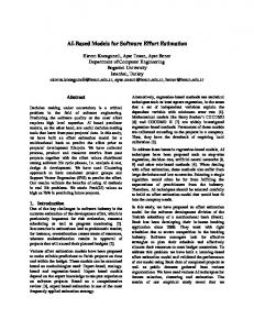
1 0.9 Training Examples Testing Examples Prediction

0.8 0.7

Effort (PM)

• The Prediction Accuracy (PRED) can be calculated as: PN |yi − y¯| )) ∗ 100 (11) P RED = (1 − ( i=1 N

0.6 0.5 0.4 0.3 0.2 0.1 0

0.2

0.4

0.6

0.8

1

Use Case Point (UCP)

Figure 3. SVR Linear Kernel based Effort Estimation Model for UCP

The proposed model generated using the SVR linear, polynomial, RBF and sigmoid kernel for UCP have been plotted based on the training and testing sample data set as shown in Figure 3, 4, 5 and 6. The graphs show the variation of predicted effort value with respect to its corresponding use case point value. In these graphs, it is clearly shown that the data points are very little dispersed than the regression line. Hence the correlation is higher. While comparing the dispersion of data points from the predicted model in the above graphs for UCP, it is clearly visible that for SVR RBF kernel based UCP model, the data points are less dispersed than other models. Hence, the models exhibit less error values and higher prediction accuracy values.

10


1

1

0.9

0.9 Training Examples Testing Examples Prediction

0.8

0.7

Effort (PM)

Effort (PM)

0.7 0.6 0.5 0.4

0.6 0.5 0.4

0.3

0.3

0.2

0.2

0.1 0

Training Examples Testing Examples Prediction

0.8

0.1 0.2

0.4

0.6

0.8

1

0

0.2



0.9 Training Examples Testing Examples Prediction

Effort (PM)

0.7

0.5 0.4 0.3 0.2 0.1 0.2

0.4

0.6

0.8

1


Actual Effort

0.6

0

0.6

Table 9 Comparison of Efforts obatined using various SVR kernel methods for UCP

1

0.8

0.4


0.8

1


SVR Linear Effort

SVR Polynomial Effort

SVR RBF Effort

1

0.0100

0.0030

0.0090

0.0047

0.0018

2

0.0031

-0.0035

0.0090

0.0010

SVR Sigmoid Effort -0.0054

3

0.0024

-0.0003

0.0090

0.0028

-0.0018

4

0.0015

0.0027

0.0090

0.0045

0.0015

5

0.0061

0.0042

0.0090

0.0054

0.0031

6

0.0050

0.0056

0.0090

0.0063

0.0047

7

0.0064

0.0086

0.0090

0.0080

0.0080

8

0.0083

0.1902

0.0090

0.0089

0.0096

9

0.0082

0.1791

0.0090

0.0107

0.0129

10

0.0200

0.1791

0.0090

0.0141

0.0191

11

0.0356

0.1791

0.0091

0.0243

0.0366

12

0.0568

0.1791

0.0092

0.0299

0.0457

13

0.0352

0.1791

0.0093

0.0377

0.0581

14

0.0464

0.1791

0.0095

0.0455

0.0701

15

0.0553

0.1791

0.0103

0.0656

0.0990

16

0.1383

0.1791

0.0246

0.1818

0.2357

17

0.3945

0.1791

0.2926

0.6128

0.6052


for testing out of a data set of eighty four data.

6. COMPARISON

Table 10 Comparison of Prediction Accuracy Values of Related Works

On the basis of results obtained, the estimated effort using various SVR kernel methods are compared. The result shows that effort estimation using SVR RBF kernel based model gives less values of MMRE and higher prediction accuracy values than those obtained using other SVR kernel methods. Table. 9 shows the comparison of actual effort with an estimated effort by various SVR kernel methods for UCP on the seventeen data taken

Related Papers

Technique Used

Prediction Accuracy

A. Issha et al. [8]

3 Novel UCP model

67%

Ali B. Nasif et al. [14]

TreeBoost Model

88%


Artificial Neural Network Model

90.27%


Regression Model

95.8%

Table 10 provides a comparative study of the results obtained by some articles mentioned in the

UCP Based Software Effort Estimation using Various SVR Kernel Methods related work section. The performance of techniques used in those articles have been compared by measuring their prediction accuracy (PRED) values. Result shows that, a maximum of 95% prediction accuracy is achieved using regression analysis technique for UCP. Finally, the results obtained in related work section is compared with results of proposed approaches, which is shown in Table 11. The results obtained using proposed technique shows improvement in the prediction accuracy value.

Table 11 Comparison of errors and prediction accuracy values obtained using various SVR kernel methods for UCP MMRE

PRED

SVR Linear Kernel

0.5438

97.7421%

SVR Polynomial Kernel

1.0003

97.4089%

SVR RBF Kernel

0.3857

98.0188%

SVR Sigmoid Kernel

0.6049

97.3931%

11

ware product. Then the results obtained have been optimized using four different support vector regression kernel methods. At the end of the study, a comparative analysis of the generated results has been presented in order to assess their accuracy. While comparing the results with the results provided in the related work section, it can be concluded that the results obtained from proposed models outperform the results generated by models given in related work section. Similarly, while comparing the results obtained using various SVR kernel methods, it can be concluded that for UCP, RBF kernel based support vector regression technique outperformed other three kernel methods. The computations for above procedure have been implemented and membership functions generated using MATLAB. This can be further analyzed and proved if real data for Use Point Approach is available. This approach can also be extended by using some other soft computing techniques such as Particle Swarm Optimization (PSO) and Genetic Algorithm (GA). REFERENCES

Table 11 displays the final comparison of MMRE and PRED values for different SVR kernel methods. While comparing the obtained results with the results provided in related work section i.e., in Table 10, it can be observed that the obtained results from proposed models provide better prediction accuracy values than the results obtained from models given in related work section. Similarly, the results obtained from different proposed models show that effort estimation using SVR RBF kernel gives less values of MMRE and higher values of prediction accuracy than those obtained using other SVR kernel methods. 7. CONCLUSION The Use Case Point Approach is one of the different effort estimation models that can be used for effort estimation of softwares developed using object oriented methodology, because it is simple, fast, accurate to a certain degree. In this paper, first the use case point approach is used to estimate the effort involved in developing a soft-

1. M. Carbone and G. Santucci. Fast&&serious: a uml based metric for effort estimation. In Proceedings of the 6th ECOOP Workshop on Quantitative Approaches in Object-Oriented Software Engineering (QAOOSE’02), pages 313–322, 2002. 2. Nasib S. Gill and Sunil Sikka. New complexity model for classes in object oriented system. SIGSOFT Softw. Eng. Notes, 35(5):1–7, October 2010. 3. Zhiwei Xu and Taghi M Khoshgoftaar. Identification of fuzzy models of software cost estimation. Fuzzy Sets and Systems, 145(1):141– 163, 2004. 4. J.E. Matson, B.E. Barrett, and J.M. Mellichamp. Software development cost estimation using function points. Software Engineering, IEEE Transactions on, 20(4):275– 287, 1994. 5. SG MacDonell and AR Gray. A comparison of modeling techniques for software development effort prediction. In Proceedings of fourth International Conference on

12

6.

7.

8.

9.

10.

11.

12.

13.

Satapathy S M, et al., Neural Information Processing, pages 869– 872, Dunedin, New Zealand, 1998. SpringerVerlag. Kevin Strike, Khaled El Emam, and Nazim Madhavji. Software cost estimation with incomplete data. Software Engineering, IEEE Transactions on, 27(10):890–908, 2001. Mel Damodaran and A Washington. Estimation using use case points. Computer Science Program. Texas–Victoria: University of Houston. Sd, 2002. Ayman Issa, Mohammed Odeh, and David Coward. Software cost estimation using usecase models: A critical evaluation. In Information and Communication Technologies, 2006. ICTTA’06. 2nd, volume 2, pages 2766– 2771. IEEE, 2006. Ali Bou Nassif, Danny Ho, and Luiz Fernando Capretz. Regression model for software effort estimation based on the use case point method. In 2011 International Conference on Computer and Software Modeling, pages 117– 121, 2011. Ali Bou Nassif, Luiz Fernando Capretz, and Danny Ho. A regression model with mamdani fuzzy inference system for early software effort estimation based on use case diagrams. In Third International Conference on Intelligent Computing and Intelligent Systems, pages 615–620, 2011. Ali Bou Nassif, Luiz Fernando Capretz, and Danny Ho. Estimating software effort based on use case point model using sugeno fuzzy inference system. In Tools with Artificial Intelligence (ICTAI), 2011 23rd IEEE International Conference on, pages 393–398. IEEE, 2011. Ali Bou Nassif, Luiz Fernando Capretz, and Danny Ho. Estimating software effort using an ann model based on use case points. In Machine Learning and Applications (ICMLA), 2012 11th International Conference on, volume 2, pages 42–47. IEEE, 2012. Ali Bou Nassif. Enhancing use case points estimation method using soft computing techniques. Journal of Global Research in Computer Science, 1(4), 2010.

14. Ali Bou Nassif, Luiz Fernando Capretz, Danny Ho, and Mohammad Azzeh. A treeboost model for software effort estimation based on use case points. In Machine Learning and Applications (ICMLA), 2012 11th International Conference on, volume 2, pages 314–319. IEEE, 2012. 15. Adriano LI Oliveira. Estimation of software project effort with support vector regression. Neurocomputing, 69(13):1749–1753, 2006. 16. Petrˆ onio L Braga, Adriano LI Oliveira, and Silvio RL Meira. A ga-based feature selection and parameters optimization for support vector regression applied to software effort estimation. In Proceedings of the 2008 ACM symposium on Applied computing, pages 1788–1792. ACM, 2008. 17. Ekrem Kocaguneli, Tim Menzies, and Jacky W Keung. Kernel methods for software effort estimation. Empirical Software Engineering, 18(1):1–24, 2013. 18. Bilge Baskeles, Burak Turhan, and Ay¸se Bener. Software effort estimation using machine learning methods. In Computer and information sciences, 2007. iscis 2007. 22nd international symposium on, pages 1–6. IEEE, 2007. 19. Gustav Karner. Resource estimation for objectory projects. Objective Systems SF AB, 17, 1993. 20. Harris Drucker, Chris JC Burges, Linda Kaufman, Alex Smola, and Vladimir Vapnik. Support vector regression machines. Advances in neural information processing systems, pages 155–161, 1997. 21. Alex J Smola and Bernhard Sch¨ olkopf. A tutorial on support vector regression. Statistics and computing, 14(3):199–222, 2004. 22. Chih-Chung Chang and Chih-Jen Lin. LIBSVM: A library for support vector machines. ACM Transactions on Intelligent Systems and Technology, 2:27:1–27:27, 2011. Software available at http://www.csie.ntu.edu.tw/~cjlin/libsvm. 23. Tim Menzies, Zhihao Chen, Jairus Hihn, and Karen Lum. Selecting best practices for effort estimation. Software Engineering, IEEE Transactions on, 32(11):883–895, 2006.

UCP Based Software Effort Estimation using Various SVR Kernel Methods S M Satapathy did his MCA from Silicon Institute of Technology and M.Tech in Computer Science & Engineering from KIIT University, Bhubaneswar, India. Currently he is pursuing his PhD in Computer Science and Engineering at National Institute of Technology, Rourkela, India. His areas of interest are Software Cost Estimation, Program Slicing. S K Rath is a Professor in the Department of Computer Science and Engineering, NIT Rourkela since 1988. His research interests are in Software Engineering, System Engineering, Bioinformatics & Management. He has published a large number of papers in international journals and conferences in these areas. He is a Senior Member of the IEEE, USA and ACM, USA and Petri Net Society, Germany.

13