computation with multiple files by each processor writing out its own portion simulation ..... Name of a reservoir domain, as specified in data block ROCKS.
LBNL-315E
User’s Guide for TOUGH2-MP A Massively Parallel Version of the TOUGH2 Code
Keni Zhang, Yu-Shu Wu, and Karsten Pruess
Earth Sciences Division Lawrence Berkeley National Laboratory May 2008
2
ABSTRACT TOUGH2-MP is a massively parallel (MP) version of the TOUGH2 code, designed for computationally efficient parallel simulation of isothermal and nonisothermal flows of multicomponent, multiphase fluids in one, two, and three-dimensional porous and fractured media. In recent years, computational requirements have become increasingly intensive in large or highly nonlinear problems for applications in areas such as radioactive waste disposal, CO2 geological sequestration, environmental assessment and remediation, reservoir engineering, and groundwater hydrology. The primary objective of developing the parallel-simulation capability is to significantly improve the computational performance of the TOUGH2 family of codes. The particular goal for the parallel simulator is to achieve orders-of-magnitude improvement in computational time for models with ever-increasing complexity.
TOUGH2-MP is designed to perform parallel simulation on multi-CPU computational platforms. An earlier version of TOUGH2-MP (V1.0) was based on the TOUGH2 Version 1.4 with EOS3, EOS9, and T2R3D modules, a software previously qualified for applications in the Yucca Mountain project, and was designed for execution on CRAY T3E and IBM SP supercomputers. The current version of TOUGH2-MP (V2.0) includes all fluid property modules of the standard version TOUGH2 V2.0. It provides computationally efficient capabilities using supercomputers, Linux clusters, or multi-core PCs, and also offers many user-friendly features. The parallel simulator inherits all process capabilities from V2.0 together with additional capabilities for handling fractured media from V1.4.
This report provides a quick starting guide on how to set up and run the TOUGH2-MP program for users with a basic knowledge of running the (standard) version TOUGH2 code, The report also gives a brief technical description of the code, including a discussion of parallel methodology, code structure, as well as mathematical and numerical methods used. To familiarize users with the parallel code, illustrative sample problems are presented.
3
www.tough2.com
4
TABLE OF CONTENTS
ABSTRACT 1. INTRODUCTION .......................................................................................................... 7 2. REQUIREMENTS AND CODE INSTALLATION .................................................... 10 2.1 Hardware and Software Requirements ................................................................... 10 2.2 Code Compilation and Installation ......................................................................... 11 3. METHODOLOGY AND CODE ARCHITECTURE .................................................. 15 3.1 Grid Domain Partitioning and Gridblock Reordering ............................................ 16 3.2 Organization of Input and Output Data .................................................................. 19 3.3 Assembly and Solution of Linearized Equation Systems ....................................... 20 3.4 Communication between Processors ...................................................................... 22 3.5 Updating Thermophysical Properties ..................................................................... 22 3.6 Program Structure and Flow Chart ......................................................................... 23 4. DESCRIPTION OF INPUT FILES .............................................................................. 26 4.1 Preparation of Input Data........................................................................................ 26 4.2 Input File Format .................................................................................................... 26 4.3 Input Formats for MESHMAKER.......................................................................... 51 4.3.1 Generation of Radially Symmetric Grids ........................................................ 52 4.3.2 Generation of Rectilinear Grids ....................................................................... 55 4.3.3 MINC Processing for Fractured Media............................................................ 56 4.4 Special Input Requirements for TOUGH2-MP ...................................................... 58 4.5 Output from TOUGH2-MP..................................................................................... 68 5. USER FEATURES ....................................................................................................... 73 6. SAMPLE PROBLEMS................................................................................................. 74 6.1 Unsaturated Flow Simulation ................................................................................. 75 6.2 Contaminant Transport Simulation......................................................................... 76 6.3 Investigation of CO2 Convection Mixing ............................................................... 78 6.4 Large-scale two-phase water and hydrogen flow simulation ................................. 81 7. CONCLUDING REMARKS........................................................................................ 90 ACKNOWLEDGEMENT ................................................................................................ 91 REFERENCES ................................................................................................................. 93 APPENDIX A. RUNNING TOUGH2-MP ON MULTIPLE-CORE PCs ....................... 98 APPENDIX B. RELATIVE PERMEABILITY FUNCTIONS...................................... 100 APPENDIX C. CAPILLARY PRESSURE FUNCTIONS ............................................ 105
5
6
1. INTRODUCTION TOUGH2 (Pruess, 1987; Pruess, 1991; Pruess et al., 1999) is a general-purpose numerical simulation program for multi-dimensional, multiphase, multicomponent fluid flows, heat transfer and contaminant transport in porous and fractured media. It has been used worldwide for geothermal reservoir engineering, nuclear waste isolation, environmental assessment and remediation, and modeling flow and transport in variably saturated media. The TOUGH2-MP code, a massive parallel version of the TOUGH2 code, was originally developed on CRAY T3E and IBM SP supercomputers (Elmroth et al., 2001; Zhang et al. 2001; Wu et al., 2002, Zhang, 2003). Since then, the parallel code has been improved in many ways by optimizing memory use, improving communication schemes, and including more fluid property modules (Zhang et al. 2003, 2006). Since its development, the parallel code has been successfully applied to large-scale simulations with up to several million gridblocks (e.g., Zhang et al., 2003a, Zhang et al. 2004, Yamamoto et al., 2007, Senger et al., 2008).
The original TOUGH2 code, an enhanced version of the TOUGH code (Pruess, 1987), was first released in 1991 (Pruess, 1991) with five basic EOS modules. The enhanced version 2.0 of the TOUGH2 code was made available to the public in 1999 and included additional fluid property modules (Pruess et al., 1999). The parallel version TOUGH2MP V1.0 (Zhang, 2003) was developed based on the original TOUGH2 V1.4 simulator (Wu et al., 1999; Wu, 1999), i.e., by implementing parallel computing algorithms into the V1.4 code. In early efforts at developing parallel simulation capabilities, Elmroth et al. (2001) developed a parallel prototype scheme for the TOUGH2 code for Massively Parallel Processor (MPP) computers. Zhang et al. (2001 and 2003) made further improvements in distributing memory requirements and improving computational efficiency for solving extremely large reservoir simulation problems with millions of gridblocks. As compared with the previous version of the parallel code, the current version of TOUGH2-MP Version 2.0, has been significantly improved in the efficiency of its
7
communication schemes. The improvements in the new version are achieved through reductions in the number of small-size messages and in the size of large messages. To achieve a faster nonlinear iteration converging speed, at each Newton iteration information exchanges across sub-domain boundaries are limited to primary variables only, while all secondary variables are updated locally, using primary variables for the sub-domain. Furthermore, the message-exchange speed is enhanced by using nonblocking communications during both linear and nonlinear iterations. We have also modified the AZTEC parallel linear-equation solver (Tuminaro et al., 1999) to nonblocking communication. All these improvements result in the current version of TOUGH2-MP being faster and more scalable than its predecessor.
In performing a parallel simulation, the TOUGH2-MP code first subdivides a simulation domain, defined by an unstructured grid of a TOUGH2 mesh, into a number of subdomains using the partitioning algorithm from the METIS software package (Karypsis and Kumar, 1998). The parallel code then relies on the MPI (Message-Passing Interface; Message Passing Forum, 1994) for its parallel implementation. Parallel simulations are run as multiple processes on a few or many processors simultaneously.
Each
process/processor is in charge of one portion of the simulation domain for updating thermophysical properties, assembling mass and energy balance equations, solving liner equation systems, and performing other local computations. The local linear equation systems are solved in parallel by multiple processors with the Aztec linear solver package. Although each processor solves the linearized equations of subdomains independently, the entire linear equation system is solved together by all processors collaboratively via communication between neighboring processors during each Newton iteration step.
Although TOUGH2-MP V2.0 was designed for parallel computing using multiple processors, the code can provide significant gains in computational efficiency even for single processor machines by executing nominally parallel processes in sequential mode. When multiple processors are available, it may be advantageous to partition a simulation domain into more subdomains than available processors, making the program execution partially sequential. This somewhat surprising finding can be explained from the behavior
8
of the linear equation solution in the subdomains, which for large problems consumes most of the numerical work in a simulation. By partitioning into a larger number of subdomains, we obtain a larger number of smaller linear algebra problems, which can be solved more efficiently than a smaller number of larger problems. However, with increasing number of processes there also is increased overhead from message passing, which leads to optimal performance for some "intermediate" level of domain partitioning. Another advantage of running parallel processes partially sequentially is that memory requirements may be reduced, so that larger problems with more grid blocks can be tackled.
The numerical scheme of the TOUGH2 code is based on the integral finite-difference (IFD) method (Narasimhan and Witherspoon, 1976; Pruess, 1987, 1991). In the TOUGH2 formulation, conservation equations, involving mass of air, water and chemical components as well as thermal energy, are discretized in space using the IFD method. Time is discretized fully implicitly using a first-order backward finite difference scheme. The resulting discrete finite-difference equations for mass and energy balances are nonlinear and solved simultaneously using the Newton/Raphson iterative scheme. All these numerical schemes are adopted by TOUGH2-MP. The parallel code also inherits all the process capabilities of the TOUGH2 code, including descriptions of the thermodynamics and thermophysical properties of the multiphase flow system. In addition, FORTRAN 90 features are introduced to TOUGH2-MP, such as dynamic memory allocation, array operation, matrix manipulation, and replacing “common blocks” (used in the original TOUGH2) with modules. All new subroutines are written in FORTRAN 90. Program units imported from the original TOUGH2 remain in FORTRAN 77, except for the use of data modules. The current version of TOUGH2-MP includes following modules: EOS1, EOS2, EOS3, EOS4, EOS5, EOS7, EOS7R, EOS8, EOS9, ECO2N, EWASG, and T2R3D. Other members of the TOUGH family including TMVOC and TOUGH+HYDRATE (Zhang et al., 2008) have also been parallelized.
The parallelization of TOUGH2 improves modeling capabilities significantly in terms of problem size and simulation time. The code demonstrates excellent scalability. Test
9
examples show that a linear or super-linear speedup can be obtained on typical Linux clusters as well as on supercomputers. Because the TOUGH2-MP parallel simulator was developed from an existing mature code, it inherits not only simulation functions from the original code, but also all other features, including input/output format, error handling, and improvements for code stability. These features provide robustness of the parallel code and ease of use for the user community of the original code, using identical input data, mesh and output files. Moreover, the domain decomposition approach and parallel computation enhance model simulation capabilities in terms of problem size and complexity to a level that cannot be reached by single-CPU codes. By using the parallel simulator, multi-million gridblock problems can be run on a typical Linux cluster with several tens to hundreds of processors to achieve ten to hundred times improvement in computational time or problem size. Our tests indicate that the parallel simulator allows much larger problems to be solved by multiple-process simulation even with a singleprocessor computer. This surprising result can be understood in terms of efficiency gains from decomposing one large linear algebra problem into a series of smaller ones, which produces super-linear speedup. The growing availability of multi-core CPUs will make parallel processing on PCs far more attractive.
This report provides a quick reference guide for utilizing the TOUGH2-MP code. The users are supposed to have basic knowledge of the original TOUGH2 family of codes. In particular, this report together with the TOUGH2 V2.0 User’s Guide provides sufficient information for users to apply TOUGH2-MP to subsurface flow simulation problems. A detailed technical description of the physical processes modeled, and the mathematical and numerical methods used in the code can be found in the user’s guide for TOUGH2 Version 2.0 (Pruess et al., 1999).
2. REQUIREMENTS AND CODE INSTALLATION 2.1 Hardware and Software Requirements TOUGH2-MP has been tested on IBM and CRAY supercomputers, Linux clusters, Macs, and multi-core PCs under different operating systems. It has been successfully compiled
10
using g95, and Fortran compilers from Intel, IBM, and the Portland Group. The code requires 64-bit arithmetic (8 byte word length for floating point numbers) for successful execution. TOUGH2-MP can be run on any shared- or distributed-memory multiple CPU computer system on which MPI is installed. The code has been run on LAM/MPI, OPEN MPI, and MPICH2. The total computer memory required by TOUGH2-MP depends on the problem size. For a given problem, memory requirement is split among the processors used for the simulation. The code automatically distributes memory requirements to all processors based on the partitioning of the domain. All major arrays are dynamically allocated according to the numbers of local gridblocks and connections assigned by domain partitioning to each processor. As a result, larger problems can be solved using more processors on a distributed memory computer system. For example, by far the largest array used in TOUGH2-MP is “PAR”, the array for storage of secondary variables. Its size in bytes (using 8-byte real data) is
M=(NPH*(NB+NK)+2)*(NEQ+1)*NEL*8
(2.1)
Here the parameters are the total number of fluid phases NPH, secondary parameter number NB, component number NK, and gridblock number NEL. If NPH=3, NB=8, NK=3, NEQ=4, NEL=106, the total memory requirement for this array is about 1400 MB. If 64 processors are used to solve this problem, each processor requires about 22 MB of memory for this array. One of the critical bottlenecks of memory requirement is during the reading of the MESH file through the master processor. This bottleneck is avoided by a reading-distributing strategy that replaces the original MESH with two files. Detailed discussion of this approach is provided in Section 4.4.
2.2 Code Compilation and Installation The source code of TOUGH2-MP consists of 10 FORTRAN files:
Compu_Eos.f,
Data_DD.f , Input_Output.f , Main_Comp.f , Mem_Alloc.f, Mesh_Maker.f, MULTI.f, Paral_Subs.f,
TOUGH2.f,
Utility_F.f , as listed in Table 2-1. Two library files
11
libmetis.a and libaztec.a are also needed for compiling the parallel program. The two library files are generated by compiling the METIS and AZTEC software packages. Different EOS modules need different “Compu_Eos.f” files. Compilation of each module should use its own “Compu_Eos.f” file. In addition, the EOS9, T2R3D and TMVOC modules require their own special modified core files.
Table 2-1 List of program files of the TOUGH2-MP source code File name Main_Comp.f
Functions Main program for time stepping and
Note Required
parallel running control. Data_DD.f
Data declaration and distribution
Required
Input_Output.f
Input and output
Required
Compu_Eos.f
EOS Modules and satellite functions
Required
Mem_Alloc.f
Memery allocation
Required
Mesh_Maker.f
Meshmaker
Optional
MULTI.f
Jacobian assembly
Required
Para_Subs.f
Parallelization related subroutines
Required
TOUGH2.f
Program entrance
Required
Utility_F.f
Utility subroutines
Required
libmetis.a
Compiled METIS functions
Library file
libaztec.a
Compile AZTEC functions
Library file
Compilation and installation can be done through the following steps: 1. Download METIS at: http://www-users.cs.umn.edu/~karypis/metis/metis/download.html 2. Compile METIS in the computer system where TOUGH2-MP will be installed. 3. Download AZTEC at: http://www.cs.sandia.gov/CRF/aztec1.html 4. Compile AZTEC in the computer system where TOUGH2-MP will be installed. (Guides for compiling METIS and AZTEC are provided with the downloaded packages.)
12
5. Transfer the core “tough2-mp_v2.0.tar.gz” and the selected EOS module “eosx.tar.gz” from the installation medium to your working directory. 6. Use gunzip to unzip the files and then use the tar command to untar the archived files and directories as follows: gunzip tough2-mp_2.0.tar.gz tar –xvf tough2-mp_2.0.tar gunzip eosx.tar.gz tar –xvf eosx.tar Two directories named “tough2-mp” and “eosx” will be created under the current working directory for the core and the selected EOS module respectively. Source files, make scripts, and installation test input files will be located in the subdirectories. Two additional subdirectories are created under the directory tough2-mp: ~/tough2mp/partition/ and ~/tough2-mp/utilities/. 7. Copy az_aztecf.h and libaztec.a from ~/aztec/lib and libmetis.a from ~/metis-4.0 to the subdirectories where source codes are located (~/tough2-mp/src). Copy additional source file(s) and makefile from selected module package (~/eosx) to this subdirectory. Replace all files at ~/tough2-mp/src by files with the same name at the ~/eosx/. The libaztec.a and libmetis.a files are created when Aztec and Metis is successfully compiled. 8. The “makefile” for three different compilers are provided: IBM, INTEL and PORTLAND GROUP. You can choose the one most close to your compiler. In the “makefile”, a wrapper compiler, mpif90, was specified for compiling the source codes. The user may need to change the compiler name to the one installed in the computer system by editing the file “makefile” at the line containing “FC=mpif90”. The user may also need to specify the path for MPI “include” and “library” files. Figure 2-1 shows a “makefile” for creating a TOUGH2-MP/EOS3 executable using PORTLAND GROUP Fortran 90. 9. Type “make” under the ~/tough2-mp/src/ subdirectory to compile the code. The executable file “t2eosx-mp” will be created. After compilation, type “make clean” to clean all intermediate files.
13
10. In order to successfully build TOUGH2-MP, the c and FORTRAN compilers used for compiling the MPI system, AZTEC, METIS and TOUGH2-MP source codes must be compatible. A Fortran 90 or higher version must be used for FORTRAN source code compilation.
# for clusters FC = mpif90 FFLAGS = -O -r8 -i4 # The following specifies the files used for the "standard version" OBJS = Data_DD.o Mem_Alloc.o MULTI.o Main_Comp.o TOUGH2.o \ Compu_Eos.o Input_Output.o Mesh_Maker.o \ Paral_Subs.o Utility_F.o \ LIBS = libmetis.a libaztec.a tough2: $(OBJS) $(FC) -o t2eos3-mp $(FFLAGS) $(OBJS) $(LIBS) clean: rm -f *.o *.mod
Figure 2-1. A makefile for TOUGH2-MP compilation
If “invalid communicator” or other communication problems are encountered during running the executable, user may try following: 1. Copy ~/tough2-mp/utilities/md_wrap_mpi_c.c to ~/aztec/lib to replace the original one. 2. Recompile AZTEC and then use the new library libaztec.a to recompile the TOUGH2-MP executable. If you have difficulty using the linear solver “AZ_gmres”, you may try the following: 1. Copy ~/tough2-mp/utilities/la_dlaic1.f to ~/aztec/lib to replace the original one. 2. Recompile AZTEC and then use the new library libaztec.a to recompile the TOUGH2-MP executable. One may get additional speedup by using non-blocking communication version AZTEC by performing the following steps:
14
1. Copy ~/tough2-mp/utilities/az_comm.c and ~/tough2-mp/utilities/az_matvec_mult.c to ~/aztec/lib to replace the original files. 2. Recompile AZTEC and then use the new library libaztec.a to recompile the TOUGH2-MP executable. The library file “libmetis.a” contains subroutines of the METIS package for partitioning irregular graphs and meshes. For reducing the requirement of computer memory, we use 4-byte integer for all large integer arrays in TOUGH2-MP. The corresponding arrays in METIS must also be a 4-byte integer. This can be implemented by simply removing the line of “#define IDXTYPE_INT” in head file “struct.h” of the METIS source code. The library file “libaztec.a” provides subroutines for solving linear equation systems in parallel.
3. METHODOLOGY AND CODE ARCHITECTURE Domain decomposition methods (DDM) are used as a divide and conquer strategy for solving large or time-consuming problems. The idea behind this approach is to divide the computational domain into a series of subdomains. Through the local solutions on the subdomains, a global solution is formed. Solutions for subdomains can be sought simultaneously. Therefore this approach is suitable for parallel computations as long as the computational work can be evenly distributed. The TOUGH2-MP numerical computational scheme is based on a fully implicit formulation with Newton iteration. The resulting linearized equations are solved by a parallel linear solver from the AZTEC package (Tuminaro et al., 1999). AZTEC includes a number of Krylov iterative methods, such as conjugate gradient (CG), generalized minimum residual (GMRES) and stabilized biconjugate gradient (BiCGSTAB). Fully implicit scheme has been proven to be the most robust numerical approach in modeling multiphase flow and heat transfer in reservoirs over the past several decades. For a typical simulation with the fully implicit scheme and Newton iteration, such as in the TOUGH2 run, the most time-consuming steps of the execution consist of three parts: (1) updating thermophysical parameters, (2) assembling the Jacobian matrix, and (3) solving the linearized system of equations. Consequently, one of the most important aims of a parallel simulation is to distribute computational time
15
for these three parts. In addition, a parallel scheme must take into account domain decomposition, grid node/element reordering, data input and output optimizing, and efficient message exchange between processors. These important parallel-computing strategies and implementation procedures are discussed below.
3.1 Grid Domain Partitioning and Gridblock Reordering Developing an efficient and effective method for partitioning unstructured grid domains is a critical step for a successful parallel-computing scheme. Firstly, to achieve better numerical performance, parallel simulations require the distribution of gridblocks evenly to different processing elements (PEs) or processors, i.e., the number of gridblocks assigned to each PE should be roughly the same. Secondly, the number of connections across domain bounds is minimized. The goal of the first requirement is to balance computational work among the processors. The goal of the second requirement is to minimize the time consumed in communication between processors (resulting from the estimation of the coupling terms or connections across the domain bounds by different processors).
In a TOUGH2-MP simulation, a model domain, or grid, is represented by a set of one-, two- or three-dimensional gridblocks (elements), and the interfaces between any two gridblocks are represented by connections. The entire grid system is treated as an unstructured grid. From the connection information, an adjacency matrix can be constructed. The adjacency or connection structure of the model meshes is stored in a compressed storage format (CSR).
The adjacency structure of storing the model grid can be described as follows: In the CSR format, the adjacency structure of a global-mesh domain with n gridblocks and m connections is represented by two arrays, xadj and adj. The xadj array has a size of n+1, whereas the adj array has a size of 2m. Assuming that element numbering starts from 1, the adjacency list of element i is stored in an array adj, starting at index xadj(i) and ending at index xadj(i+1)-1. That is, for each element i, its adjacency list is stored in the consecutive locations in the array adj, and the array xadj is used to point to where it
16
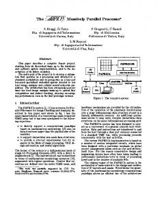
begins and where it ends. Figure 3-1a shows the connection of a 12-element domain; Figure 3-1b illustrates its corresponding CSR-format arrays.
We utilize one of the three partitioning algorithms provided by the METIS software package (version 4.0) (Karypsis and Kumar, 1998) for the grid domain partitioning. The three algorithms are denoted, respectively, as the K-way, the VK-way, and the Recursive partitioning algorithm. K-way is used for partitioning a global mesh (graph) into a large number of partitions (more than 8). The objective of this algorithm is to minimize the number of edges that straddle different partitions. If a small number of partitions is desired, the Recursive partitioning method, a recursive bisection algorithm, should be used. VK-way is a modification to K-way and its objective is to minimize the total communication volume. Both K-way and VK-way belong to multilevel partitioning algorithms.
Figure 3-1a shows a scheme for partitioning a sample domain into three parts. Gridblocks are assigned to different processors through partitioning methods and reordered by each processor to a local index ordering. Elements corresponding to these blocks are explicitly stored in the processor and are defined by a set of indices referred to as the processor’s update set. The update set is further divided into two subsets: internal and border. Elements of the internal set are updated using only the information on the current processor. The border set consists of blocks with at least one edge to a block assigned to another processor. The border set includes blocks that would require values from the other processors to be updated. The set of blocks that are not in the current processor, but needed to update the components in the border set, is referred to as an external set. Table 3-1 shows the partitioning results. One of the local numbering schemes for the sample problem is presented in Figure 3-1a. The local numbering of gridblocks is carried out to facilitate the communication between processors. The numbering sequence is internal block set followed by border block set and finally by the external block set. In addition, all external blocks on the same processor are in a consecutive order.
17
Processor 0
1
4 2
5
3
6 Processor 2
7 Processor 1
10
11
8
12
9
(a) A 12-elements domain partitioning on 3 processors Elements xadj adj
1 2 1 2 5 2 1,3,7
3 8 2,4,10
4 10 3,5
5 12 4,6
6 14 5,11
7 16 2,8
8 18 7,9
9 20 8,10
10 23 3,9,11
11 26 6,10,12
12 27 11
(b) CSR format Figure 3-1 An example of domain partitioning and CSR format for storing connections Table 3-1. Example of Domain Partitioning and Local Numbering Update Internal Border Processor 0
Processor 1
Processor 2
External
Gridblocks
1
2
3
4
5 7 10
Local Numbering
1
2
3
4
5 6 7
Gridblocks
8
9
7 10
2 3 11
Local Numbering
1
2
3
5
Gridblocks
6
12
5 11
4 10
Local Numbering
1
2
3
5 6
18
4
4
6 7
Only nonzero entries of a submatrix for a partitioned mesh domain are stored on each processor. Each processor stores only the rows that correspond to its update set (including internal and border blocks, See Table 3-1). These rows form a submatrix whose entries correspond to the variables of both the update set and the external set defined on this processor.
3.2 Organization of Input and Output Data The input data of TOUGH2-MP include hydrogeologic parameters and constitutive relations of porous media and fluids, such as absolute and relative permeability, porosity, capillary pressure, thermophysical properties of fluids and rock, and initial and boundary conditions of the system. Other processing requirements include the specification of space-discretized
geometric
information
(grid)
and
various
program
options
(computational parameters and time-stepping information). For a large-scale, threedimensional model, a computer memory of several gigabytes is generally required and the distribution of the memory to all processors is necessary for practical application of TOUGH2-MP.
To efficiently use the memory of each processor (considering that each processor has a limited memory available), the input data files for the TOUGH2-MP simulation are organized in sequential format. There are two large groups of data blocks within a TOUGH2-MP mesh file: one with dimensions equal to the number of gridblocks; the other with dimensions equal to the number of connections (interfaces). Large data blocks are read one by one through a temporary full-sized array and then distributed to different processors. This method avoids storing all input data in a single processor (whose memory space may be too small) and greatly enhances the I/O efficiency. Other smallvolume data, such as simulation control parameters, are duplicated onto all processors.
All data input and output are carried out through the master processor. For extremely large-scale problems, outputs may be performed by all processors involved in the computation with multiple files by each processor writing out its own portion simulation results. This approach may avoid extensive communication for output. Time series
19
outputs are written out by processors at which the specified elements or connections for output are located. This approach could be extremely efficient for high latency computer systems.
3.3 Assembly and Solution of Linearized Equation Systems In the TOUGH2-MP formulation, the discretization in space using the IFD leads to a set of strongly coupled nonlinear algebraic equations, which are linearized by the Newton method. Within each Newton iteration step, the Jacobian matrix is first constructed by numerical differentiation. The resulting system of linear equations is then solved using an iterative linear solver with different preconditioning procedures. The following gives a brief discussion of assembling and solving the linearized equation systems with parallel simulation.
The discrete mass and energy balance equations solved by the TOUGH2 code can be written in a residual form (Pruess, 1991; Pruess et al., 1999):
Rnκ ( x t +1 ) = M nκ ( x t +1 ) − M nκ ( x t ) −
∆t κ {∑ Anm Fnm ( x t +1 ) + Vn q nκ ,t +1} = 0 Vn m
(3.1)
where the vector xt consists of primary variables at time t, Rnκ is the residual of component κ (heat is regarded as a “component”) for block n, M denotes mass or thermal energy per unit volume for component κ , Vn is the volume of the block n, and q denotes sinks and sources of mass or energy, ∆t denotes the current time step size, t+1 denotes the current time, Anm is the interface area between blocks n and m, and Fnm is the “flow” term of mass or energy exchange between blocks n and m.
Equation (3.1) is solved using the Newton method, leading to ∂Rnκ ,t +1 −∑ ( xi , p +1 − xi , p ) = Rnκ ,t +1 ( xi , p ) ∂xi p i
(3.2)
20
where xi,p represents the value of ith primary variable at the pth iteration step. The Jacobian matrix as well as the right-hand side of (3.2) needs to be recalculated at each Newton iteration, such that computational efforts may be extensive for a large simulation. In the parallel code, the assembly of the linear equation system (3.2) is shared by all processors, and each processor is responsible for computing the rows of the Jacobian matrix that correspond specifically to the blocks in the processor’s own update set. Computation of the elements in the Jacobian matrix is performed in two parts. The first part consists of the computations related to the individual blocks (accumulation and source/sink terms). Such calculations are carried out using the information stored on the current processor, without need of communication with other processors. The second part includes all the computations related to the connections or flow terms. Elements in the border set need information from the external set, which requires communication with neighboring processors. Before performing these computations, an exchange of relevant primary and updating secondary variables are required. For the elements corresponding to border set blocks, each processor sends these elements to the different but related processors, which receive these elements as external blocks.
The Jacobian matrix for local gridblocks in each processor is stored in the distributed variable block row (DVBR) format, a generalization of the VBR format. All matrix blocks are stored row-wise, with the diagonal blocks stored first in each block row. Scalar elements of each matrix block are stored in column major order. The data structure consists of a real-type vector and five integer-type vectors, forming the Jacobian matrix. Detailed explanation of the DVBR data format can be found in Tuminaro et al. (1999).
The linearized equation system arising at each Newton step is solved using an iterative linear solver from the AZTEC package. There are several different solvers and preconditioners from the package for users to select and the options include conjugate gradient, restarted generalized minimal residual, conjugate gradient squared, transposedfree quasi-minimal residual, and bi-conjugate gradient with stabilization methods. The work for solving the global linearized equation is shared by all processors, with each
21
processor responsible for computing its own portion of the partitioned domain equations. To accomplish the parallel solution, communication between a pair of processors is required to exchange data between the neighboring grid partitions. Moreover, global communication is also required to compute the norms of vectors for checking the convergence.
During a parallel simulation, the time-step size is automatically adjusted (increased or reduced), depending on the convergence rate of iterations. In the TOUGH2-MP code, time-step size is calculated at the first processor (master processor, named PE0) after collecting necessary data from all processors. The convergence rates may be different in different processors. Only when all processors reach stopping criteria will the time march to the next time step.
3.4 Communication between Processors Communication between processors working on neighboring/connected gridblocks, partitioned into different domains, is an essential component of the parallel algorithm. Moreover, global communication is also required to compute norms of vectors, contributed by all processors, for checking the convergence.
In addition to the
communication taking place inside the linear solver routine to solve the linear equation system, communication between neighboring processors is necessary to update primary variables. A subroutine is used to manage data exchange between processors. When the subroutine is called by a processor, an exchange of vector elements corresponding to the external set of the gridblocks is performed. During time stepping or Newton iteration, exchange of external variables is required for the vectors containing the primary variables. More discussion on the prototype scheme used for data exchange is given in Elmroth et al. (2001). In addition, we have further improved the schemes by introducing non-blocking communication to the Aztec package and Newton iterations (Zhang and Wu, 2006)
3.5 Updating Thermophysical Properties The thermophysical properties of fluid mixtures (secondary variables) needed for assembling the governing mass- and energy-balance equations are calculated at the end of
22
each Newton iteration step based on the updated set of primary parameters. In the same time, the phase conditions are identified for all gridblocks, the appearance or disappearance of phase is recognized, and primary variables are switched and properly re-initialized in response to a change of phase. All these tasks must be done gridblock by gridblock for the entire simulation domain. The computational work for these tasks is readily parallelized by each processor handling its corresponding subdomain. A tiny overlapping of computation is needed for the gridblocks at the neighboring subdomain border to avoid communication for secondary variables.
3.6 Program Structure and Flow Chart TOUGH2-MP has a program structure very similar to the original version of TOUGH2, except that the parallel version solves a problem using multiple processors. We implement dynamic memory allocation, modules, array operations, matrix manipulation, and other FORTRAN 90 features in the parallel code. In particular, the message-passing interface (MPI) library of Message Passing Forum (1994) is used for message passing. Another important modification to the original code is in the time-step looping subroutine. This subroutine now provides the general control of problem initialization, grid partitioning, data distribution, memory requirement balancing among all processors, time stepping, and output options.
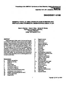
In summary, all data input and output are carried out through the master processor. The most time-consuming computations (assembling the Jacobian matrix, updating thermophysical parameters, solving linear equation systems.) are distributed to all processors involved. The memory requirements are also distributed to all processors. Distributing both computing and memory requirements is essential for solving large-scale problems and obtaining better parallel performance. Figure 3-2 gives an abbreviated overview of the program flow chart.
23
Start All PEs: Declare variables and arrays, but do not allocate array space
PE0: Read input data, not include property data for each block and connection
PE1-PEn: Receive parameters from PE0
PE0: Broadcast parameters to all PEs PE0: Grid partitioning PE0: Set up global DVBR format matrix
PE1-PEn: Receive local part DVBR format matrix from PE0
PE0: Distribute DVBR matrix to all PEs
All PEs: Allocate memory spaces for all arrays for storing the properties of blocks and connections in each PE
PE0: Read data of block and connection properties and distribute the data
PE1-PEn: Receive the part of data which belongs to current PE
All PEs: Exchange external set of data All PEs: set up local equation system at each PE All PEs: Solve the equations using Newton’s method All PEs: Update thermophysical parameters Converged?
no
yes Next time step?
yes
no All PEs: Reduce solutions to PE0 PE0: Output results
End
Figure 3-2. Simplified flow chart of TOUGH2-MP
24
Table 4-1. TOUGH2-MP input data blocks§ Keyword
Function
TITLE One data record (single line) with a title for the simulation problem (first record) VER14
Optional; invoke using the Version 1.4 processing features.
MESHM
Optional; parameters for internal grid generation through MESHMaker
ROCKS
Hydrogeologic parameters for various reservoir domains
MULTI
Optional; specifies number of fluid components and balance equations per gridblock; applicable only for certain fluid property (EOS) modules
START
Optional; one data record for more flexible initialization
PARAM
Computational parameters.
RPCAP
Optional; parameters for relative permeability and capillary pressure functions
TIMES
Optional; specification of times for generating printout
*ELEME
List of gridblocks (volume elements)
*CONNE
List of flow connections between gridblocks
*GENER
Optional; list of mass or heat sinks and sources
INDOM
Optional; list of initial conditions for specific reservoir domains
*INCON
Optional; list of initial conditions for specific gridblocks
NOVER (optional)
Optional; if present, suppresses printout of version numbers and dates of the program units executed in a TOUGH2 run
TIMBC
Optional; introducing a table for time-dependent pressure boundary.
RTSOL
Optional; provide linear solver parameters
FOFT
Optional; list of gridblocks for time-dependent output
GOFT
Optional; list of source/sink gridblocks for time-dependent output.
COFT
Optional; list of connections for time-dependent output
DIFFU
Optional; introduce diffusion coefficients
SELEC
Optional, provide parameters for requirements by specific modules
ENDCY (last record)
One record to close the TOUGH2 input file and initiate the simulation
ENDFI
Alternative to “ENDCY” for closing a TOUGH2 input file; will cause flow simulation to be skipped; useful if only mesh generation is desired
§
Blocks labeled with a star * can be provided as separate disk files, in which case they would be omitted from the INFILE file.
25
4. DESCRIPTION OF INPUT FILES 4.1 Preparation of Input Data Input of TOUGH2-MP is provided through a file named INFILE or separate additional files (e.g. MESH, GENER, INCON), organized into a number of data blocks, labeled by five-character keywords (Table 4-1). The input file “INFILE” of TOUGH2-MP is compatible with the input file for TOUGH2 V1.4 and T2R3D V1.4 (Wu, 1999 and 2000), and also the TOUGH2 V2.0. The parallel program may also receive additional data input through optional input files (See Section 4.4 for details). In general, input files for V1.4 and 2.0 or combination of both are readily acceptable for the parallel simulator.
4.2 Input File Format This section presents the data input formats for TOUGH2-MP. Most formats are identical to corresponding inputs in V1.4 and V2.0. Please refer to the TOUGH2 User’s Guide Version 2.0 (Pruess et al., 1999, Wu et. al., 1996), and User’s Manual for TOUGH2 V1.4 and T2R3D V1.4 (Wu, 1999 and 2000) for more information.
TITLE
is the first record of the input file, containing a header of up to 80 characters, to be printed on the output. This can be used to identify a problem. If no title is desired, leave this record blank.
VER14
the default version of the parallel code is compatible with TOUGH2 V2.0. Some modules (EOS3, EOS9, T2R3D) can be run with both V1.4 or V2.0 (V1.4 has its own specific features). To use V1.4, this keyword must be presented right after the line for TITLE keyword.
MESHM
introduces parameters for internal mesh generation and processing. The MESHMaker input has a modular structure organized by keywords. Detailed instructions for preparing MESHMaker input are given in Section 4.3.
26
Record MESHM.1 Format(A5) WORD WORD
Enter one of several keywords, such as RZ2D, RZ2DL, XYZ, MINC, to generate different kinds of computational meshes.
Record MESHM.2
ENDFI
A blank record closes the MESHM data block.
is a keyword that can be used to close a TOUGH2-MP input file when no flow simulation is desired. This will often be used for a mesh generation run when some hand-editing of the mesh will be needed before the actual flow simulation.
ROCKS
introduces material parameters for different reservoir domains.
Record ROCKS.1 Format (A5, I5, 7E10.4) MAT, NAD, DROK, POR, (PER (I), I = 1,3), CWET, SPHT MAT
Material name (rock type).
NAD
If zero or negative, defaults will take effect for a number of parameters (see below); ≥1: will read another data record to override defaults. ≥2: will read two more records with domain-specific parameters for relative permeability and capillary pressure functions.
DROK
Rock grain density (kg/m3)
POR
Default porosity (void fraction) for all elements belonging to domain "MAT" for which no other porosity has been specified in block INCON. Option "START" is necessary for using default porosity.
PER(I),
I = 1,3 absolute permeabilities along the three principal axes, as specified by ISOT in block CONNE.
27
CWET
Formation heat conductivity under fully liquid-saturated conditions (W/m ˚C).
SPHT
Rock grain specific heat (J/kg ˚C). Domains with SPHT > 104 J/kg ˚C will not be included in global material balances. This provision is useful for boundary nodes, which are given very large volumes so that their thermo-dynamic state remains constant. Because of the large volume, inclusion of such nodes in global material balances would make the balances useless.
Record ROCKS.1.1
(optional, NAD ≥ 1 only)
Format (8E10.4) COM,
EXPAN,
CDRY,
TORTX,
GK,
PERF(1)/XKD3,
PERF(2)/XKD4, PERF(3) COM
Pore compressiblity (Pa-1), (1 φ)(∂φ
EXPAN
Pore expansivity (1/ ˚C), (1 φ)(∂φ ∂T)P (default is 0).
CDRY
Formation heat conductivity under desaturated conditions (W/m
∂P)T
(default is 0).
˚C), (default is CWET). TORTX
Tortuosity factor for binary diffusion.
GK
Klinkenberg parameter b (Pa-1) for enhancing gas phase permeability according to the relationship kgas = kliq * (1 + b/P).
The following three slots are for different parameters in Version 1.4 and 2.0. For Ver 1.4: PERF(1)
Absolute fracture continuum permeabilities along one principal axis, as specified by ISOT=1 in block CONNE, for using the ECM only.
PERF(2)
Absolute fracture continuum permeabilities along one principal axis, as specified by ISOT=2 in block CONNE, for using the ECM only.
PERF(3)
Absolute fracture continuum permeabilities along one principal axis, as specified by ISOT=3 in block CONNE, for using the ECM only.
28
For a dual-continuum model of dual-permeability, double-porosity or MINC, PERF(3) is effective porosity of fracture continuum and in this case, PERF(1) and PERF(2) must be set to zero. For Ver 2.0: XKD3
Distribution coefficient for parent radionuclide, Component 3, in the aqueous phase, m3/kg (EOS7R only).
XKD4
Distribution coefficient for daughter radionuclide, Component 4, in the aqueous phase, m3/kg (EOS7R only).
Record ROCKS.1.2
(optional, NAD ≥ 2 only)
Format (I5, 5X,7E10.4) IRP, (RP(I), I= 1,7) IRP
Integer parameter to choose type of relative permeability function (see Appendix B).
RP(I), I = 1, ..., 7 parameters for relative permeability function (Appendix B). Record ROCKS.1.3
(optional, NAD ≥ 2 only)
Format (I5, 5X,7E10.4) ICP, (CP(I), I = 1,7) ICP
Integer parameter to choose type of capillary pressure function (see Appendix B).
CP(I)
I = 1, ..., 7 parameters for capillary pressure function (Appendix C). Repeat records 1, 1.1, 1.2, and 1.3 for any number of reservoir domains.
For T2R3D, an additional rock card is needed for radionuclide transport properties, which should be located right before the ROCKS.1.2 Record ROCKS.1.1.5 (For T2R3D only) FORMAT(6E10.4) ALPHAL, ALPHAT, ALAMDA, SKD, DIFFM, ALPHAFM ALPHAL
longitudinal dispersivity (m)
ALPHAT
transverse dispersivity (m)
ALAMDA
radioactive decay constant = ln(2)/t1/2 (1/s)
29
SKD
distribution coefficient, Kd (m3/kg)
DIFFM
molecular diffusion coefficient in liquid phase (m2/s)
ALPHAFM
averaged dispersivity for fracture/matrix (m)
Record ROCKS.2
MULTI
A blank record closes the ROCKS data block.
Permits the user to select the number and nature of balance equations that will be solved. The keyword MULTI is followed by a single data record. For most EOS modules this data block is not needed, as default values are provided internally. Available parameter choices are different for different EOS modules.
Record MULTI. l Format (5I5) NK, NEQ, NPH, NB, NKIN NK
Number of mass components.
NEQ
number of balance equations per grid block. Usually we have NEQ =NK + 1, for solving NK mass and one energy balance equation. Some EOS modules allow the option NEQ = NK, in which case only NK mass balances and no energy equation will be solved.
NPH
Number of phases that can be present (2 for mostt modules).
NB
Number of secondary parameters in the PAR-array (see Fig. 3) other than component mass fractions. Available options include NB = 6 (no diffusion) and NB = 8 (include diffusion). It always equal 8 for Ver 1.4.
NKIN
Number of mass components in INCON data (default is NKIN = NK). This parameter can be used, for example, to initialize an EOS7R simulation (NK= 4 or 5) from data generated by EOS7 (NK = 2 or 3). If a value other than the default is to be used, then data block MULTI must appear before any initial conditions in data blocks PARAM, INDOM, or INCON.
30
START
(optional) A record with START typed in columns 1-5 allows a more flexible initialization. More specifically, when START is present, INCON data can be in arbitrary order, and need not be present for all gridblocks (in which case defaults will be used). Without START, there must be a one-to-one correspondence between the data in blocks ELEME and INCON.
PARAM
introduces computation parameters, time stepping information, and default initial conditions.
Record PARAM.1 Format (2I2, 3I4, 24I1, 10X, 2E10.4, I10). NOITE, KDATA, MCYC, MSEC, MCYPR, (MOP(I), I = 1, 24), TEXP, BE, MCYCF, MOP(25) NOITE
Specifies the maximum number of Newtonian iterations per time step (default is 8)
KDATA
Specifies amount of printout (default is 1). = 0 or 1: print a selection of the most important variables. = 2: in addition, print mass and heat fluxes and flow velocities. = 3: in addition, print primary variables and their changes.
MCYC
Maximum number of time steps to be calculated.
MSEC
Maximum duration, in CPU seconds, of the simulation (default is infinite).
MCYPR
Printout will occur for every multiple of MCYPR steps (default is 1).
MOP(I), I = 1,24 allows choice of various options, which are documented in printed output from a TOUGH2 run. MOP(1)
If unequal 0, a short printout for nonconvergent iterations will be generated. MOP(2) through MOP(6) generate additional printout in various subroutines, if set unequal 0. This feature should not be needed in
31
normal applications, but it will be convenient when a user suspects a bug and wishes to examine the inner workings of the code. The amount of printout increases with MOP(I) (consult source code listings for details). MOP(2)
CYCIT (main subroutine).
MOP(3)
MULTI (flow and accumulation terms).
MOP(4)
QU (sinks/sources).
MOP(5)
EOS (equation of state).
MOP(6)
LINEQ (linear equations).
MOP(7)
If unequal 0, a printout of input data will be provided. Calculation option choices are as follows:
MOP(9)
Determines the composition of produced fluid with the MASS option (see GENER, below). The relative amounts of phases are determined as follows: = 0:
according to relative mobility in the source element.
= 1:
produced source fluid has the same phase composition as
the producing element. MOP(10)
Chooses the interpolation formula for heat conductivity of rock as a function of liquid saturation (Sl)
MOP(11)
= 0:
C(Sl) = CDRY + SQRT(Sl* [CWET - CDRY])
= 1:
C(Sl) = CDRY + Sl * (CWET - CDRY)
= 2:
C = C0+C1*T+C2*Sl+C3*POR.
Determines evaluation of mobility and permeability at interfaces. = 0:
mobilities are upstream weighted with WUP (see PARAM.3), permeability is upstream weighted.
= 1:
mobilities are averaged between adjacent elements, permeability is upstream weighted.
= 2:
mobilities are upstream weighted, permeability is harmonic weighted.
= 3:
mobilities are averaged between adjacent elements, permeability is harmonic weighted.
32
= 4: MOP(12)
mobility and permeability are both harmonic weighted.
Determines interpolation procedure for time dependent sink/source data (flow rates and enthalpies). = 0:
triple linear interpolation; tabular data are used to obtain interpolated rates and enthalpies for the beginning and end of the time step; the average of these values is then used.
= 1:
step function option; rates and enthalpies are taken as averages of the table values corresponding to the beginning and end of the time step.
=2:
rigorous step rate capability for time dependent generation data. A set of times ti and generation rates qi provided in data block GENER is interpreted to mean that sink/source rates are piecewise constant and change in discontinuous fashion at table points.
MOP(14)
MOP(15)
Specifies if 5- or 8-character elements are used in the mesh. = 0:
5-character elements are used.
= 1:
8-character elements are used.
Determines conductive heat exchange with impermeable confining layers = 0:
heat exchange is off.
= 1:
heat exchange is on (for gridblocks that have a non-zero heat transfer area; see data block ELEME). This option has not been implemented in TOUGH2-MP.
MOP(16)
Provides automatic time step control. Time step size will be increased if convergence occurs within ITER ≤ MOP(16) NewtonRaphson iterations. It is recommended to set MOP(16) in the range of 2 - 4.
MOP(17)
Specifies generation of a flow9.dat file for T2R3D transport simulations (EOS9 only). = 0:
no.
= 1:
yes.
33
MOP(18)
Selects handling of interface density. = 0:
perform upstream weighting for interface density.
> 0:
average interface density between the two gridblocks. However, when one of the two phase saturations is zero, upstream weighting will be performed.
MOP(19)
Switch used by different EOS modules for conversion of primary variables.
MOP(20)
MOP(21)
MOP(24)
Allows for different formats of CONNE and GENER indexes. = 0:
use format (16I5).
= 1:
use format (10I8)
Allows for one more N/R iteration after solution. = 0:
no need for one more iteration.
= 1:
perform one more iteration after convergence.
Determines handling of multiphase diffusive fluxes at interfaces. =0:
harmonic weighting of fully coupled effective multiphase diffusivity.
=1:
separate harmonic weighting of gas and liquid phase diffusivities.
TEXP
Parameter for temperature dependence of gas phase diffusion coefficient.
BE
(Optional) parameter for effective strength of enhanced vapor diffusion; if set to a non-zero value, will replace the parameter group φτ0τβ for vapor diffusion.
MCYCF
Allows for more time steps to be run for each simulation by MCYC = MCYCF, if MCYCF > MCYC.
Record PARAM.2 Format (4E10.4, A5, 5X,3E10.4) TSTART, TIMAX, DELTEN, DELTMX, ELST, GF, REDLT, SCALE TSTART
Starting time of simulation in seconds (default is 0).
34
TIMAX
Time in seconds at which simulation should stop (default is infinite).
DELTEN
Length of time steps in seconds. If DELTEN is a negative integer, DELTEN = -NDLT, the program will proceed to read NDLT records with time step information. Note that -NDLT must be provided as a floating point number, with decimal point.
DELTMX
Upper limit for time step size in seconds (default is infinite)
ELST
Writes a file for time versus primary variables for selected elements at all the times, when ELST = RICKA (Same as the function with keyword FOFT).
GF
Magnitude (m/sec2) of the gravitational acceleration vector. Blank or zero gives "no gravity" calculation.
REDLT
Factor by which time step is reduced in case of convergence failure or other problems (default is 4). If REDLT1) for which time versus primary variables is printed at each time step into files: FOFT_P.xxx. The file extension xxx is the identification number of the processor at which the output was generated.
Record ROCKS.2.1.2, 2.1.3, etc
(optional, ELST = RICKA only) Number of
records = NELIST Format (A5) for MOP(14) = 0 or Format (A8) for MOP(14) = 1. EPLIST(I) EPLIST(I),
I = 1,2, …, NELIST, element’s names for which time versus primary variables needs to be printed at each time step into files: FOFT_P.xxx.
35
Record PARAM.2.2.1, 2.2.2, etc. Format (8E10.4) (DLT(I), I = 1, 100) DLT(I)
Length (in seconds) of time step I. This set of records is optional for DELTEN = - NDLT, a negative integer. Up to 13 records can be read, each containing 8 time step data. If the number of simulated time steps exceeds the number of DLT(I), the simulation will continue with time steps equal to the last non-zero DLT(I) encountered. When automatic time step control is chosen (MOP(16) > 0), time steps following the last DLT(I) input by the user will increase according to the convergence rate of the Newton-Raphson iteration. Automatic time step reduction will occur if the maximum number of NewtonRaphson iterations is exceeded (parameter NOITE, record PARAM.1)
Record PARAM.3 Format (6E10.4) RE1, RE2, U, WUP, WNR, DFAC RE1
Convergence criterion for relative error (default= 10-5).
RE2
Convergence criterion for absolute error, see (default= 1).
U
Not be used
WUP
Upstream weighting factor for mobilities and enthalpies at interfaces (default = 1.0 is recommended). 0 ≤ WUP ≤ 1.
WNR
Weighting factor for increments in Newton/Raphson - iteration (default = 1.0 is recommended). 0 < WNR ≤ 1.
DFAC
Increment factor for numerically computing derivatives (default value is DFAC = 10
- k/2,
where k, evaluated internally, is
the number of significant digits of the floating point processor used; for 64-bit arithmetic, DFAC ≈ 10-8).
36
Record PARAM.4
Introduces a set of primary variables which are used as default initial conditions for all gridblocks that are not assigned by means of data blocks INDOM or INCON. Option START is necessary to use default INCON. Format (4E20.14) DEP(I), I = 1, NK+1
The number of primary variables, NK+1, is normally assigned internally in the EOS module, and is usually equal to the number NEQ of equations solved per gridblock. See data block MULTI for special assignments of NK. Different sets of primary variables are in use for different EOS modules.
INDOM
introduces domain-specific initial conditions. These will supersede default initial conditions specified in PARAM.4, and can be overwritten by element-specific initial conditions in data block INCON. Option START is needed to use INDOM conditions.
Record INDOM. l Format(A5) MAT MAT
Name of a reservoir domain, as specified in data block ROCKS.
Record INDOM.2 Format(4E20.13) Xl, X2, X3, …… A set of primary variables assigned to all gridblocks in the domain specified in record INDOM. l. Different sets of primary variables are used for different EOS modules. Record INDOM.3
37
A blank record closes the INDOM data block. Repeat records INDOM. l and INDOM.2 for as many domains as desired. The ordering is arbitrary and need not be the same as in block ROCKS.
INCON
introduces element-specific initial conditions.
Record INCON.1 For MOP(14) = 0, 5-character element Format (A3, I2, 2I5,E15.9) EL, NE, NSEQ, NADD, PORX For MOP(14) = 1, 8 character element Format (A6, I2) EL, NE EL, NE
Code name of element.
NSEQ
Number of additional elements with the same initial conditions (used only for 5-character element name).
NADD
Increment between the code numbers of two successive elements with identical initial conditions (used only for 5-character element name).
PORX
Porosity; if zero or blank, porosity will be taken as specified in block ROCKS if option START is used.
Record INCON.2
specifies primary variables.
Format (4E20.14) Xl, X2, X3, X4 A set of primary variables for the element specified in record INCON.l. INCON specifications will supersede default conditions specified in PARAM.4, and domain-specific conditions that may have been specified in data block INDOM. Different sets of primary variables are used for different EOS modules. Record INCON.3
A blank record closes the INCON data block. Alternatively, initial condition information may terminate on a record with “+++” typed in the first three columns, followed by
38
time stepping information. This feature is used for a continuation run from a previous TOUGH2-MP simulation.
NOVER (optional) One record with NOVER typed in columns 1-5 will suppress printing of a summary of versions and dates of the program units used in a TOUGH2-MP run.
SELEC
(optional) introduces a number of integer and floating point parameters that are used for different purposes in different TOUGH2 modules.
Record SELEC.1 Format(16I5) IE(I), I=1,16 IE(1)
number of records with floating point numbers that will be read (default is IE(1) = 1; maximum values is 64).
Record SELEC.2, SELEC.3, ..., SELEC.IE(1)*8 Format(8E10.4) FE(I), I=1,IE(1)*8 Provide as many records with floating point numbers as specified in IE(1), up to a maximum of 64 records.
RPCAP
introduces information on relative permeability and capillary pressure functions, which will be applied for all flow domains for which no data were
specified
in
records
ROCKS.1.2
and
ROCKS.1.3. A catalog of relative permeability and capillary pressure functions is presented in Appendix B and Appendix C, respectively. Record RPCAP.1 Format (I5,5X,7E10.4) IRP, (RP(I),I = 1, 7)
39
IRP
Integer parameter to choose type of relative permeability function (see Appendix B).
RP(I), I = 1, ..., 7 parameters for relative permeability function (Appendix B). Record RPCAP.2 Format (I5,5X,7E10.4) ICP, (CP(I), I = 1, 7) ICP
Integer parameter to choose type of capillary pressure function (see Appendix C).
CP(I)
I = 1, ..., 7 parameters for capillary pressure function (Appendix C).
TIMES
permits the user to obtain printout at specified times (optional). This printout will occur in addition to printout specified in record PARAM.1.
Record TIMES.1 Format (2I5,2E10.4) ITI, ITE, DELAF, TINTER ITI
Number of times provided on records TIMES.2, TIMES.3, etc., (see below; restriction: ITI ≤ 100).
ITE
Total number of times desired (ITI ≤ ITE ≤ 100; default is ITE = I TI).
DELAF
Maximum time step size after any of the prescribed times have been reached (default is infinite).
TINTER
Time increment for times with index ITI, ITI+1, ..., ITE.
Record TIMES.2, TIMES.3, etc. Format (8E10.4) (TIS(I), I = l, ITI) TIS(I)
List of times (in ascending order) at which printout is desired.
40
ELEME
introduces element (gridblock) information. See Section 4.4 for additional explanations.
Record ELEME.1 For MOP(14) = 0, 5-character element Format (A3, I2, 2I5, A3, A2, 6E10.4) EL, NE, NSEQ, NADD, MA1, MA2, VOLX, AHTX, PMX, X, Y, Z For MOP(14) = 1, 8-character element Format (A6, I2, 7X, A3, A2, 6E10.4) EL, NE, MA1, MA2, VOLX, AHTX, PMX, X, Y, Z EL, NE
Five-character (or eight-character with MOP(14) = 1) code name of an element. The first three or six characters are arbitrary; the last two characters must be numbers.
NSEQ
Number of additional elements having the same volume and belonging to the same reservoir domain (Only for MOP(14) = 0 ).
NADD
Increment between the code numbers of two successive elements. (Only for MOP(14) = 0)
MA1, MA2
A five-character material identifier corresponding to one of the reservoir domains as specified in block ROCKS. If the first three characters are blanks and the last two characters are numbers then they indicate the sequence number of the domain as entered in ROCKS. If both MA1 and MA2 are left blank the element is by default assigned to the first domain in block ROCKS.
VOLX
Element volume (m3).
AHTX
Interface area (m2) for heat exchange with semi-infinite confining beds.
PMX
permeability modifier (optional, active only when a domain ‘SEED’ has been specified in the ROCKS block; see TOUGH2 V2 User’s Guide). It will be used as multiplicative factor for the permeability parameters from block ROCKS. Simultaneously,
41
strength of capillary pressure will be scaled as 1/SQRT(PMX). PMX = 0 will result in an impermeable block. Random permeability modifiers can be generated internally, see detailed comments in the TOUGH2-MP output file. The PMX may be used to specify spatially correlated heterogeneous fields, but users need their own preprocessing programs for this, as TOUGH2 provides no internal capabilities for generating such fields. X, Y, Z
Cartesian coordinates of gridblock centers. These may be included in the ELEME data to make subsequent plotting of results more convenient. The coordinate data are not used internally by TOUGH2-MP, except with EOS9 for initialization of a gravitycapillary equilibrium.
Repeat record ELEME.1 for the number of elements desired. Record ELEME.2
CONNE
A blank record closes the ELEME data block.
introduces information for the connections (interfaces) between elements. See Section 4.4 for additional explanations.
Record CONNE.1 For MOP(14) = 0, 5-character element Format (A3, I2, A3, I2, 4I5, 5E10.4) EL1, NE1, EL2, NE2, NSEQ, NAD1, NAD2, ISOT, D1, D2, AREAX, BETAX, SIGX/IFM_CON For MOP(14) = 1, 8-character element Format (A6, I2, A6, I2, 9X, I5, 5E10.4) EL1, NE1, EL2, NE2, ISOT, D1, D2, AREAX, BETAX, SIGX/IFM_CON EL1, NE1
Code name of the first element.
EL2, NE2
Code name of the second element.
NSEQ
Number of additional connections in the sequence (for MOP(14)=0 only).
42
NAD1
Increment of the code number of the first element between two successive connections (for MOP(14)=0 only).
NAD2
Increment of the code number of the second element between two successive connections (for MOP(14)=0 only).
ISOT
Set equal to 1, 2, or 3; specifies absolute permeability to be PER(ISOT) for the materials in elements (EL1, NE1) and (EL2, NE2), where PER is read in block ROCKS. This allows assignment of different permeabilities, e.g., in the horizontal and vertical direction.
Note that in this version, several schemes of fracture-matrix (F-M) interface area reduction for F-M local connection and mobility weighting are implemented using ISOT, which is set to a negative integer as follows:
= -1
F-M interconnection area used for calculating flow of a fluid is multiplied by the upstream saturation of the fluid,
= -2
mobility of the lower absolute permeability block is used for flow calculation along this connection.
= -3
F-M interconnection area for calculating flow of a fluid is multiplied by a constant factor ( = RP(7) from fracture rock material) and by the upstream relative permeability to the fluid. This scheme is called weeps type model.
= -4
F-M interconnection area for calculating flow of a fluid is multiplied by the upstream relative permeability to the fluid,
= -9
F-M interconnection area for calculating flow of a fluid is multiplied by a constant factor ( = RP(6) from fracture rock material),
= -10 F-M interconnection area for calculating flow of the liquid is modified by the active fracture model (Liu et al., 1998).
43
D1
Distance (m) from first element to common interface.
D2
Distance (m) from second element to common interface.
AREAX
Interface area (m2).
BETAX
Cosine of the angle between the gravitational acceleration vector and the line between the two elements. GF * BETAX > 0 ( 1 only).
GX
Constant generation rate; positive for injection, negative for production; GX is mass rate (kg/sec) for generation types COMl, COM2. COM3, etc., and MASS; it is energy rate (J/s) for a HEAT sink/source. For wells on deliverability, GX is productivity index PI (m3).
EX
Fixed specific enthalpy (J/kg) of the fluid for mass injection (GX>0). For wells on deliverability against fixed bottomhole
46
pressure, EX is bottomhole pressure Pwb (Pa), at the center of the topmost producing layer in which the well is open. HX
Tickness of layer (m; wells on deliverability with specified bottomhole pressure only).
Record GENER.l.l (optional, LTAB > l only) Format (4E14.7) Fl(L), L=l, LTAB F1
Generation times
Record GENER.1.2 (optional, LTAB > 1 only) Format (4E14.7) F2(L), L=1, LTAB F2
Generation rates.
Record GENER.1.3 (optional, LTAB > 1 and ITAB non-blank only) Format (4E14.7) F3(L), L=1, LTAB F3
Specific enthalpy of produced or injected fluid. Repeat records GENER.1, 1.1, 1.2, and 1.3 for the number of sinks/sources desired.
Record GENER.2
A blank record closes the GENER data block.
Alternatively, generation information may terminate on a record with ‘+++’ typed in the first three columns, followed by element cross-referencing information.
DIFFUSION (optional; needed only for NB≥8, for Ver 2.0 only) introduces diffusion coefficients. Record DIFFU.1 Format(8E10.4) FDDIAG(I,1), I=1,NPH diffusion coefficients for mass component # 1 in all phases (I=1: gas; I=2: aqueous; etc.) Record DIFFU.2
47
Format(8E10.4) FDDIAG(I,2), I=1,NPH diffusion coefficients for mass component # 2 in all phases (I=1: gas; I=2: aqueous; etc.) Provide a total of NK records with diffusion coefficients for all NK mass components. See Pruess et al. (1999) for additional parameter specifications for diffusion.
FOFT
(optional) introduces a list of elements (grid blocks) for which time dependent data are to be written out for plotting to a file called FOFT_P.xxx during the simulation. The file extension xxx is the identification number of the processor at which the output was generated.
Record FOFT.1 Format(A5) (for MOP(14)=0) Format(A8) (for MOP(14)=1) EOFT(I)
EOFT is an element name. Repeat for up to 100 elements, one per record. Record FOFT.2 A blank record closes the FOFT data block.
COFT
(optional) introduces a list of connections for which timedependent data are to be written out for plotting to file FOFT_P.xxx during the simulation.
Record COFT.1 Format(A10) (for MOP(14)=0) Format(A16) (for MOP(14)=1) ECOFT(I)
48
ECOFT is a connection name, i.e., an ordered pair of two element names. Repeat for up to 100 connections, one per record.
Record COFT.2 A blank record closes the COFT data block.
(optional) introduces a list of sinks/sources for which time-
GOFT
dependent data are to be written out for plotting to file FOFT_P.xxx during the simulation. Record GOFT.1 Format(A5) (for MOP(14)=0) Format(A8) (for MOP(14)=1) EGOFT(I)
EGOFT is the name of an element in which a sink/source is defined. Repeat for up to 100 sinks/sources, one per record. When no sinks or sources are specified here, by default tabulation will be made for all.
Record GOFT.2 A blank record closes the GOFT data block.
TIMBC
(optional) introduces a table (external data file, named as “timvsp.dat”, must be located at the simulation working directory) for time-dependent pressure boundary conditions.
File “timevsp.dat” format: FORMAT(2I5) NPOINT, NTPTAB (number of time points and gridblocks at which pressure boundary conditions will be specified)
FORMAT(4E14.7)
49
TIMBCV(I), I=1, NPOINT (times for each time point)
FORMAT(A5)
for
MOP(14)=0,
and
FORMAT(A8)
for
MOP(14)=1 BCELEM(I), I=1, NTPTAB (name list of the NTPRAB gridblocks)
FORMAT(4E14.7) PGBCEL(I,J), I=1, NPOINT; J=1,NTPTAB (boundary pressure provided at the NPONIT time points for all the
NTPTAB
gridblocks
RTSOL
(optional) introduces additional time stepping, iteration and solver parameters. This keyword inherits from VER 1.4. Most parameters under this keyword have not been used in TOUGH2-MP.
Record RTSOL.1 Format (2E10.3, 6I5) PREC, RTOL, INFO, IPLVL, NITMX, NORT, KACCEL, IREDB All these parameters have not been used in this version. Record RTSOL.2 Format (7F10.3,I5) DTMIN, DTMAX, DSTNOM, DXTMAX,TMULFC, RELXSN, RELXXN, ICOLEY DTMIN
minimum time step size in seconds.
DSTNOM
maximum allowable saturation change per time step (default=0.2).
TMULFC
Time step size increasing rate when Newton iteration converges in less then MOP(16) iterations, see also REDLT.
ICOLEY
flag for evaluating an underrelaxation factor for updating primary variables over Newton iteration; = 0: if no underrelaxation scheme is used, = 1: if Cooley underrelaxation scheme is used, and
50
= 2: if an underrelaxation scheme is determined using DSTNOM, normalized maximum changes in saturation. Other parameters have not been used in this version.
ENDCY
closes the TOUGH2 input file and initiates the simulation.
Note on closure of blocks CONNE, GENER, and INCON The conventional way to indicate the end of any of the above data blocks is by means of a blank record. There is an alternative available if the user constructs an input file from files MESH, GENER, or SAVE, which have been generated by a previous TOUGH2 or TOUGH2-MP run. These files are written exactly according to the specifications of data blocks ELEME and CONNE (file MESH), GENER (file GENER), and INCON (file SAVE), except that the CONNE, GENER, and INCON data terminate on a record with “+++” in Columns 1-3, followed by some cross-referencing (indexing) and restart information. TOUGH2-MP will accept this type of input, and in this case there is no blank record at the end of an indicated data block. The cross-referencing information will not be read by the parallel code, because this information may be not correct when the model has a total of more than 100,000 gridblocks. The parallel code uses a very efficient index searching algorithm that computes the connection and gridblock indices at the beginning of every simulation run.
4.3 Input Formats for MESHMAKER The MESHMaker module performs internal mesh generation and processing. This module has not been parallelized and is run on the master processor only. In general, the input and output of MESHMaker for TOUGH2-MP are identical to V2.0, except that the parallel version allows generating multi-million gridblocks for Cartesian X-Y-Z mesh. The input for MESHMaker has a modular structure and a variable number of records; it begins with keyword MESHM and ends with a blank record.
There are three submodules available in MESHMaker: keywords RZ2D or RZ2DL invoke generation of a one or two-dimensional radially symmetric R-Z mesh; XYZ
51
initiates generation of a one, two, or three-dimensional Cartesian X-Y-Z mesh; and MINC calls a modified version of the GMINC program (Pruess, 1983) to subpartition a primary porous medium mesh into a secondary mesh for fractured media, using the method of “multiple interacting continua” (Pruess and Narasimhan, 1985). The meshes generated under keyword RZ2D or XYZ are internally written to file MESH. The MINC processing operates on the data in file MESH, so that invoking the RZ2D or XYZ options, or assignment of ELEME and CONNE blocks in the INPUT file, must precede the MESHMaker/MINC data. We shall now separately describe the preparation of input data for the three MESHMaker submodules. 4.3.1 Generation of Radially Symmetric Grids Keyword RZ2D (or RZ2DL) invokes generation of a radially symmetric mesh. Values for the radii to which the gridblocks extend can be provided by the user or can be generated internally (see below). Nodal points will be placed half-way between neighboring radial interfaces. When RZ2D is specified, the mesh will be generated by columns; i.e., in the ELEME block, we will first have the gridblocks at smallest radius for all layers, then the next largest radius for all layers, and so on. With keyword RZ2DL, the mesh will be generated by layers; i.e., in the ELEME block, we will first have all gridblocks for the first (top) layer from smallest to largest radius, then all gridblocks for the second layer, and so on. Apart from the different ordering of elements, the two meshes for RZ2D and RZ2DL are identical. Assignment of inactive elements would be made by using a text editor on the RZ2D-generated MESH file, and moving groups of elements towards the end of the ELEME block, past a dummy element with zero volume. RZ2D makes it easy to declare a vertical column inactive, facilitating assignment of boundary conditions in the vertical, such as a gravitationally equilibrated pressure gradient. RZ2DL, on the other hand, facilitates implementation of areal (top and bottom layer) boundary conditions.
52
RADII
is the first keyword following RZ2D; it introduces data for defining a set of interfaces (gridblock boundaries) in the radial direction.
Record RADII.l Format(I5) NRAD NRAD
Number of radius data that will be read. At least one radius must be provided, indicating the inner boundary of the mesh.
Record RADII.2, RADII.3, etc. Format(8E10.4) RC(I), I = 1, NRAD RC(I)
A set of radii in ascending order.
EQUIDistant introduces data on a set of equal radial increments. Record EQUID. l Format(I5, 5X, E10.4) NEQU, DR NEQU
Number of desired radial increments.
DR
Magnitude of radial increment.
Note: At least one radius must have been defined via block RADII before EQUID can be invoked.
LOGARithmic introduces data on radial increments that increase from one to the next by the same factor (∆Rn+l = f • ∆Rn). Record LOGAR. l Format(A5, 5X, 2E10.4) NLOG, RLOG, DR NLOG
number of additional interface radii desired.
RLOG
Desired radius of the last (largest) of these radii.
53
DR reference radial increment: the first ∆R generated will be equal to f • DR, with f internally determined such that the last increment will bring total radius to RLOG. f0, the code will not perform domain partitioning and partition data will be read directly from file “part.dat” at the working directory. Default PartReady=0.
The default values of MNEL and NCON are 500,000 and 2,300,000. The two parameters are required only in generating MESHA and MESHB and when a model has more than 500,000 gridblocks or 2,300,000 connections.
From the second line and below, each line provides a parameter. These parameters give options or parameters for running the Aztec and METIS packages, and SAVE file output frequency control. The parameters can be in any order. If one parameter is not present, its default value will be used. Each line in the file consists of two terms. The first term is parameter’s name and the second term is its value. Detailed content of the parameters is discussed below.
AZ_solver AZ_cg
Specifies solution algorithm, available solvers: conjugate gradient (only applicable to symmetric positive definite matrices).
AZ_gmres
restarted generalized minimal residual.
AZ_cgs
conjugate gradient squared.
AZ_tfqmr
transpose-free quasi-minimal residual.
AZ_bicgstab
bi-conjugate gradient with stabilization.
AZ_lu
sparse direct solver (single processor only).
AZ_scaling
Specifies scaling algorithm, user can select from:
AZ_none
no scaling.
AZ_Jacobi
point Jacobi scaling.
AZ_BJacobi
Block Jacobi scaling where the block size corresponds to the
63
VBR blocks. Az_row_sum
scale each row so the magnitude of its elements sum to 1.
AZ_sym_diag
symmetric scaling so diagonal elements are 1.
AZ_sym_row_sum symmetric scaling using the matrix row sums. AZ_precond
Specifies preconditioner. Available selections include:
AZ_none
no preconditioning.
AZ_Jacobi
k step Jacobi (or block Jacobi for DVBR matrices)
AZ_Neumann
Neumann series polynomial.
AZ_ls
least-squares polynomial.
AZ_sym_GS
non-overlapping domain decomposition (additive Schwarz) k step symmetric Gauss-Seidel.
AZ_dom_decomp AZ_tol
domain decomposition preconditioner (additive Schwarz).
Specifies tolerance value used in conjunction with convergence tests.
AZ_type_overlap
Determines how overlapping subdomain results are combined when different processors have computed different values for the same unknown.
AZ_standard
the resulting value of an unknown is determined by the processor owning that unknown.
AZ_symmetric
average the results obtained from different processors corresponding to the same unknown.
AZ_overlap
Determines the submatrices factored with the domain decomposition algorithms.
AZ_max_iter
Maximum number of iterations.
AZ_conv
Determines the residual expression used in convergence check and printing. Available selections include: AZ_r0, AZ_rhs, AZ_Anorm, AZ_noscaled, AZ_sol, AZ_weighted.
AZ_subdomain_solve
Specifies the solver to use on each subdomain when AZ_precond is set to AZ_dom_decomp, available selections include: AZ_lu, AZ_ilut, AZ_ilu, AZ_rilu, AZ_bilu, and AZ_icc.
AZ_reorder
Determines whether RCM reordering will be done in conjunction with domain decomposition incomplete factorizations, 1 yes; 0 no.
64
AZ_pre_calc
Indicates whether to use factorization information from previous calls to AZ_solve, three selections: AZ_calc, AZ_recalc, and AZ_reuse.
AZ_output
Specifies information to be printed, available selections: AZ_all, AZ_none, AZ_warnings, AZ_last, and >0.
EE_partitioner
Specifies the partitioner to be used, user can select partitioners from:
METIS_Kway
uses the multilevel k-way partitioning algorithm. The objective of this partitioning method is to minimize the edgecut. It should be used to partition a graph into a large number of partitions (greater than 8).
METIS_Vkway
uses the multilevel k-way partitioning algorithm. The objective of this partitioning method is to minimize the total communication volume.
METIS_Recursive
uses multilevel recursive bisection. The objective of this partitioning method is to minimize the edgecut, this function should be used to partition a graph into a small number of partitions (less than 8).
EE_output
Output control for solution results. The SAVE file will be written every EE_output time steps. If EE_output=0, no SAVE file will be written out until last time step. A special value of 666888 for this parameter will evoke debugging run, which will produce more informative output.
More options or parameters for the Aztec parallel linear equation solver can be specified. For further discussion, readers may refer to Tuminaro et al. (1999). Table 4-2 presents the default values used in TOUGH2-MP.
65
Table 4-2. Default values of the options and parameters Parameters or options
Values
AZ_solver
AZ_bicgstab
AZ_scaling
AZ_Bjacobi
AZ_pecond
AZ_dom_decomp
AZ_tol
1x10⁻⁶
AZ_type_overlap
AZ_standard
AZ_max_iter
500
AZ_conv
AZ_r0
AZ_subdomain_solve
AZ_ilut
AZ_reorder
1
AZ_pre_calc
AZ_calc
AZ_output
AZ_none
EE_partitioner
METIS_Kway
EE_output
200
INCON During initialization of a TOUGH2 run, all gridblocks are first assigned to the default thermodynamic conditions specified in data block PARAM in file INFILE. The default initial conditions may be superseded by thermodynamic conditions assigned to individual gridblocks in disk file INCON. File format of INCON is the same as in the serial version of the TOUGH2 code.
The INCON file is set up either by user or generated by a previous TOUGH2 run through an output file SAVE (compatible with formats of file or data block INCON for initializing a continuation run). The INCON file can be obtained by simply renaming SAVE file to INCON. If INCON file is set up by the user, only a fraction of the grid blocks may be specified or the blocks may be in a random sequence. Accordingly, TOUGH2-MP will perform a gridblock index search first.
66
GENER The format of file GENER is the same as the block format described in Section 4.2.
part.dat If parameter PartReady in “PARAL.prm” has a value larger than 0, the parallel code will read file “part.dat” from working directory during run-time. The file contains domainpartitioning results. It is read by the following code: open (unit=50,file='part.dat',form='formatted',status='old') read(50,133) nparts,edgecut,NEL read(50,144) (part(iI),iI=1,NEL) 133 format(3I10) 144 format(10I8)
where nparts
Number of portions that the domain has been partitioned into. It must equal to the number of processors/processes used for solving the problem.
edgecut
Number of cut edges.
nel
Total number of elements or gridblocks in the domain.
part
Partitioning result of each gridblock. The integer value indicates that the gridblock is in which processor.
File “part.dat” can be created through a preprocessing program based on user’s special requirements, e.g. based on physical boundaries of modeling domain for grid partitioning.
flow9.dat, flow9b.dat File flow9.dat is required only by the T2R3D module. When running T2R3D for a tracer or contaminant transport simulation, the file, flow9.dat, will provide flow field information. This file is generated by flow simulation (EOS9 module) with option mop(17)=1. File flow9b.dat is an intermediate file which is created by TOUGH2-MP at its first run. The file is in binary format with the same contents as flow9.dat. If flow9b.dat
67
exists in the working directory, the code will ignore the flow9.dat file and read information directly from flow9b.dat. Once the flow9.dat is changed, flow9b.dat must be deleted from the working folder to make the changes take effect. The purpose of using an intermediate file flow9b.dat is to reduce the memory requirement for the master processor and to enhance I/O efficiency.
File flow9b.dat is saved in the following sequence:
write(40) NEL, NCON write(40) (presl(iI),iI=1,NEL) write(40) (satl(iI),iI=1,NEL) write(40) (densl(iI),iI=1,NEL) write(40) (phi(iI),iI=1,NEL) write(40) (FLO(iI),iI=1,NCON) write(40) (vel(iI),iI=1,NCON)
where NEL
Total gridblock number.
NCON
Total connection number.
presl
Liquid pressure
satl
Saturation
densl
Liquid density
phi
Porosity
FLO
Mass flux
vel
Darcy velocity
4.5 Output from TOUGH2-MP TOUGH2-MP produces a variety of output, most of which can be controlled by the user. Information written in the initialization phase on to the standard output file includes parameter settings in the main program for dimensioning of problem-size dependent
68
arrays, and disk files in use. This is followed by documentation on settings of the MOPparameters for choosing program options, and on the EOS-module. During execution, the parallel program can optionally generate a brief message for Newtonian iterations and time steps. At the end, a summary of subroutines used and parallel computation information are provided. In TOUGH2-MP, standard output at user-specified simulation times or time steps is generated by a subroutine called FINALOUT, which is applied to replace the OUT subroutine in TOUGH2 V1.4/V2.0. Each EOS module comes with its own routine FINALOUT. The output file for TOUGH2 is replaced by two files in TOUGH2-MP, named OUTPUT and OUTPUT_DATA. The first file provides problem initialization, time-stepping, and parallel computing information, and the second file gives a complete element-by-element and/or connection-by-connection report of thermodynamic state variables and other important parameters. The sequence for outputs of gridblocks and connections is not in the original sequence as listed in MESH file. It is written out processor-by-processor depending on the domain partition results.
In
addition, there are some minor differences in naming conventions used by different EOS modules.
69
EEE Number of processors = 12 EEE Time perform model computaion = 197230.321027040 EEE of which spent in lin. solv. = 185108.194600105 EEE and spent on other = 12122.1264269352 EEE EEE Total number of time steps = 20000 EEE Average time in Aztec per time step = 9.25540973000526 EEE Average time spent on other per time step = 0.606106321346760 EEE EEE Total number Newton steps = 31183 EEE Average number of Newton steps per time step 1.55915000000000 EEE Average time per Newton step = 5.93618941731409 EEE Average time spent on other per Newton st = 0.388741507453907 EEE EEE Total number of iter in Aztec = 6536842 EEE Average number of iter per call to Aztec 209.628387262290 EEE Average time per iter in Aztec = 2.831767917904476E-002 EEE EEE Partitioning algorithm used: METIS_Kway EEE Number of edges cut = 14509 EEE EEE Average number elements per proc = 7203.33333333333 EEE Maximum number elements at any proc = 7386 EEE Minimum number elements at any proc = 7025 EEE Allocated LNEL = 9460 EEE Average number connections per proc = 29559.2500000000 EEE Minimum number connections at any proc = 27508 EEE Maximum number connections at any proc = 31433 EEE Allocated LMNCON = 31433 EEE EEE Average number of neighbors per proc = 5.66666666666667 EEE Maximum number of neighbors at any proc = 8 EEE Minimum number of neighbors at any proc = 4 EEE EEE Average number of external elem. per proc = 1627.08333333333 EEE Maximum number of external elem. per proc = 2098 EEE Minimum number of external elem. per proc = 1278 EEE EEE Maximum size for local matrix (in Kbyte) = 5664.00000000000 EEE Maximum size data in matvec (in Kbyte) = 6058.00000000000 EEE EEE Linear Solver Used: BICGSTAB EEE Scaling method: Block Jacobi EEE Preconditioner: Domain Decomposition EEE with overlap type: Standard EEE and size of overlap: 0 EEE and subdomain solver: ILUT EEE without RCM reordering EEE Residual norm: ||r||2 / ||b||2 EEE Max. number of iterations: 500 EEE Tolerance: 1.000000000000000E-006 EEE ============================================= EEE
Figure 4-1 Example for output of parallel computing information
70
The parallel computing information which is new to original TOUGH2 outputs is written out near the end of OUTPUT file. Figure 4-1 shows an example of a portion of the output. The output provides detailed information of the number of processors used, timing for tasks, code performance for each time step, Newton iteration, and linear iteration, algorithm used for domain partitioning, and domain decomposition results. At the end of the list in Figure 4-1, linear solver, preconditioner, and options and parameters selected for solving the linear equations are presented. This information is very important for evaluating the parallel code performance. Some informative output generated by other than master processor is written to fort.36. The user may get additional information for the program run from this file. Other output files include SAVE and FOFT_P.xxx. The SAVE contains primary variables for a continuation run, and has the same format as INCON. The requested time-dependent data for gridblocks (identified with FOFT), connections (COFT), and source/sinks (GOFT) are written out to file FOFT_P.xxx. The extension name xxx is a number indicating the processor number by which the file is written. TOUGH2-MP can generate multiple time-dependent data output from different processors. Main output parameters are summarized in alphabetical order in Table 4-3. Table 4-3. TOUGH2 Output variables and their definition DELTEX
Time step size, seconds
DG
Gas phase density, kg/m3
DL
Liquid (aqueous phase) density, kg/m3
DT
Time step size, seconds
DW
Water (aqueous phase) density, kg/m3
DX1, DX2, etc.
Changes in first, second, etc. thermodynamic variable
DX1M, DX2M, DX3M Maximum change in first, second, and third primary variable In current time step ELEM
Code name of element
ELEM1, ELEM2
Code name of first and second element, respectively, in a flow connection
ENTHALPY
Flowing specific enthalpy for mass sinks/sources, J/kg
FF(GAS), FF(LIQ)
Mass fraction of flow in gas and liquid phases, respectively (mass production wells only)
71
FLO(BRINE)
Total rate of brine flow, kg/s (positive if from ELEM2 into ELEM1)
FLOF
Total rate of fluid flow, kg/s (positive if from ELEM2 into ELEM1)
FLO(GAS)
Total rate of gas flow, kg/s (positive if from ELEM2 into ELEM1)
FLOH
Total rate of heat flow, W (positive if from ELEM2 into ELEM1)
FLO(LIQ)
Total rate of liquid (aqueous phase) flow, kg/s (positive if from ELEM2 into ELEM1)
GENERATION RATE Sink (> 0) or source (< 0) rate, kg/s (mass), W (heat) INDEX
Internal indexing number of elements, connections, sinks/sources
ITER ITERC
Number of Newtonian iterations in current time step Total cumulative number of Newtonian iterations in simulation Run
KCYC
Time step counter
KER
Index number of equation with largest residual
K(GAS)
Gas phase relative permeability
K(LIQ)
Liquid (aqueous) phase relative permeability
KON
Convergence flag; KON = 2: converged; KON = 1: not Converged
MAX. RES.
Maximum (relative) residual in any of the mass and energy Balance equations (see Equation B.8)
NER
Index number of element (gridblock) with largest residual
P
Pressure, Pa
PER.MOD.
Permeability modification coefficient
PCAP
Capillary pressure, Pa
PSAT
Saturated vapor pressure, Pa
P(WB)
Flowing bottomhole pressure (production wells on deliverability only), Pa
RL
Relative humidity
SG
Gas saturation
SL
Liquid saturation
SOURCE
Code name of sink/source
ST
Simulation time, in seconds
72
SW
Water (aqueous phase) saturation
T
Temperature, ˚C
TOTAL TIME
Simulation time, in seconds
VEL(GAS)
Gas phase pore velocity, m/s (positive if from ELEM2 into ELEM1)
VEL(LIQ)
Liquid (aqueous) phase pore velocity, m/s (positive if from ELEM2 into ELEM1)
VIS(LIQ)
Liquid (aqueous) phase viscosity, Pa-s
X1, X2, etc.
First, second, etc. thermodynamic variable (also: water 1, water 2)
XAIRG
Mass fraction of air in gas phase
XAIRL
Mass fraction of air in liquid phase
5. USER FEATURES TOUGH2-MP possesses features from both TOUGH2 V2.0 and V1.4. Some additional useful functions have also been implemented into the parallel code. The most important features include: •
Dynamic memory allocation. The program allocates arrays according to the problem size: total number of grid blocks, connections, materials, and source/sinks terms. Different from the V2.0 and V1.4 versions, the code does not need recompilation for different size problems. In addition, the code does not have limitations on the number of materials.
•
Block-by-block permeability modification. Through this function, heterogeneous flow systems may be specified by providing gridblocks with different hydrogeologic properties through applying permeability modification (PM) coefficients to individual gridblocks. To be consistent with the V2.0, the random numbers are generated by single processor and then distributed to all processors involved in the computation.
•
Initial and boundary conditions. TOUGH2-MP is fully compatible with V2.0 andV1.4 for initial and boundary conditions. The parallel code allows time
73
dependent first-type (Dirichlet) boundary conditions (see TIMBC input keyword). Internally, it always uses large-volume approach for handling the first type boundary conditions. •
Flow in fractured media. TOUGH2-MP retains the full functions of TOUGH2 for a flexible description of flow in fractured media through either discrete fracture, dual-porosity, dual-permeability, or MINC approaches. In addition, the parallel code allows several schemes of fracture-matrix interface area reduction for F-M local connection and mobility weighting, such as, using active fracture model. These schemes are invoked through setting a negative integer for parameter ISOT.
•
Efficient computing schemes. In addition to the parallel computing approach, TOUGH2-MP also adopts very efficient algorithms for index searching and other computations. In the sequential version, index searching is a time-consuming task. In the parallel version, index searching can be done in seconds even for multimillion gridblock problems.
•
Other features. TOUGH2-MP allows more time steps at each simulation run (TOUGH2 limits to 9999), can control time step-size reduction or increase depending on rate of convergence, allows gridblock names with 5 or 8 characters, allows generating multi-million gridblocks for Cartesian X-Y-Z mesh maker, and includes more relative permeability and capillary functions.
6. SAMPLE PROBLEMS Several sample problems are included in the TOUGH2-MP distribution package. Users may use these examples as benchmarks for proper code installation and for testing the code’s performance on their computers. In addition, the input data files can also be used as templates to facilitate preparation of input data for new simulations. Actually, any input data files for the TOUGH2 V2.0 and V1.4 can be used as TOUGH2-MP input without change (need renaming the input file name to “INFILE”). The input and output files for the sample problems can also be obtained from following website: http://www.tough2.com/examples.html.
74
6.1 Unsaturated Flow Simulation Successfully running this small test problem indicates correct installation of TOUGH2MP. This example also verifies TOUGH2-MP for using a different number of processors. The parallel code running on a different number of processors and the sequential version of the code should yield results within the acceptance criteria. The problem size is too small to demonstrate speed-up of parallel simulation.
This problem concerns one-dimensional vertical flow through a single vertical column of highly heterogeneous dual-permeability fractured medium. The column is abstracted from a three-dimensional Yucca Mountain site-scale model. The computational mesh consists of 136 elements and 205 connections. The bottom boundary is treated as a Dirichlet-type boundary. Constant liquid saturation is provided at the bottom boundary by specifying a large-volume for the bottom gridblock. A source term with a rate of 0.4765E-04 kg/s is introduced to the second fracture element from the top to provide a constant water infiltration. Simulations are run using 2, 4, and 8 processors by TOUGH2MP. The EOS9 module is used for the test problem simulation.
Table 6-1 Comparison of simulated liquid saturation by TOUGH2-MP and TOUGH2 Version 1.4 at the time of 1000 year for randomly selected 10 gridblocks Elements Faa61 Maa61 Fja61 Mja61 Fpa61 Mpa61 Fua61 Mua61 F(a61 M(a61
By TOUGH2 V1.4 6.2713E-02 5.2041E-01 8.9186E-02 9.9892E-01 3.4302E-02 5.3516E-01 8.1080E-02 6.5629E-01 3.1185E-01 9.8998E-01
Simulated liquid saturation By TOUGH2-MP 2 processors 4 processors 8 processors 6.2713E-02 5.1926E-01 8.9186E-02 9.9892E-01 3.4286E-02 5.3502E-01 8.1024E-02 6.5571E-01 3.1107E-01 9.8998E-01
6.2713E-02 5.1909E-01 8.9186E-02 9.9892E-01 3.4286E-02 5.3502E-01 8.1014E-02 6.5562E-01 3.1094E-01 9.8998E-01
6.2713E-02 5.1899E-01 8.9186E-02 9.9892E-01 3.4284E-02 5.3500E-01 8.1008E-02 6.5556E-01 3.1087E-01 9.8998E-01
Table 6-1 shows the excerpts of the comparison of simulated saturation by TOUGH2-MP and TOUGH2 at 10 randomly selected gridblocks. Figure 6-1 shows the comparison of simulated pressure in fractured continuum. The comparisons demonstrate that simulation results from the two codes match very well.
75
Simulated Pressure in Fracture Continuum at Time 1000 Year
1450 By TOUGH2_MP V2.0 By TOUGH2 Ver 1.4 1350
Elevation (m)
1250
1150
1050
950
850
750 0
20000
40000
60000
80000
100000
Pressure (PA)
Figure 6-1. Comparison of simulated pressure in fracture continuum by TOUGH2MP and TOUGH2 Version 1.4. The figure shows simulation result from 2 processors. Simulation results by different number of processors are almost identical.
6.2 Contaminant Transport Simulation This example is adopted from a model for investigation of flow focusing and discrete flow paths in the Topopah Spring welded (TSw) hydrogeologic unit at the Yucca Mountain site (Bodvarsson et al., 2003). In this model, tracer transport is simulated through the fracture network to demonstrate degree of preferential flow. It is designed to test the T2R3D module for modeling of contaminant transport in a fracture continuum.
The two-dimensional vertical cross section for this problem has an upper boundary at the bottom of the Paintbrush Tuff nonwelded (PTn) unit and a lower boundary at the proposed repository zone. The cross section is 100 m wide and 150 m high, and is discretized in a uniform 2-D grid of ∆x = 0.25 m and ∆z = 0.5, resulting in 120,000
76
gridblocks and 239,300 connections. The 150 m vertical extent of the model corresponds to the average distance from the top of the TSw to the top of the proposed repository horizon over the repository area.
The flow field used for contaminant transport simulation is given by file flow9.dat, which was generated by flow model (EOS9 module with option MOP17=1) with following specification: Uniform percolation flux (5mm/year) boundary conditions are prescribed at the upper boundary. The two side boundaries are treated as no-flow boundaries; the bottom boundary allows gravitational drainage out of the model. The fractured rock is modeled using a randomly distributed permeability field to represent the complex fracture distributions. Fracture permeability is prescribed stochastically, based on measured air permeability data. The steady state results of the flow system are used as input for contaminant transport simulation. Detailed discussion of the flow simulation was presented in Bodvarsson et al. (2003).
A conservative, nonsorbing tracer with a molecular diffusion coefficient of 3.2x10⁻¹¹ m2/s at constant concentration with a mass fraction of 0.1 is prescribed at the top boundary. Under steady-state flow condition, the tracer is transported into the model domain from the top by advection and diffusion. Simulation of the contaminant transport processes is relatively easy, because the problem involves only a linear process. The simulations can be completed in a few seconds. We have run the model with 2, 4, and 8 CPUs and noticed the code performs extremely well in speedup (linear or super-linear speedup can be seen).
Figure 6-2 shows the simulation results of mass fraction distribution by TOUGH2-MP at time 1 year, which is identical to the results from T2R3D (DC) Version 1.4.
77
Mass Fraction Distribution, Computed by TOUGH2-MP
0 -10
At time= 1 year
-20
Mass Fraction
-30
0.1 0.095 0.09 0.085 0.08 0.075 0.07 0.065 0.06 0.055 0.05 0.045 0.04 0.035 0.03 0.025 0.02 0.015
-40
Depth (m)
-50 -60 -70 -80 -90
-100 -110 -120 -130 -140 -150
0
25
50
75
100
X (m) Figure 6-2. Simulated mass fraction distribution after 1 year for TOUGH2-MP sample problem 2.
6.3 Investigation of CO2 Convection Mixing This sample problem was modified from a previously published paper on modeling studies of CO2 sequestration in saline aquifers (Zhang et al., 2007). The example shows performance of TOUGH2-MP (ECO2N module) on large-scale simulations, which are too large to be run with the sequential version TOUGH2 code.
When CO2 is injected into a saline formation, it partially displaces the resident brine, and partially dissolves in it, while some water also dissolves (evaporates) into the flowing CO2 stream. Under most subsurface temperature and pressure conditions, CO2 is buoyant (less dense), compared to water (or brine), and the injected CO2 will move upward towards the top of the permeable interval. Eventually, the carbon dioxide is distributed
78
among mobile layers beneath the caprock. When CO2 dissolves in brine, the density of the aqueous phase will increase by a small amount of approximately 1 %. Although small, the density increase is sufficient to trigger convection flow, provided there is "sufficient" vertical permeability. This example presents the simulation of the convection processes.
CO2 convection starts slowly and within a small space scale, which over time grows to larger-scale flows. We are using a three-dimensional high-resolution model to begin a systematic evaluation of the role of brine convection in enhancing CO2 dissolution. Our initial studies used a cube of 1m×1m×1m size to investigate the onset and early stage of CO2 convection. Fine gridding (∆x = 1 cm) is used for representing the interplay between molecular diffusion and aqueous phase convection induced by the small density change due to CO2 dissolution, resulting in 100×100×100 = 1,000,000 gridblocks. With an additional 10,000 top boundary gridblocks, the model includes 1,010,000 gridblocks and 2,999,800 connections between them.
Model initial and boundary conditions are shown in Figure 6-3. Two-phase conditions with a free CO2-rich phase (gas saturation Sg = 0.1 %) are maintained at the upper boundary. Conditions of no fluid flow at the upper boundary are enforced by specifying a very small permeability in the boundary domain (10-50 m2). This results in mass transport across the top boundary occurring by molecular diffusion only. The model domain is assigned an isotropic permeability of 10-11 m2. Permeabilities for all gridblocks are modified by multiplying the assigned permeability with a random number in the range 0.99-1.01. This small modification is applied to trigger the onset of CO2 convection. The flow domain is initialized with a constant pressure, but because of the small compressibility of the aqueous phase, hydrostatic pressure equilibrium is established virtually instantaneously. CO2 then diffuses into the initially CO2-free aqueous phase below, causing brine density to increase and eventually triggering downward advection. The unstable nature of the advection (denser fluid above less-dense fluid) gives rise to fingering, see Figure 6-4. The figure shows CO2 mass fractions at a time of 20.24 days at
79
y=0.505 m, which represents a vertical cross-section located near the center of the cube, and it demonstrates convective fingering in brine with 12.5% salinity. P=100 bar, T=450C, Sg=0.1%, 12.5% NaCl
g No flow
P=100 bar, T=450C XCO2=0 12.5% NaCl 1m
1m
Figure 6-3. Three-dimensional domain for simulating brine convection induced by CO2 dissolution and associated increase in aqueous phase density. Initial and boundary conditions are also shown. Simulations were run on a Linux cluster equipped with 356 nodes using infiniBand switch connection, and each node consists of 2 Opteron 2.2 GHz CPUs. For testing the parallel code performance, the model was run using either 2, 4, 8, 16, 32, 64, 128, or 256 processors for the same simulation time period. Figure 6-5 shows the speedups obtained for different numbers of processors and for different parts of the simulation.
By
increasing the number of processors, the total execution time was reduced from 79,160 seconds using two processors to 514 seconds using 256 processors. The parallel code demonstrates much better performance than ideal linear speedup. The total execution time is reduced to less than half when doubling the processor numbers when using 64 or less processors for this problem. Figure 6-5 indicates that the super-linear effect is introduced by the linear equation solution. It is interesting to note that this large-scale
80
problem can be run on two processors, because of the huge memory available for each node (2 CPUs share 6 GB memory). y=0.505m, t=0.174914e7(s), salt=12.5%, 3D
0 0.1 CO2 mass fraction
0.045 0.04 0.035 0.03 0.025 0.02 0.015 0.01 0.005
0.2 0.3
Z (m)
0.4 0.5 0.6 0.7 0.8 0.9 1
0
0.25
0.5
0.75
1
X (m)
Figure 6-4 CO2 mass fraction distribution along cross-section y=0.505 m at time 20.2 days. The brine has 12.5 weight-% NaCl.
400 350
Speedup for solving linear equations
300
Total speedup
Speedup
250 200
Ideal speedup 150 100 50
Speedup for updating EOS and assembling Jacobian matrix 0 0
50
100
150
200
250
300
350
400
Processor number
Figure 6-5. Speedups for the different parts of the parallel simulations.
6.4 Large-scale two-phase water and hydrogen flow simulation One of the major problems in representing gas migration in a repository for radioactive waste is to model simultaneously all gas sources and the transfer pathways constituted by the network of undergrounds drift. The gas sources include significant quantities of hydrogen generated by the corrosion of metal components. In 2006, the French National Agency for Radioactive Waste Management (ANDRA) launched a multi-phase flow
81
simulation benchmark exercise, named Couplex-Gaz, for modeling such a two-phase flow system (see http://www.andra.fr/interne.php3?id_article=913&id_rubrique=76). This example is adopted from the test case2 of the exercise completed by the first author of this manual and AF-Colenco Ltd, Switzerland (Croisé and Zhang, 2008).
The model represents a fraction of a repository with vitrified waste consisting of two rows of 30 waste cells. The three dimensional definition of the domain is shown in Figures 6-6 to 6-8. The vertical extension is limited to the thickness of a single indurate clay formation (Callovo-Oxfordian). The extensions in both other directions are representative of the distances between disposal cells. Detailed description of the model and
model
parameters
are
given
in
an
ANDRA’s
report
at:
http://www.andra.fr/IMG/pdf/test_cases2.pdf.
Figure 6-6 Representation of the domain in the horizontal plane XY (from Andra, 2006). Due to symmetry along X axis, only half of the waste cells are simulated in the model.
82
Figure 6-7 Model domain in the vertical plane XZ (from Andra, 2006).
Figure 6-8 Model domain in the vertical planeYZ (from ANDRA, 2006). Gas is generated by each disposal cell. Gas source term is imposed on the external surface of the cylinder that represents schematically the cell. The materials to be taken into account in that simulation include the backfill of the drift, the bentonite of the drift seals and the Callovo-Oxfordian formation. The cell is constituted of a material impermeable to both water and gas. Table 6-3 provides physical parameters for the materials of the model.
Based on the definition of the three-dimensional geometry (Table 6-2) for the domain, a 3D mesh representing model domain was generated using WinGridder Ver 4.0 (Pan 2008). Figures 6-9 to 6-11 show the cross-section of the 3D mesh along different planes. The mesh consists of 62,401 gridblocks and 184,260 connections.
83
Table 6-2 Size of items in the calculation domain (From ANDRA, 2006)
Figure 6-9 Mesh discretization along XY plan (zoom on the main drift and the for adjacent emplacement cells).
84
Figure 6-10 Mesh discretization along XZ plane. Upper: the whole plane; lower: refined mesh around waste cells.
85
Figure 6-11 Mesh discretization along YZ plane. Boundary conditions of the model include constant water pressure at top (4.21e06 Pa), bottom (5.51e06 Pa), and mouth of the main drift (4.85e06 Pa). Four sides of the domain are no-flow boundaries.
The gas generation rate is 100 mol/year/cell during the first
4,500 years, 15 mol/year/cell during 4,500-20,000 years, and 1 mol/year/cell during 20,000-50,000 years. No gas is generated after 50,000 years. The model has an initial water saturation equal to 1.0 in the Callovo-Oxfordian formation and equal to 0.7 in the other media. The initial pressure is distributed linearly in accordance with the pressure gradient between the roof and the wall of the Callovo-Oxfordian formation. In partiallysaturated materials, the initial gas pressure is equal to 1 atmosphere. The water pressure is deduced from the gas pressure and the saturation pressure by applying Van Genuchten models associated with each material. For more information on the model specifications the user may refer to the ANDRA report.
86
Table 6-3 Physical parameters for the rocks (From ANDRA report)
Because the model involves water and hydrogen as the two components and two phases, we select EOS5 for the simulation. The model was considered as isothermal case with constant temperature 30oC. To facilitate simulation run, diffusion effect is neglected for the first 5,000-year simulation. The model was first run to steady-state with specified constant pressure at the domain top, bottom, and main drift mouth. The hydrostatic equilibrium is obtained from the steady-state solution. The initial condition for further gas generation simulations is obtained by incorporating the condition of 0.7 water saturation for some materials as requested into the hydrostatic equilibrium condition. For convenience of the users, we provide all input files needed for gas simulation, including the initial condition file INCON, source/sink file GENER, mesh file MESH, and main input file INFILE. Users may directly use these files for the two phase flow simulations.
Figure 6-12 shows gas pressure at the repository level at time 1000 years and 2000 years. Figure 6-13 and 6-14 show the corresponding simulated water pressure and gas saturation. Figure 6-15and Figure 6-16 show gas pressure and gas saturation changes with time at different locations.
87
Figure 6-12 Simulated gas pressure at the repository level at times of 1,000 years and 2,000 years.
Figure 6-13 Simulated water pressure at the repository level at times of 1,000 years and 2,000 years.
Figure 6-14 Simulated gas saturation at the repository level at times of 1,000 years and 2,000 years.
88
Pressure Change with Time 8.00E+06
At (50,50,65) At (375,50,65) At (390,30,65) At (147,30,65) At (250,50,65) At (196,50,70) At (150,50,65) At (380,35,65) At (25,50,65)
7.00E+06
Pressure (Pa)
6.00E+06 5.00E+06 4.00E+06 3.00E+06 2.00E+06 1.00E+06 0.00E+00 0.1
1
10
100 1000 Time (Years)
10000
100000
1000000
Figure 6-15. Simulated gas (or water under single phase conditions) pressure changes with time at different locations.
Gas Saturation Change with Time 1.0
At (50,50,65) At (375,50,65) At (390,30,65) At (147,30,65) At (250,50,65) At (196,50,70) At (150,50,65) At (380,35,65) At (25,50,65)
Gas Saturation
0.8
0.6
0.4
0.2
0.0 0.1
1
10
100 Time (Years)
1000
10000
100000
Figure 6-16. Simulated gas saturation changes with time at different locations
89
This sample problem provides an example for typical 3D models. The example could be a good template for large-scale field problem simulations. Users may use the provided simulation results in this manual to confirm the correctness of parallel simulation on their computers. This example may also be good for testing the parallel performance of multiCPU computers. Users can look into the details of the model through the input files to learn more details for complex model setup and simulation with the parallel code.
7. CONCLUDING REMARKS A massively parallel simulator, named TOUGH2-MP, for isothermal and nonisothermal flows of multicomponent, multiphase fluids in one, two, and three-dimensional porous and fractured media has been developed. The parallel simulator solves large, sparse linear systems arising from discretization of the partial differential equations for mass and energy balance. A domain decomposition approach is adopted for multiphase flow simulations with coarse-granularity parallel computation. This approach partitions a simulation domain into a number of smaller subdomains. The full model domain, consisting of partitioned subdomains, is still simulated simultaneously by using multiple processes/processors. Each processor is dedicated to the following tasks for the partitioned subdomain: updating thermophysical properties, assembling mass- and energy-balance equations, solving linear equation systems, and performing various other local computations. The linearized equation systems are solved in parallel with a parallel linear solver, using an efficient inter-processor communication scheme.
TOUGH2-MP was developed based on the sequential TOUGH2 V2.0 and V1.4 codes. It was written in Fortran 90 with MPI for parallel implementation. Because the parallel simulator was developed from an existing mature code, it inherits not only simulation functions from the original TOUGH2 code, but also all other features, including input/output format, error handling, and improvements for code stability. These features provide robustness of the parallel code and ease of use to the TOUGH2 community. TOUGH2-MP is designed to use identical input data, mesh and output files as TOUGH2 V2.0.
90
TOUGH2-MP has demonstrated excellent speedup and good scalability. It is more efficient than its sequential counterpart, especially for larger problems. The code provides a powerful tool for tackling larger-scale and more complex problems than can be handled currently by sequential codes. The new simulator enhances modeling capacity in terms of both model size and simulation time by 1-3 orders of the magnitude. It allows for much larger problems to be solved by multiple-process simulation even with a single-processor. The code can make full use of the computing resources of multi-core CPUs. The growing availability of multi-core CPUs will make parallel processing on PCs far more attractive in reservoir simulation practice.
ACKNOWLEDGEMENT We thank Nicholaus Halecky for reviewing the manuscript. The prototype of TOUGH2-MP was developed during 1999-2000 through an LDRD project entitled “Development of the high performance TOUGH2 codes”. Erik Elmroth and Chris Ding made important contributions to the early phase of the prototype development. The code has been redeveloped, improved, and augmented with more modules while applied to many DOE sponsored projects, especially the Yucca Mountain project sponsored by DOE Civil Radioactive Waste Management program. These supports were provided under Contract No. DE-AC02-05CH11231 with the U.S. Department of Energy. The authors would like to thank their colleagues at LBNL for many discussions and helpful suggestions. Betatesting and evaluation of the code were performed by Robert Podgorney (Idaho National Engineering and Environmental Laboratory), Hajime Yamamoto (Taisei, Japan), Jean Croisé and Mayer Gerhard (AF-Colenco Ltd, Switzerland), Chunmiao Zheng and Song Chen (University of Alabama), Ljubinko Miljkovic (Stanford University), David J. Noy (British Geological Survey), Rainer Senger (Intera, Inc), and others. We thank them for their reports on the code performance and suggestions for improvements. Specially, we are indebted to the late Dr. Stephen White (Industrial Research Limited, New Zealand), who was the first user of this code outside LBNL. He provided a binary searching subroutine which dramatically enhanced the TOUGH2 index searching speed. Thanks also go to ANDRA (French National Radioactive Waste Management Agency) and AF-
91
Colenco Ltd, Switzerland for permission to include Couplex-gas Test case 2 in this report as a sample problem.
92
REFERENCES Andra, 2006: Couplex-gaz benchmark experiment: http://www.andra.fr/IMG/pdf/test_cases2.pdf
Bodvarsson, G.S., Y.S. Wu, K. Zhang, 2003, Development of Discrete Flow Paths in Unsaturated Fractures at Yucca Mountain, Journal Of Contaminant Hydrology, 6263, 23-42. Corey, A.T., The Interrelation Between Gas and Oil Relative Permeabilities, Producers Monthly, 38-41, November 1954. NNA.19900720.0036 Croisé, J., and K. Zhang, Exercice Couplex-Gaz: Cas 2a : déchets vitrifies, Report 1101/004, AF-Colenco Ltd, Switzerland, 2008. Elmroth, E., C. Ding, and Y. S. Wu, High Performance Computations for Large-Scale Simulations of Subsurface Multiphase Fluid and Heat Flow, The Journal of Supercomputing, 18(3), pp. 233-256, 2001. Fatt, I. and W.A. Klikoff. Effect of Fractional Wettability on Multiphase Flow Through Porous Media, AIME Transactions, 216, 246, 1959. NNA.19900917.0129 Karypsis, G. and V. Kumar, METIS. A Software Package for Partitioning Unstructured Graphs, Partitioning Meshes, and Computing Fill-Reducing Orderings of Sparse Matrices, V4.0. Technical Report, Department of Computer Science, University of Minnesota, 1998. Leverett, M.C., Capillary Behavior in Porous Solids, Trans. Soc. Pet. Eng. AIME, 142, 152-169, 1941. Liu, H. H., C. Doughty, and G. S. Bodvarsson, An Active Fracture Model For Unsaturated Flow And Transport In Fractured Rocks, Water Resources Research, 34, 2633–2646, 1998. Message Passing Forum, A Message-Passing Interface Standard, International Journal of Supercomputing Applications and High performance Computing, 8(3-4), 1994.
93
Milly, P.C.D., Moisture and Heat Transport in Hysteretic, Inhomogeneous Porous Media: A Matric-Head Based Formulation and a Numerical Model, Water Resour. Res., Vol. 18, No. 3, pp. 489 - 498, 1982. Mualem, Y., A New Model for Predicting the Hydraulic Conductivity of Unsaturated Porous Media, Water Resour. Res., Vol. 12(3), pp. 513 - 522, 1976. NNA.19881228.0005 Narasimhan, T. N. and P. A. Witherspoon, An Integrated Finite Difference Method for Analyzing Fluid Flow in Porous Media, Water Resources Research, 12(1), pp. 57-64, 1976. Narasimhan, T.N., P.A. Witherspoon and A.L. Edwards. Numerical Model for SaturatedUnsaturated Flow in Deformable Porous Media, Part 2: The Algorithm, Water Resour. Res., 14 (2), 255-261, 1978. Pickens, J.F., R.W. Gillham and D.R. Cameron. Finite Element Analysis of the Transport of Water and Solutes in Tile-Drained Soils, J. of Hydrology, 40, 243-264, 1979. Pruess, K., GMINC – A Mesh Generator for Flow Simulations in Fractured Reservoirs, Report LBL-15227, Berkeley, California: Lawrence Berkeley National Laboratory, 1983. Pruess, K., TOUGH User’s Guide, Nuclear Regulatory Commission Report NUREG/CR4645; also Lawrence Berkeley Laboratory Report LBL-20700, 1987. Pruess, K., TOUGH2 – A general-purpose numerical simulator for multiphase fluid and heart flow, Lawrence Berkeley Laboratory Report LBNL-29400, Berkeley, CA, 1991. Pruess, K. The TOUGH Codes—A Family of Simulation Tools for Multiphase Flow and Transport Processes in Permeable Media, Vadose Zone J., Vol. 3, pp. 738 - 746, 2004. Pruess, K., and T. N. Narasimhan, A Practical Method for Modeling Fluid and Heat Flow in Fractured Porous Media, Soc. Pet. Eng. J., 25, pp. 14-26, 1985.
94
Pruess, K, C. Oldenburg, and G. Moridis, TOUGH2 User’s Guide, V2.0. Lawrence Berkeley National Laboratory Report LBNL-43134, Berkeley, CA, 1999. Pruess, K., and Y. Tsang, 1994, Thermal Modeling for a Potential High-Level Nuclear Waste Repository at Yucca Mountain, Nevada, Lawrence Berkeley Laboratory Report, LBL-35381, UC-600, Lawrence Berkeley National Laboratories, Berkeley, CA Senger, R., K. Zhang, J. Avis, P. Marschall, Three-dimensional modeling of gas migration in a deep low/intermediate level waste repository (Switzerland), Abs, Computational Methods in Water Resources XVII International Conference, San Francisco, CA, 2008. Tuminaro, R. S., M. Heroux, S. A. Hutchinson, and J. N. Shadid, Official Aztec user’s guide, Ver 2.1, Massively Parallel Computing Research Laboratory, Sandia National Laboratories, Albuquerque, NM, 1999. Udell, K.S. and J.S. Fitch.
Heat and Mass Transfer in Capillary Porous Media
Considering Evaporation, Condensation, and Non-Condensible Gas Effects, paper presented at 23rd ASME/AIChE National Heat Transfer Conference, Denver, CO, 1985. Van Genuchten, M.Th.
A Closed-Form Equation for Predicting the Hydraulic
Conductivity of Unsaturated Soils, Soil Sci. Soc. , Vol. 44, pp. 892 - 898, 1980. NNA.19911009.0008 Verma, A.K., K. Pruess, C.F. Tsang and P.A. Witherspoon. A Study of Two-Phase Concurrent Flow of Steam and Water in an Unconsolidated Porous Medium, Proc. 23rd National Heat Transfer Conference, Am. Society of Mechanical Engineers, Denver, CO, 135–143, 1985. NNA.19890713.0198 Wu, Y. S., USERS MANUAL (UM) for T2R3D, Version 1.4., STN: 10006.14.00, Research Report, Earth Sciences Division, Lawrence Berkeley National Laboratory, Berkeley, CA, 1999.
95
Wu, Y. S.,
USERS MANUAL (UM) for TOUGH2, Version 1.4, STN:10007-1.4-01,
Research Report, Earth Sciences Division, Lawrence Berkeley National Laboratory, Berkeley, CA, 2000. Wu, Y. S., C. F. Ahlers, P. Fraser, A. Simmons, and K. Pruess, Software Qualification of Selected TOUGH2 Modules, Research Report, Earth Sciences Division, Lawrence Berkeley National Laboratory, LBL-39490, UC-800, October, 1996. Wu, Y. S., C. Haukwa, and S. Mukhopadyay, TOUGH2 V1.4 and T2R3D V1.4: Verification and Validation Report and User's Manual, Rev 00, Lawrence Berkeley National Laboratory, Berkeley, CA, 1999. Wu, Y. S., K. Zhang, C. Ding, K, Pruess, and G. S. Bodvarsson, An Efficient ParallelComputing
Method
for
Modeling
Nonisothermal
Multiphase
Flow
and
Multicomponent Transport in Porous and Fractured Media, LBNL-47937, Advances in Water Resources, Vol. 25, pp.243-261, 2002 Yamamoto, H., K. Zhang, K. Karasaki, and A. Marui, 2007, Impact of large-scale geologic CO2 storage on regional groundwater systems –Numerical simulation using parallelized code, Abs J253-008, Japan Geosciences Union Meeting 2007. Zhang, K., USERS MANUAL for TOUGH2-MP, Version 1.0., STN: 10007.1.0.00, Research Report, Earth Sciences Division, Lawrence Berkeley National Laboratory, Berkeley, CA, 2003. Zhang K., C. Doughty, YS Wu, and K. Pruess, 2007, Efficient Parallel Simulation of CO2 Geologic Sequestration in Saline Aquifers, Paper SPE 106026, Proceedings of the 2007 SPE Reservoir Simulation Symposium, Houston, Texas. Zhang, K., G. J. Moridis, Y. S. Wu, and K. Pruess, A domain decomposition approach for large-scale simulations of flow processes in hydrate-bearing geologic media, Proceedings of the 6th International Conference on Gas Hydrates (ICGH 2008), Vancouver, British Columbia, CANADA, July 6-10, 2008 Zhang K. and YS Wu, 2006, Enhancing Scalability and Efficiency of the TOUGH2_MP
96
for Linux Clusters, Proceedings of TOUGH symposium 2006, Berkeley, CA Zhang, K., Y. S. Wu, and G. S. Bodvarsson, Massively Parallel Computing Simulation of Fluid Flow in the Unsaturated Zone of Yucca Mountain, Nevada, LBNL-48883, Journal of Contaminant Hydrology, pp.381-399, 2003a. Zhang, K, Y. S. Wu, C. Ding, K. Pruess, and E. Elmroth, Parallel Computing Techniques for Large-Scale Reservoir Simulation of Multi-Component and Multiphase Fluid Flow, Paper SPE 66343, Proceedings of the 2001 SPE Reservoir Simulation Symposium, Houston, Texas, 2001. Zhang, K., Y.S. Wu, C. Ding, and K. Pruess, 2003, TOUGH2_MP: A parallel Version of TOUGH2, Proceedings of TOUGH symposium 2003, Berkeley, CA. Zhang, K., Y. S. Wu, and L. Pan, Temporal Damping Effect of the Yucca Mountain Fractured Unsaturated Rock on Transient Infiltration Pulses, LBNL-57539, Journal of Hydrology, Vol. 327, pp.235-248, 2006. Zhang, K., H. Yamamoto, and K. Pruess, TMVOC-MP: A Parallel Numerical Simulator for Three-Phase Non-isothermal Flows of Multicomponent Hydrocarbon Mixtures in Porous/Fractured Media, Report LBNL-63827, Lawrence Berkeley National Laboratory, Berkeley, CA, 2008
97
APPENDIX A. RUNNING TOUGH2-MP ON MULTIPLECORE PCs A.1 INSTALLING MPICH2 1.
Main MPICH homepage:
http://www-unix.mcs.anl.gov/mpi/ 2.
Download the Win32IA32 version of MPICH2 from:
http://www-unix.mcs.anl.gov/mpi/mpich2/ 3.
Run the executable, mpich2-1.0.3-1-win32-ia32.msi (or a more recent version).
Most likely it will result in the following error:
If you follow the link to download the .NET Framework it will download version 2.0, which is not compatible with MPICH2. To download version1.use this link: http://www.microsoft.com/downloads/details.aspx?FamilyId=262D25E3-F589-48428157-034D1E7CF3A3&displaylang=en 4.
Install the .NET Framework program
5.
Install the MPICH2 executable. Write down the passphrase for future reference.
The passphrase must be consistent across a network. 6.
Add the MPICH2 path to Windows: A. Right click “My Computer” and pick properties B. Select the Advanced Tab C. Select the Environment Variables button D. Highlight the path variable under System Variables and click edit.
Add
“C:\MPICH2\bin” to the end of the list, make sure to separate this from the prior path with a semicolon. 7.
Run the example executable to ensure correct installation. mpiexec –n 2 cpi.exe
98
8.
If installed on a dual processor machine, verify that both processors are being utilized by examining “CPU Usage History” in the Windows Task Manager.
9.
The first time each session mpiexec is run it will ask for username and password. To prevent being asked for this in the future, this information can be encrypted into the Windows registry by running: mpiexec –register
The username and password are your Windows logon information.
A.2. Running TOUGH2-MP •
Make sure that “C:\mpich2\bin” is in your window working path.
•
Copy input file(s) to the working directory. The format of input files is the same as the input files for standard version TOUGH2. Different from the original TOUGH2, the main input file must be named “INFILE” (case sensitive). The parallel version: (a) does not support simplified mesh format; (b) does not support inactive elements; large volume elements must be used to replace inactive elements; (c) requires to remove previously saved MESHA and MESHB files if MESH was changed.
•
An optional input file “PARAL.prm” may be needed for extremely large models (more than 0.5 million grid blocks), provide your own modeling domain partitioning, or you like to try different Aztec solver options. A template of this file is included in the TOUGH2-MP distribution package.
•
Change to the directory where you executable and input data are located and type “mpiexec –n X t2eos3_mp”. The executable can be in a different directory and run through specifying its path. X is the number of processes (i.e., the number of subdomains into which the flow systems is partitioned) and t2eos3_mp is the name of the executable. The first time you run in a given logon session you will be asked for your userid and password. These are you Windows XP logon and password. Users are encouraged to experiment with specifying more processes than the number of processors that are available.
99
APPENDIX B. RELATIVE PERMEABILITY FUNCTIONS IRP = 1
Linear functions krl increases linearly from 0 to 1 in the range RP(1) ≤ Sl ≤ RP(3); krg increases linearly from 0 to 1 in the range RP(2) ≤ Sg ≤ RP(4) Restrictions: RP(3) > RP(1); RP(4) > RP(2).
IRP = 2
krl = Sl**RP(1) krg = 1.
IRP = 3
Corey's curves (1954) k rl =Sˆ4
(1 − Sˆ )2 (1 − Sˆ 2 ) (Sl − Slr ) (1 − Slr − Sgr ) krg
where Sˆ =
=
with Slr = RP(1); Sgr = RP(2) Restrictions: RP(1) + RP(2) < 1 IRP = 4
Grant's curves = Sˆ 4
krl
krg where Sˆ =
= 1 − k rl
(Sl − Slr ) (1 − Slr − Sgr )
with Slr = RP(1); Sgr = RP(2) Restrictions: RP(1) + RP(2) < 1 IRP = 5
All phases perfectly mobile
krg = krl = 1 for all saturations; no parameters IRP = 6
Functions of Fatt and Klikoff (1959)
krl
100
=
(S* )
3
=
krg where S*
=
(1 − S* )
3
(Sl − Slr ) (1 − Slr )
with Slr = RP(1). Restriction: RP(1) < 1. IRP = 7
van Genuchten-Mualem model (Mualem, 1976; van Genuchten, 1980)
{
)}
(
S* 1− 1−[S* ]1 λ λ 2 if S 0, RP(4) > 0, and RP(5) = 0
* 2+γ γ 1−S with γ = λ , if Sgr = 0Land RP(5) > 0 1− λ
subject to the restriction 0 ≤ k rl , k rg ≤ 1 Here, S* Parameters:
=
(Sl − Slr ) (Sls − Slr ),
Sˆ =
(Sl − Slr ) (1 − Slr − Sgr )
RP(1) = λ RP(2) = Slr RP(3) = Sls RP(4) = Sgr RP(5) = switching parameter
Notation: Parameter λ is m in van Genuchten’s notation, with m = 1 - 1/n; parameter n is often written as β. IRP = 8
Function of Verma et al. (1985) = Sˆ 3
krl
krg
=
A + B Sˆ + C Sˆ 2
101
Sˆ =
where
(Sl − Slr ) (Sls − Slr )
Parameters as measured by Verma et al. (1985) for steam-water flow in an unconsolidated sand: Slr = RP(1) = 0.2 Sls = RP(2) = 0.895
IRP = 9, 10
A
= RP(3) = 1.259
B
= RP(4) = -1.7615
C
= RP(5) = 0.5089
ECM function (Pruess and Tsang, 1994)
These two options are the original effective continuum model (ECM), which use a threshold liquid saturation concept, defined as S th =
φm φm + φf
where both
φm
and
φf
are void fractions or porosities for matrix and
fractures respectively, defined in terms of the bulk volume of formation.
The only difference between IRP = 9 and = 10 is that option of IRP = 9 handles isotropic permeability cases and IRP = 10 handles anisotropic permeability scenarios. In general, the two ECM relative permeability functions need (1) matrix continuum and fracture continuum permeability and (2) a special capillary function (defined in ICP = 8 in Appendix VI). It is assumed that PER(i) and PERF(i), input in ROCKS, are absolute continuum permeability of matrix and fractures (i = 1, 2, 3), respectively, along the three principal axes or directions, as defined in CONNE. See Table B.1 for parameter definition
102
Table B.1. Definition of parameters for IRP=9 and 10 with ECM relative permeability functions. IRP= 9 for ECM option in isotropic fracture systems.
IRP=
10
for ECM option in anisotropic fracture systems.
RP(1)=
M
of van Genuchten’s function for matrix.
RP(2)=
Slr
residual liquid saturation in matrix.
RP(3)=
M
of van Genuchten’s function for fractures.
RP(4)=
Slr
residual liquid saturation in fractures.
RP(5)=
kf
ratio of fracture and matrix permeabilities, used only
km
for isotropic properties of fracture-matrix systems. RP(6)=
Sth
Threshold liquid saturation.
RP(7)=
1- φ f
φf
IRP = 11
is fracture porosity.
Generalized ECM function (Wu et al. 1996; Wu 2000)
This is a generalized ECM formulation, which relies only on thermodynamic equilibrium assumption for fracture and matrix systems (Wu, 2000). The generalized ECM relative permeability functions need (1) matrix continuum and fracture continuum permeability and (2) a special capillary function (defined in ICP = 9 in Appendix VI). It is assumed that PER(i) and PERF(i), input in ROCKS, are absolute continuum permeability of matrix and fractures (i = 1, 2, 3), respectively, along the three principal axes or directions, as defined in CONNE. Table B.2 defines the parameters for the ECM relative permeability function.
103
Table B.2 Definition of parameters for IRP=11 with generalized ECM relative permeability functions. IRP= 11 For generalized ECM option.
RP(1)=
mm
Of van Genuchten’s function for matrix.
RP(2)=
S lr
Residual liquid saturation in matrix.
RP(3)=
mf
Of van Genuchten’s function for fractures.
RP(4)=
S lr
Residual liquid saturation in fractures.
RP(5)=
> 0 krg = 1.0 - krl < 0 using Corey's function for krg.
RP(6)=
Sgr
Residual gas saturation in matrix.
RP(7)=
φf
Fracture continuum porosity
104
APPENDIX C. CAPILLARY PRESSURE FUNCTIONS ICP = 1
Linear function
P cap
− CP(1) = 0 CP(3) − Sl − CP(1) CP(3) − CP(2)
for Sl ≤ CP(2) for Sl ≤ CP(2) for CP(2) < S l < CP(3)
Restriction: CP(3) > CP(2).
ICP = 2
Function of Pickens et al. (1979) 1x
P cap
A + 1− − B2 A 2 = − P0 ln 1+ B
with A = (1 + Sl/Sl0)(Sl0 - Slr)/(Sl0 + Slr) B = 1 - Sl/Sl0 where P0 = CP(1)
Slr = CP(2)
Sl0 = CP(3)
Restrictions: 0 < CP(2) < 1 ≤ CP(3);
ICP = 3
x = CP(4)
CP(4) ≠ 0
TRUST capillary pressure (Narasimhan et al., 1978)
P cap
1η 1 − Sl for Sl < 1 − P e − P 0 S − S l lr = 0 for Sl < 1
where P0 = CP(1)
Slr = CP(2)
Restrictions: CP(2) ≥ 0;
ICP = 4
η = CP(3)
CP(3) ≠ 0
Milly’s function (Milly, 1982)
105
Pe = CP(4)
Pcap = -97.783 x 10A with 14 0.371 = 2.26 −1 Sl − Slr
A where Slr = CP(1) Restriction:
ICP = 6
CP(1) ≥ 0.
Leverett’s function (Leverett, 1941; Udell and Fitch, 1985)
P cap
= − P0 • σ(T)•• f(Sl )
with σ(T) - surface tension of water (supplied internally in TOUGH2) f(Sl) = 1.417 (1 - S*) - 2.120 (1 - S*)2 + 1.263 (1 - S*)3 where S* = (Sl - Slr)/(1 - Slr) Parameters:
P0 = CP(1)
Slr = CP(2)
Restriction: 0 ≤ CP(2) < 1
ICP = 7
van Genuchten function (van Genuchten, 1980)
P cap
(
)
= − P0 [S *] −1 λ − 1 1 − λ
subject to the restriction − Pmax
≤ P cap
≤ 0
Here, S* Parameters:
=
(Sl − Slr ) (Sls − Slr )
CP(1) = λ = 1 - 1/n CP(2) = Slr
(should be chosen smaller than the
corresponding parameter in the relative permeability function; see note below.) CP(3) = 1/P0 CP(4) = Pmax
106
CP(5) = Sls Notation: Parameter λ is m in van Genuchten’s notation, with m = 1 - 1/n; parameter n is often written as β. Note on parameter choices: In van Genuchten’s derivation (1980), the parameter Slr for irreducible water saturation is the same in the relative permeability and capillary pressure functions. As a consequence, for Sl →Slr we have krl → 0 and Pcap → -∞, which is unphysical because it implies that the radii of capillary menisci go to zero as liquid phase is becoming immobile (discontinuous). In reality, no special capillary pressure effects are expected when liquid phase becomes discontinuous. Accordingly, we recommend always choosing a smaller Slr for the capillary pressure compared to the relative permeability function.
ICP = 8
ECM function (Pruess and Tsang, 1994)
This ECM capillary function should be used with Option IRP=9 or 10 of ECM relative permeability functions. Table C.1 lists the definition of the related parameters.
Table C.1 Definition of parameters for ICP = 8 with ECM capillary pressure functions. ICP= 8 For effective continuum approach option.
CP(1)=
m
Of van Genuchten’s function for matrix.
CP(2)=
Slr
Residual liquid saturation in matrix.
CP(3)=
α
With a unit (Pa −1 ), van Genuchten’s parameter for matrix.
CP(4)=
Pcmax
Maximum capillary pressure allowed.
CP(5)=
Ss
Satiated saturation in matrix.
CP(6)=
Sth
Threshold liquid saturation.
CP(7)=
δ
Parameter used to considering air entry effects.
107
ICP = 9
Generalized ECM function (Wu et al. 1996, Wu 2000)
The generalized ECM capillary function should be used only with Option IRP=11 of generalized ECM relative permeability functions. Table C.2 lists the definition of the related parameters.
Table C.2 Definition of parameters for ICP = 8 with the generalized ECM capillary pressure functions. ICP= 9 For ECM option.
CP(1)=
mm
Of van Genuchten’s m for matrix.
CP(2)=
S lr
Residual liquid saturation in matrix.
CP(3)=
αm
With a unit Pa-1, van Genuchten’s parameter for matrix.
CP(4)=
Pcmax Maximum capillary pressure allowed.
CP(5)=
Slr
Residual liquid saturation in fractures.
CP(6)=
mf
Of van Genuchten’s m for fractures.
CP(7)=
αf
With a unit Pa-1, van Genuchten’s Parameter for fractures
108