` di Pisa Universita
Dipartimento di Informatica
Technical Report: TR-08-26
Using a hierarchical properties ranking with AHP for the ranking of electoral systems Lorenzo Cioni
[email protected]
September 29, 2008 ADDRESS: Largo B. Pontecorvo 3, 56127 Pisa, Italy.
TEL: +39 050 2212700
FAX: +39 050 2212726
Using a hierarchical properties ranking with AHP for the ranking of electoral systems∗ Lorenzo Cioni
[email protected] September 29, 2008
Department of Computer Science, University of Pisa e-mail:
[email protected] Abstract Electoral systems are complex entities composed of a set of phases that form a process to which performance parameters can be associated. One of the key points of every electoral system is represented by the electoral formula that can be characterized by a wide spectrum of properties that, according to Arrow’s Impossibility Theorem and other theoretical results, cannot be all satisfied at the same time. Starting from these basic results the aim of this paper is to examine such properties within a hierarchical framework, based on Analytic Hierarchy Process proposed by T. L. Saaty (Saaty (1980)), performing pairwise comparisons at various levels of a hierarchy so to get a global ranking of such properties. Since any real electoral system is known to satisfy some of such properties but not others it should be possible, in this way, to get a ranking of the electoral systems according also to the political goals both of the voters and the candidates. In this way it should be possible to estimate the relative importance of each property with respect to the final ranking of every electoral formula.
1
Introduction
The present paper contains both the description of a ranking method and some applications of that ranking method to the properties we wish our voting systems to satisfy. Our aim is to investigate whether through a hierarchic ranking of properties we can devise a ranking of electoral methods or even an electoral method. ∗ Extended version of the paper “Ranking electoral systems through hierarchical properties ranking” to appear on a special issue of Homo Oeconomicus devoted to the quantitative assessment of electoral systems.
1
The paper is structured as follows. After a brief discussion of the basic motivations of the paper and a very short description of the mathematics of the ranking method we propose some notes on electoral systems and list, with some comments, the properties we wish the various electoral systems to satisfy. Afterwards we present a simple ranking example and propose it as a voting method. The next step is the application of the ranking method to more complex cases so to get a certain number of ranked orderings. The last step is the association between some orderings and some more or less classical voting methods. The paper closes with some remarks and plans for future works.
2
The basic motivations
The basic motivations of this paper are the definition of a ranking method and tool to perform global or “social” rankings and its application at two paradigmatic cases: as a voting method (see section 6) and as a ranking tool of the properties of a set of voting methods (see sections 7 and 8) for the selection of a “perfect” voting system. In our context we say that a voting system is “perfect” if it fits at the best a set of properties that those who must use it (or a pool of appointed experts) think are relevant and must be satisfied. The ranking method and tool we chose is the Analytic Hierarchy Process (that we briefly introduce in section 3) since we think it is the proper tool for such a task and that it can potentially avoid the theoretical hindrances we list in section 4 and, at he same time, allow the fulfillment of the proper sets of properties we examine in section 5. By its very nature, the Analytic Hierarchy Process requires that each involved actor, either in isolation or in co-operation with the others1 , performs the proper rankings in real cases. Since, however, our primary goal was its presentation and the demonstration of its use and usefulness in performing such rankings (see Saaty (1980) and di Cortona et al. (1999)) we did not use a sample of real actors that ranked real cases. On the contrary the rankings have been executed by a single person (or two at the most) and many of them have been performed having in mind more the formal aspects of the Analytic Hierarchy Process or the need to get consistent matrices than any deep comparison among the involved properties. In this way our aim was to show the formal aspects of the tool and, at the same time, to test it and show its usefulness. This paper therefore presents the Analytic Hierarchy Process and tests it on “toy” examples to show its potentialities but, obviously, it must be thoroughly tested in real cases with real actors that must perform real choices so to be fully validated (see section 10). 1 This depends, as we show in section 3, on the structure of the hierarchy that is associated to the ranking problem.
2
3
The mathematical tool
The Analytic Hierarchy Process is both a method and a tool developed by T. L. Saaty (Saaty (1980)) and used by himself and others in many fields (see for instance Saaty and Kearns (1985) and Bhushan and Rai (2004).)2 . It represents a useful investigation tool in all cases we have to rank n alternatives depending on their order of importance or preference (with respect to some actors3 and to a general or main goal) on the basis of qualitative valuations expressed using numerical values on a ratio scale. The method starts with an analysis phase that allows the identification of a set of elements and the definition of a hierarchy among these elements under the form of a rooted hierarchy4. At the root (level l = 0) we have the main goal, in many cases of political nature, at level 1 we may have the actors, at level 2 the policies, at level 3 the criteria and, last but not least, at the level of the leaves we have the alternatives5 . In Figure6 1 we show a somewhat simplified complete hierarchy with a main goal (M G), three actors (ac1, ac2 and ac3), four criteria (the cri) and three alternatives (A, B and C). Our example rooted hierarchy has therefore a maximum depth7 d = 3. Given any level i ∈ [0, d − 1], if we want to evaluate the importance of the elements at level i + 1 with respect to those at level i we can build m matrices of size n × n where n is the number of elements at level i + 1 and m is the number of elements at level i. In case of Figure 1 we have one 3 × 3 matrix to weight the importance of the actors with respect to the main goal, three 4 × 4 matrices to weight the importance of the criteria with respect to each of the actors and four 2 The topic is really complex and wide. It is obvious that in this section we cannot scratch but the very surface. Anyway Saaty (1980), though hard to find, is a good starting point. We note that the method has also been criticized in many papers, among which e Costa and Vansnick (16 June 2008), where the authors stress how the method does not satisfy a fundamental measurement condition and how this “makes its use as a decision support tool really problematic”, e Costa and Vansnick (16 June 2008), page 14. In our opinion this serious criticism affects only marginally our work where we are mainly interested in getting global orderings (with possible ties) of a set of alternatives. The criticism is however really serious and we have inserted it within the open theoretical problems (see section 10). 3 In this paper we use the terms actor and voter as synonyms though with the former we stress a role within Analytic Hierarchy Process whereas with the latter we stress a role within a voting system. 4 We have a hierarchy with a root at level l = 0 and a set of elements at the deepest level from the root that we call leaves and that contains the alternatives we want to rank with respect to the root. The hierarchy does not contain any cycle because the arcs are covered either from the root to the leaves (analysis phase) or from the leaves to the root (synthesis phase). 5 Any of these levels may be missing but, on the other hand, more levels can be added if this is required by the problem at hand. The minimal number of levels is three: the main goal at level l = 0 and two more levels: actors and alternatives. It should be obvious that a minimum number of two actors is needed in order the overall process to have any meaning. 6 A hierarchy is defined complete if all the elements at two contiguous levels are connected by exactly one arc (so that if they have respectively n1 and n2 elements between the two levels we have n1 × n2 arcs) otherwise it is termed as incomplete. In this paper we are going to consider only hierarchies of the first type. 7 With the term depth we define the number of arcs from an element of the hierarchy to the root along the shortest path.
3
Figure 1: Example of a complete hierarchy 3 × 3 matrices to weight the alternatives with respect to each of the criteria. All this represents what Saaty calls the analysis phase. Such phase is carried out by the actors that have a common goal and that, either individually or in co-operation, evaluate the matrices of the pairwise comparisons, matrices that must be properly merged (see Saaty (1980) for further details). Between each pair of consecutive levels i and i + 1 each matrix is evaluated performing pairwise comparisons between the elements of level i + 1 with regard to those at level i. If we call A one of those matrices we have that its elements8 aij (with i, j = 1, . . . , n) assume positive values from an a priori defined scale and satisfy the following conditions: 1. aii = 1 2. aji =
1 aij
If matrix A satisfies such properties it is called positive reciprocal. We note that aij can assume a value from the following scale of values (Saaty (1980)): 1 to denote equal importance, 3 to denote a weak importance of one over the other, 5 to denote essential or strong importance of one over the other, 7 to denote very strong or demonstrated importance of one over the other, 9 to denote absolute importance of one over the other, 2, 4, 6 and 8 to denote intermediate values whereas aji assumes the reciprocal value (or vice versa). At this point (see Figure 1) we have to switch to the synthesis phase9 whose aim is the definition of a normalized vector of priorities of the three alternatives with respect to the main goal. The calculation of such vector turns into a series of eigenvalue/eigenvector problems. To see how this can hold we need some preliminary steps. 8 Element a ij represents the relative importance of element i with respect to element j so that aii represents the relative importance of an element with respect to itself and it is therefore equal to 1. 9 The synthesis phase is a purely computational phase whose aim is the evaluation of a vector of priorities with the highest accuracy.
4
Once the matrices have been defined we have to define for each of them a normalized vector10 w of weights wi ∈ [0, 1]. Such weights are obviously not known in advance otherwise we could write: aij =
wi wj
(1)
with i, j = 1, . . . , n. For the moment let us suppose we live in such an ideal world so that those weights are known. From (1) we can get: wj =1 wi
(2)
aij wj = nwi
(3)
aij or (through simple algebra): n X j=1
with i = 1, . . . , n. In compact form we can write equation (3) as: Aw = nw
(4)
with w = (w1 , . . . , wn ). It is easy to see that (4) is an eigenvalue/eigenvector problem where n is the eigenvalue and w is the associated eigenvector. Owing to the particular form of the matrix A, if we denote with λi (i = 1, . . . , n) its eigenvalues, we have the trace of A: n X
λi = n
(5)
i=1
We know from equation (4) that n is an eigenvalue of A so that (from equation (5)) all the other eigenvalues are equal to 0. The case where we know the elements of A through the elements of w is the so called consistent case. In this case matrix A is said consistent11 . If we now suppose to know the elements of the matrix A (through a set of pairwise comparisons) but not the weights w we can solve the problem12 (4) and obtain the maximum eigenvalue λmax and the associated eigenvector w. We note that if A is consistent, from the preceding P a normalization condition for the vector w = (w1 , . . . , wn ) we have n i=1 wi = 1. note that in the general case the matrix A is consistent if and only if its elements satisfy conditions 1. and 2. and the following transitivity relation: 10 As
11 We
aij = aik akj
(6)
with i, j, k = 1, . . . , n. 12 We note that owing to the structure of a consistent matrix A all the eigenvalues are non negative. In the general case a problem such as: Aw = λw
(7)
can be solved by imposing det(A − λI) = 0 so to define the eigenvalues and the associated eigenvectors.
5
remarks, we have that λmax = n is the only non null eigenvalue to which the required eigenvector of the weights is associated. If, on the other hand, A is not fully consistent we have that λmax ≈ n and the other eigenvalues are such that λi ≈ 0. In this case the eigenvector13 w0 represents a proxy of the “real” eigenvector w and such approximation is the better the more λmax tends to n. The method has been indeed endowed by Saaty (Saaty (1980)) with a criterion that allows the evaluation of the consistency both of the matrix A and of the eigenvector w we obtain from it. Such criterion, if it is violated, does not prevent the use of such results but simply gives a strong hint that pairwise comparisons must be carefully revised so to attain to a better set of pairwise rankings. The criterion is basically grounded on the definition of a consistency index (C.I.) and a consistency ratio. The former is defined as: C.I. =
λmax − n n−1
(8)
Such index is compared with the average random index that represents the consistency index of a randomly generated reciprocal matrix on the scale14 1÷9. Random index allows us to obtain the consistency ratio index as a ratio: consistency index (9) random index Values of consistency ratio lower than 0.10 define the matrix A we are working with as acceptable, slightly higher values (between 0.10 and 0.20) must be considered with care, really higher values (greater than 0.20) should turn into the rejection of the matrix15 A. In Saaty (1980) the following table of averages random index values is provided: consistency ratio =
1
2
3
4
5
6
7
8
9
10
11
12
13
14
15
0
0
.58
.9
1.12
1.24
1.32
1.41
1.45
1.49
1.51
1.48
1.56
1.57
1.59
Table 1: Values of average random index (lower row) as a function of matrix size (upper row) where the values on the first row are the dimension of A whereas those on the second row are the values of the corresponding average16 random index. At this point we have the matrices Ai and the associated eigenvalues λi and eigenvectors17 wi and of each matrix we can say if it is enough consistent or P 0 such a vector must satisfy the normalization condition n i=1 wi = 1. the expression 1 ÷ 9 we denote the closed set of integers from 1 to 9. 15 In Saaty and Kearns (1985) at page 34 the authors state that a value of consistency ratio greater than 0.2 should impose a revision of the judgments. 16 It is easy to understand why in cases n = 1 and n = 2 the problem of consistency cannot arise. More precisely the problem of consistency arises only when the dimension of the matrices is greater than 2. 17 In order to avoid any conflict with the i−th component w of a generic vector w we use i a bold face notation to denote the eigenvector associated to matrix Ai . 13 Again 14 With
6
not. We have now to combine all these pieces together in order to obtain a ranking of the alternatives with respect to the main goal. If we call A1 the matrix of the pairwise comparisons between the n1 elements at level 1 with respect to the main goal (level 0) we have a vector of the weights of n1 components that we may call L1 . If at level 2 we have n2 elements through pairwise comparisons we get n1 matrices of size n2 × n2 and therefore n1 eigenvectors of n2 elements each. In this way we can construct an n2 × n1 matrix and call it L2 . At this point if we want to evaluate the weights of the elements at level 2 with respect to the main goal we can simply evaluate the product18 : L2 L1
(10)
so to get a normalized vector of n2 elements. In a similar way we can define the matrices of the pairwise comparisons of the elements at level 3 with respect to those at level 2, be it A2 , and define the matrix L3 of the vectors of the weights. In order to get the weights of the elements at level 3 with respect to the main goal we can evaluate: L3 L2 L1 (11) so to get a normalized vector of n3 elements. Further practical details will be given in the next sections. For the moment we only note that through equations such as (10) and (11) we flatten the hierarchy by evaluating the priorities of the elements of any level with respect to the root (or the main goal). The last step is a set of computationally “light” procedures for the evaluation of the normalized eigenvectors from the matrices Ai without solving the associated characteristic equations19 . In Saaty (1980), pages 19 and 20, five methods of increasing precision and complexity are provided. All such methods are based on the particular form of matrix A. 1. The crudest20 . We sum the elements of each row and divide such a value with the sum of all the elements of the matrix. The ratio for the i-th row gives the i-th element of the eigenvector w that is normalized by construction. 2. Better. We sum the elements of each column and then we evaluate the reciprocal of each sum. To normalize we divide each reciprocal with the sum of the reciprocals. 3. Good. We evaluate the sum of the elements of each column and divide each element of a column for that sum (we normalize each column) so to obtain a new matrix. At this point we sum the elements on each row of the new matrix and divide the sum for the dimension of the matrix. In this way we evaluate an average over the normalized columns. 18 To simplify notation we use only row vectors and no special symbol to denote transposition. Depending on the context row vectors must be seen as column vectors so to give the correct meaning to the various operations. 19 The methods we list can be used to find crude estimates of normalized eigenvectors and prove obviously unnecessary whenever exact methods are available. 20 We use Saaty’s terminology, as in Saaty (1980), page 19. The term “better” refers the second method to the first one.
7
4. Good. We multiply the elements of each row among themselves, evaluate the n−th root (if n is the dimension of the matrix) of that value and, lastly, normalize each of such values. 5. Exact solution. We raise the matrix A to an arbitrarily large power and then divide the sum of the elements of each row of the resulting matrix by the sum of the elements of such matrix. We note that both precision and computational complexity increase from the first method to the last one and that the precision of every method is measured by comparing its results with those obtained by solving the corresponding characteristic equation. We note that if we evaluate the principal eigenvector w we can evaluate the associated eigenvalue by solving directly equation (7). In this way, if the matrix A is consistent, we get n identical values; otherwise we get n slightly different values that we can average to get the “true” value of λmax to be used to evaluate the degree of consistency of the matrix.
4
A few short notes on electoral systems
We present here some short notes and comments on electoral systems (di Cortona et al. (1999), Saari (2001) and Bouyssou et al. (2000) among the many). An electoral system represents a process (di Cortona et al. (1999)) that can be decomposed in the following phases: the definition of the electoral rules, the vote expression, the vote-to-seat translation and the government formation. As such it is a very complex process, nevertheless well suited for a unified formal description with the language of elementary set theory (di Cortona et al. (1999)), and whose performance can be “measured” with a set of criteria and indicators (di Cortona et al. (1999)). Though complex, an electoral system, starting from each voter’s ranking of a set of alternatives (the candidates) from the best to the worse without ties21 , aims at aggregating such rankings in a global social ranking. Unfortunately this is a very hard task and literature is full of impossibility results (see Saari (2001) for many paradoxes and some possible solutions). The main results we want to cite here are22 : 1. Arrow’s [im]possibility Theorem23 that (Bouyssou et al. (2000)) states that, with more than two candidates, there is no aggregation method that 21 As it will be evident from our examples, in this paper we are going to relax such a hypothesis and use also an indifference relation among the alternatives. 22 We do not aim at giving here a full list of the theoretical negative results of the theory. We only want to mention the most famous sources of troubles. Other results may be found, for instance, in Balinski and Young (1982), as the impossibility of satisfying, at the same time, population monotonicity and staying within the quota in the case of proportional representation methods. 23 Such a theorem comes in three versions (Taylor (2005)): one for the Social Choice Functions, one for the Social Welfare Functions and one for the Voting Rules. Anyway, in all the versions it prevents even a minimal set of properties from being satisfied at the same time.
8
can satisfy simultaneously the properties of Universal Domain, Transitivity, Unanimity or Pareto condition (or principle), Binary Independence and Non-dictatorship; 2. Sen’s Theorem (Saari (2001)) that is based on a condition of Minimal Liberalism (M L)24 and states that with more than two alternatives and two or more voters with a Social Welfare Function, if Universal Domain, M L and Pareto are satisfied we are bound to have profiles (or sets of preferences) that have cyclic outcomes (and so fall in the Condorcet paradox of voting); 3. Gibbard-Satterthwaite Theorem (Bouyssou et al. (2000)) that concerns strategic voting (or the convenience of not expressing one’s true preferences) and that states that with more than two candidates there exists no aggregation method that satisfies simultaneously the properties of Universal Domain, Non-manipulability and Non-dictatorship. We note that the properties we have listed with Arrow’s [im]possibility theorem are really minimal for any real democratic process and that things are even worse (Bouyssou et al. (2000)) if we wished to define a method that satisfied additional properties such as Neutrality, Separability, Monotonicity, Non-manipulability and so on. Similar considerations hold also for Gibbard-Satterthwaite Theorem and Sen’s Theorem. Both are hard to accept (this is true also for Arrow’s Theorem, see Saari (2001) for a deep discussion and some tentative solutions) and stir up our hope of designing a perfect voting system. Anyway ranking alternatives is needed in many fields so that many “imperfect” voting systems have been devised and used since a long time. Here we only note that M L possibly should be put in context with a new examination of the Condorcet voting paradox and that the danger of manipulability can be reduced by imposing constraints that make harder the presentation of stray (dummy) candidates/alternatives.
5
The desired properties or the “wish lists”
In this section we start with the “wish lists” of the electoral systems. Unfortunately such lists, as it should be clear from section 4, are nothing more than unachievable goals. Anyway, our main goal is to recall some basic definitions in order to frame them in the context of the present paper. We start with a first “wish list” or a first group of basic properties that are involved in Arrow’s Theorem. We derive our definitions essentially from Bouyssou et al. (2000) and di Cortona et al. (1999). (1) Universal Domain implies that the chosen aggregation method must be universally applicable so that from any rankings provided by the voters it must yield an overall ranking of the candidates so to rule out “methods that would impose some restrictions on the preferences of the 24 A Social Welfare Procedure or Function, or a procedure for the ranking of a set of alternatives, is said to satisfy M L if (Saari (2001)) each of at least two voters is decisive over a pair of alternatives so that his/her ranking of such pair determines that pair’s societal ranking.
9
voters” (Bouyssou et al. (2000), page 17). (2) Transitivity requires that the aggregation of the rankings must be a ranking, with possible ties, that satisfies transitivity. (3) Unanimity or Pareto condition25 implies that, if each voter ranks a candidate higher than another, this ranking must be reflected in the overall ranking. (4) Binary Independence (or Independence from Irrelevant Alternatives) requires that the relative position of two candidates in the overall ranking depends only on their relative position in each voter’s ranking so that all the other alternatives are seen as irrelevant with regard to those candidates. (5) Non-dictatorship means that there is no voter that can impose his/her ranking as the overall social ranking. We note that Condorcet method26 satisfies properties (1), (3), (4) and (5) so that, by Arrow’s Theorem, it must fail property (2) (and indeed a Condorcet winner does not necessarily exist owing to the existence of cycles among candidates) whereas Borda method27 satisfies properties (1), (2), (3) and (5) so that, by Arrow’s Theorem, it must fail property (4) and indeed Borda method suffers from this drawback that can be exploited to manipulate the overall ranking28 . We can now enlarge the basic list (and make things even worse) by adding the following properties29 . (6) Anonymity (Taylor (2005)) requires that voters are treated the same way so that the overall ranking is independent from any permutation of the voters. (7) Neutrality (Taylor (2005)) means that alternatives are treated the same way so that the overall ranking is independent from any permutation of the alternatives. (8) Separability (Bouyssou et al. (2000)) requires that if we perform an election with two separate sets of voters and obtain a winner candidate on each set such candidate remains a winner if we repeat the election with the same method on the union of the two sets of voters. (9) Monotonicity (Bouyssou et al. (2000), page 11) requires that “an improvement of a candidate’s position in some of the voter’s preferences cannot lead to a deterioration of his position after the aggregation”. (10) Non-manipulability is a very complex issue (Taylor (2005)) but essentially it means that the overall ranking of a set of candidates does not depend either on the agenda or on the presence of stray candidates or on the expression of non true preferences. In order to deepen our examination of electoral systems, we can give the “wish lists” of properties also for both majoritarian methods (where only one seat is assigned in every district) and proportional methods (where S seats are assigned in every district), di Cortona et al. (1999). Majoritarian methods are characterized by the following properties. (CW) Condorcet winner: it is the winner of all pairwise comparisons, if it exists it should be the winner of the electoral competition. (CL) Condorcet loser: a 25 We note that though Taylor (2005) differentiates the two properties we consider them as synonyms. 26 The Condorcet method uses pairwise comparisons between candidates. 27 The Borda method uses a global ranking of the candidates. 28 We note however that Saari (2001), at page 148, states that “when ways to circumvent the difficulties of Arrow’s Theorem are examined . . . only the Borda Count survives all of the different requirements”. 29 We underline how some of these properties may take a different meaning when we will examine proportional and majoritarian methods.
10
method should not choose the candidate that loses every pairwise comparison with all the other candidates. (M) Monotonicity: a method is monotone if the number of seats assigned to a party does not decrease if the number of its supporters grows. (PP) Pareto principle: if all the voters prefer a candidate to another the latter cannot be chosen. (WARP) Weak Axiom of Revealed Preference: it requires that, (a), if a candidate is a winner on a set X of candidates it must remain a winner also on any subset X 0 ⊆ X to which he/she belongs and that, (b), if there are ties among candidates in X 0 ⊆ X those candidates at par must be all either included or excluded from the final set of winners in X. This axiom is used to get voting methods immune from manipulations on the set of candidates through the addition of stray candidates. (PI) Path independence: a method satisfies path independence if the outcome is independent from the ordering of the phases that are used for the selection of the candidates. We note that First-past-the-post30 method satisfies (6), (P P ) and (W ARP ) whereas Double ballot and Single transferable vote31 methods satisfy (6), (CL) and (P P ). Proportional methods are characterized by the following properties. (HM) House monotonicity means that if the number of seats passes from S to S + 1 no party gets fewer seats. (QS) Quota satisfaction requires that the number of seats each party receives is as close as possible to its exact quota and so to a percentage of the total seats that is almost equal to the percentage of the votes it receives. (PM) Population monotonicity (di Cortona et al. (1999)) “if a party (or state) with a growing weight cannot lose a seat in favor of a party (or state) with a declining weight”. (C) Consistency requires that any partial assignment is itself proportional. (S) Stability means that whenever two parties merge in a coalition (or a new party) they do not get fewer seats that those they get as separate entities. We note that the Quota method32 satisfies (6), (HM ), (QS), (C) (only with 30 This is a method of the majoritarian family where “winner takes all” so that in every uninominal district the candidate that receives a majority of votes is elected independently from the obtained percentage. Double ballot is articulated into two rounds (with or without threshold) so that the second occurs only if in the first no candidate gets an absolute majority of votes. If this occurs the most voted candidate is elected. In the case of Single transferable vote we have an iterative procedure where the less voted candidate is dropped and his votes are transferred to his next most preferred candidate still in competition until when one candidate reaches more that 50% of the votes cast. 31 In di Cortona et al. (1999), page 29, Single transferable vote is cited among proportional methods owing to “its use of Droop quota and for its proportional redistribution of excess votes from elected candidates to second choice ones” whereas in the Table at page 78 it is put in comparison with other “most popular majoritarian methods”. In the present paper we chose the latter classification in order to use that Table for our comparisons of majoritarian methods, see section 7. 32 Quota method assigns the seats by evaluating a quota and rounding it up or down. Such a quota is evaluated as qi = VS vi where S is the total number of seats, V is the total number of votes and vi is the number of votes of party i. Divisor methods (really a whole class of methods) are based upon a set of divisors. In this case, for each party and each divisor, we compute the ratio of the number of votes received by a party and that divisor so that the S seats are assigned to the parties that achieve the S largest such ratios (di Cortona
11
regard to pairs of eligible parties) and (5), Divisor methods satisfy (6), (HM ), (P M ), (C) and (S) (only in particular cases) whereas Largest remainders methods satisfy (6), (QS) and (S).
6
A simple ranking
Let us start with a very simple example. We say this example is simple since voters have to rank concrete alternatives rather that abstract properties as they do in section 7. We suppose to have three voters (See note 3) and four alternatives that must be ranked so to define the best alternative among the four or, at least, a total ordering on them with possible ties. In this case alternatives may represent either candidates in an electoral competition or even different kinds of pizza flavors.
Figure 2: Three voters and four alternatives The situation is shown in Figure 2. The Main Goal (i.e. the ranking of the alternatives) is labeled as M G whereas voters are labeled as v1, v2 and v3 and a similar convention holds also for the four alternatives. As a first step we evaluate the normalized vector of the weights of the voters with regard to M G. It is easy to see that imposing a full symmetry of the three voters we get a fully consistent 3×3 matrix (with all elements equal to 1) to which it corresponds the eigenvalue λmax = 3 and an eigenvector L1 = (1/3, 1/3, 1/3). This result is consistent also with our intuition of a fair evaluation tool since it seems obvious that the three voters have the same weight in the process. As the successive (and last in this case) step we have to evaluate three 4 × 4 matrices of the pairwise comparisons of the four alternatives, each matrix with regard to a single voter. For these evaluations we use the scale (See note 14.) 1 ÷ 9 we introduced in section 3 and suppose that the three voters have respectively the following preferences on the alternatives33: et al. (1999), page 26). Largest remainder methods use such a quota qi to evaluate a remainder ri = qi − bqi c to assign the not yet directly assigned seats to the parties with the highest values of the remainder. 33 We denote with > a binary relation of strict preference and with ∼ a binary relation of indifference. No rationality hypothesis is imposed on the voters and such relations are supposed to be endowed with classical properties.
12
1. a1 > a2 > a3 > a4, 2. a4 > a3 > a1 > a2, 3. a3 ∼ a4 > a2 ∼ a1. The three matrices are therefore those in Tables 2, 3 and 4. Such matrices34 are evaluated as follows: voters are requested to assign to every pair of alternatives a numerical evaluation on the scale 1÷9 so to satisfy the requirements of Analytic Hierarchy Process and, at the same time, their preference orderings. The aim is the definition of positive reciprocal matrices that are consistent at the most and reflect voters’ judgments about the various alternatives (see e Costa and Vansnick (16 June 2008) for a criticism about this point). v1 a1 a2 a3 a4
a1 1 1/2 1/5 1/7
a2 2 1 1/2 1/3
a3 5 2 1 1/2
a4 7 3 2 1
Table 2: Pairwise comparisons with regard to v1 v2 a1 a2 a3 a4
a1 1 1/2 2 4
a2 2 1 3 6
a3 1/2 1/3 1 3
a4 1/4 1/6 1/3 1
Table 3: Pairwise comparisons with regard to v2 v3 a1 a2 a3 a4
a1 1 1 5 5
a2 1 1 5 5
a3 1/5 1/5 1 1
a4 1/5 1/5 1 1
Table 4: Pairwise comparisons with regard to v3 By using the method of the n−th root of the product it is easy to evaluate the eigenvectors of such matrices, the corresponding eigenvalues and verify that every consistency ratio falls below the threshold suggested by Saaty so that each matrix is consistent. Such eigenvectors form the matrix L2 of Table 5. At this point the normalized vector of the weights of the alternatives with respect to the main goal can be easily evaluated as: w = L2 L1 34 This
holds also for the matrices we use in sections 7 and 8.
13
(12)
w1 0.5488 L2 = 0.2497 0.1269 0.0745
w2 0.1355 0.0782 0.2279 0.5583
w3 0.0833 0.0833 0.4167 0.4167
Table 5: Matrix L2 of the eigenvectors alternatives versus voters
so to get: w = (0.2559 0.1371 0.2571 0.3498)
(13)
From expression (13) we can easily deduce the following (and possibly counter intuitive) ordering on the alternatives: a4 > a3 > a1 > a2
(14)
At this point a question (at least) spontaneously arises: what did we get and for what aim? We got a ranking, right. Can we use it as if it was an election outcome? Maybe. The main problem to face is the inconsistency issue. In the general case, indeed, we can have one or more inconsistent matrices: how can we deal with this? There is any threshold above which we should reject a ranking? Or should we consider it anyhow valid? Some of these questions will remain unanswered in this paper, owing to their complexity, others will find at least partial answers in section 9.
7
Some more complex rankings
After the simple example of section 6, in this section we have major aims. We think that the cases we deal with in this section are more complex than the example we presented in section 6 not from a computational point of view but essentially because in these cases we deal with abstract properties of electoral systems rather than with concrete alternatives. We use a set of properties that characterize the families of majoritarian and proportional methods to obtain a ranking of those properties and, depending of this ranking, define the “perfect” method within each family. The first very simplified situation is illustrated in Figure 3 where we suppose to have (only) four voters who rank the six main properties that characterize proportional methods: (6) Anonymity (A), (HM ) House Monotonicity, (QS) Quota Satisfaction, (P M ) Population Monotonicity, (C) Consistency and (S) Stability. If we perform the pairwise rankings for each voter we can get the Tables 6, 7, 8 and 9. We assume that the four voters have the following preference orderings respectively: 1. A > HM > QS > P M > C > S 14
Figure 3: Ranking properties of proportional methods 2. A ∼ HM > QS ∼ P M > C > S 3. S > C ∼ P M > A > HM ∼ QS 4. QS > HM ∼ A > P M ∼ C ∼ S Also in this case, by using the method of the n−th root of the product, it is easy to evaluate the eigenvectors of such matrices, the corresponding eigenvalues and verify that every consistency ratio falls below the threshold suggested by Saaty so that each matrix is consistent. Such eigenvalues form the matrix L2 of Table 10. Also in this case, if we suppose that the four voters have the same weight with regard to the Main Goal (M G) and define the proper matrix at level 1, we get a matrix whose elements are all 1. Both by performing the calculations and by using fairness considerations it is easy to see that as eigenvector of level 1 we get L1 = (0.25 0.25 0.25 0.25) so that as L2 L1 we get the content of Table 11. In that table the first column contains the vector of the rankings of the properties with regard to the Main Goal, the second contains the listing of the mnemonics of the properties and the last their place in the classification. A close inspection of Table 11 and a comparison with the results of the table at page 83 of di Cortona et al. (1999) allow us to assert that on the basis of our results the “best” proportional method (or, more correctly, the method our four voters prefer) is the Quota method: from that table we have that Quota method satisfies A, HM , QS, C (but only in special cases) and S. It is obvious that by changing the preferences of the voters (and also by augmenting their number) we surely get a different ordering, probably with ties, to which, again with regard to the cited table of di Cortona et al. (1999), can correspond either another “winner” or a pair of “winners” or no winner at all. Let us suppose, for instance, that only voter v2 changes his/her pairwise comparisons and takes those of Table 12 (associated to the following preference ordering P M > A ∼ C > S > HM > QS).
15
v1 A HM QS PM C S
A 1.00 0.50 0.33 0.25 0.17 0.11
HM 2.00 1.00 0.50 0.50 0.33 0.25
QS 3.00 2.00 1.00 1.00 0.50 0.50
PM 4.00 2.00 1.00 1.00 0.50 0.50
C 6.00 3.00 2.00 2.00 1.00 0.50
S 9.00 4.00 2.00 2.00 2.00 1.00
Table 6: Pairwise comparisons with regard to v1 v2 A HM QS PM C S A 1.00 1.00 3.00 3.00 5.00 7.00 HM 1.00 1.00 3.00 3.00 5.00 7.00 QS 0.33 0.33 1.00 1.00 5.00 7.00 PM 0.33 0.33 1.00 1.00 5.00 7.00 C 0.20 0.20 0.20 0.20 1.00 2.00 S 0.14 0.14 0.14 0.14 0.50 1.00 Table 7: Pairwise comparisons with regard to v2 v3 A HM QS PM C S A 1.00 2.00 2.00 1.00 1.00 0.20 HM 0.50 1.00 1.00 0.50 0.50 0.14 QS 0.50 1.00 1.00 0.50 0.50 0.14 PM 1.00 2.00 2.00 1.00 1.00 0.33 C 1.00 2.00 2.00 1.00 1.00 0.33 S 5.00 7.00 7.00 3.00 3.00 1.00 Table 8: Pairwise comparisons with regard to v3 v4 A HM QS PM C S
A 1.00 1.00 3.00 0.50 0.50 0.50
HM 1.00 1.00 3.00 0.50 0.50 0.50
QS 0.33 0.33 1.00 0.14 0.14 0.14
PM 2.00 2.00 7.00 1.00 1.00 1.00
C 2.00 2.00 7.00 1.00 1.00 1.00
S 2.00 2.00 7.00 1.00 1.00 1.00
Table 9: Pairwise comparisons with regard to v4
16
w1 0.43 0.22 L2 = 0.12 0.11 0.07 0.05
w2 0.31 0.31 0.15 0.15 0.05 0.03
w3 0.13 0.07 0.07 0.14 0.14 0.47
w4 0.15 0.15 0.48 0.07 0.07 0.07
Table 10: Matrix L2 of the eigenvectors alternatives versus voters
w 0.25 0.19 L2 L1 = 0.21 0.12 0.08 0.16
A HM QS PM C S
1 3 2 5 6 4
Table 11: Final ranking w of the alternatives and their classification
We note indeed how the properties A, HM and QS summed up have a weight of 0.65 or: wA + wHM + wQS = 0.65 (15) If we evaluate the new eigenvector w2 we get, obviously, a different vector that v2 A HM QS PM C S
A 1.00 0.33 0.17 2.00 1.00 0.33
HM 3.00 1.00 0.50 5.00 3.00 2.00
QS 6.00 2.00 1.00 7.00 7.00 5.00
PM 0.50 0.20 0.14 1.00 0.50 0.25
C 1.00 0.33 0.14 2.00 1.00 0.50
S 3.00 0.50 0.20 4.00 2.00 1.00
Table 12: New pairwise comparisons with regard to v2 gives rise to a different second column of matrix L2 . This turns into a somewhat different final priority vector, see Table 13. A close inspection of Table 13 and a comparison with the results of the table at page 83 of di Cortona et al. (1999) allow us to assert that on the basis of our results the “best” proportional method (or, more correctly, the method our four voters prefer) is, in this case, the Largest remainder methods: from that table we have indeed that Largest remainders methods satisfy A, QS whereas S; Divisor methods 17
w 0.23 0.13 L2 L1 = 0.18 0.17 0.12 0.18
A HM QS PM C S
1 5 2 4 6 2
Table 13: Another final ranking w and classification of the alternatives
satisfy A, HM , P M , C and S (but only in special cases) and Quota method satisfies A, HM , QS, C (but only in special cases) and S. We note moreover that the properties A, QS and S count for almost 60% over the total of the six properties and that a change of one voter’s opinion from four can be seen as a change of the opinion of the 25% of the voters.
Figure 4: Ranking properties of majoritarian methods Now we go through a similar example but with regard to the properties of majoritarian methods. In Figure 4 we again suppose to have (only) four voters who, in this case, rank the six main properties that characterize majoritarian methods and so: (6) Anonymity (A), (CW ) Condorcet Winner, (CL) Condorcet Loser, (P P ) Pareto Principle, (W ARP ) Weak Axiom of Revealed Preferences and (P I) Path Independence (P I). In this case we give only the matrix L2 of the eigenvectors and the vector of the priorities of the properties with regard to the main goal (and make some comments). We note that the four matrices that provide the eigenvectors of L2 are based on the following preference orderings: 1. A > CW > CL > P P > W ARP > P I 2. CW ∼ CL > P P > P I > A ∼ W ARP 3. P P > A > P I > W ARP > CW ∼ CL 4. P P > P I > A ∼ W ARP > CW > CL
18
w1 0.49 0.16 0.13 0.11 0.07 0.04
w2 0.05 0.35 0.35 0.12 0.05 0.08
w3 0.21 0.06 0.06 0.43 0.10 0.15
w4 0.17 0.05 0.03 0.42 0.08 0.24
w0 0.25 0.25 0.25 0.25
w 0.23 0.15 0.14 0.27 0.07 0.13
A CW CL PP WARP PI
Table 14: Majoritarian methods: the eigenvectors of the weights wi and the final vector of the weights w. The four columns on the left are the columns of the matrix L2 of the eigenvectors of the alternatives as to the voters. The fifth column contains the eigenvector L1 of the weights of the voters as to the Main Goal whereas the sixth column represents the vectors of the weights of the alternatives as to the Main Goal.
The four matrices can be shown to be fully consistent according to the Saaty criterion. The final results, that we show in compact form to save space, are those of Table 14. The sixth column of table 14 is obtained by a matrix and vector multiplication between the first four columns and the fifth column. From the values of the sixth column we can devise the following ordering: P P > A > CW > CL > P I > W ARP
(16)
wP P + wA + wCL = 0.64
(17)
wP P + wA + wW ARP = 0.57
(18)
with: and: Result (16), in the light of the table at page 78 of di Cortona et al. (1999) and equations (17) and (18), can be a little bit difficult to interpret. From that table we indeed have that: First-past-the-post method satisfies A, P P and W ARP ; Double ballot and Single transferable vote methods satisfy A, CL and P P ; Approval voting method satisfies A, W ARP and P I. By confronting all such informations we can say that: 1. both Double ballot and Single transferable vote methods satisfy A, CL and P P (and only these properties); 2. only First-past-the-post method satisfies A, P P and W ARP . By adding the corresponding elements of the priority vector up, all we can devise therefore is the following preference ordering: Single transf erable vote ∼ Double ballot > F irst − past − the − post and reach a final decision by using other criteria. 19
(19)
8
Two other attempts of ranking
In this section we show two other attempts of performing a ranking of electoral systems. In the first simple example we consider high level properties such as (1) Universal Domain (U D), (2) Transitivity (T R), (3) Pareto condition (P ) and (4) Binary Independence (BI).
Figure 5: Ranking electoral systems through ranking some basic properties Figure 5 shows the case of four voters that perform a ranking (trough pairwise comparisons) of these basic properties. The four matrices of the pairwise comparisons are those of Tables 15, 16, 17 and 18. Such Tables are respectively based on the following preference orderings of the four voters: 1. T R > U D ∼ BI ∼ P 2. P > T R > U D > BI 3. T R > P ∼ U D > BI 4. U D > P > T R > BI By performing the proper calculations it is easy to verify that all such matrices are consistent and that the eigenvectors35 are those of the first four columns of Table 19 whereas the fifth column represents the eigenvector of the matrix of the pairwise comparisons of the four voters with regard to the main goal. From both calculations and fairness considerations it is easy to see that such a vector has all components equal to 0.25. The sixth column gives the global weights or priorities of the four properties with regard to the main goal. With our data we have T R ∼ P > U D > BI. Such a ranking is satisfied, for instance, by the Borda count that does not satisfy binary independence. This does not mean of course that Borda count is the only method that satisfies our data but only that it is one of the methods that do that and, so, can be legitimately chosen. We note indeed that: wT R + wUD + wP = 0.90 (20) so that Binary independence can be surely neglected. 35 We note that in all the following cases all eigenvectors are evaluated according to the method of the n−th root of the product and all eigenvectors are normalized.
20
v1 TR UD BI P
TR 1.00 0.33 0.33 0.33
UD 3.00 1.00 1.00 1.00
BI 3.00 1.00 1.00 1.00
P 3.00 1.00 1.00 1.00
Table 15: A first ranking of electoral systems, case of v1 v2 TR UD BI P TR 1.00 1.00 2.00 0.33 UD 1.00 1.00 2.00 0.20 BI 0.50 0.50 1.00 0.14 P 3.00 5.00 7.00 1.00 Table 16: A first ranking of electoral systems, case of v2 v3 TR UD BI P TR 1.00 3.00 5.00 3.00 UD 0.33 1.00 2.00 1.00 BI 0.20 0.50 1.00 0.50 P 0.33 1.00 2.00 1.00 Table 17: A first ranking of electoral systems, case of v3 v4 TR UD BI P TR 1.00 0.17 3.00 0.25 UD 6.00 1.00 9.00 2.00 BI 0.33 0.11 1.00 0.14 P 4.00 0.50 7.00 1.00 Table 18: A first ranking of electoral systems, case of v4
The second attempt involves a ranking between majoritarian methods M and proportional methods P if we consider them as two opposing families of methods. The basic idea is shown in Figure 6. In this case we suppose to have three voters (labeled as v1, v2 and v3) that use four properties (labeled as p1, p2, p3 and p4) to obtain a ranking between the family of majoritarian methods M and that of proportional methods P to see which family is “better” on the basis of the pairwise rankings of such properties36 . In this case we have a rooted hierarchy where the leaves are at level 3 so we have to define the matrices for three layers and precisely: four 2 × 2 matrices at level 3 to which there corresponds one 2 × 4 matrix of four eigenvectors L3 ; three 4 × 4 matrices at level 2 to which there corresponds one 4 × 3 matrix of three eigenvectors L2 ; one 3 × 3 matrix at level 1 to which there corresponds one 3 × 1 matrix of one eigenvector L1 . 36 In this case we have two alternatives (M and P ) that the voters must rank according to four properties pi (to be specified) with regard to the Main Goal of choosing one of the two alternatives.
21
w1 0.50 0.17 0.17 0.17
w2 0.17 0.15 0.08 0.60
w3 0.53 0.19 0.10 0.19
w4 0.10 0.54 0.04 0.32
w0 0.25 0.25 0.25 0.25
w 0.32 0.26 0.10 0.32
TR UD BI P
Table 19: The eigenvectors of the weights wi and the final vector of the weights w. The four columns on the left are the columns of the matrix L2 of the eigenvectors of the alternatives as to the voters. The fifth column contains the eigenvector L1 of the weights of the voters as to the Main Goal whereas the sixth column represents the vectors of the weights of the alternatives as to the Main Goal.
Figure 6: Majoritarian or proportional? The basic dilemma In this way we can evaluate the priorities vector w of the two alternatives M and P with respect to the root of the hierarchy (or the main goal) as a product of matrices: w = L3 L2 L1 (21) From considerations we have already made elsewhere in sections 7 and 8 of this paper it is easy to see that L1 = (0.33 0.33 0.33). The hard part is the definition of the four properties. We can try with the followings properties (corresponding respectively to the pi of Figure 6)37 : (11) Electoral Participation (EP ) defined as the ratio between the number of vote cast and the difference between the total number of voters and the number of vote cast; (12) Number of Political Parties (N P P ) defined through parameters that count both the number of parties that compete in a given election and their relative strength; (13) Electoral Volatility (EV ) as a measure of the electoral fluxes among the 37 We give only informal definitions of such properties. For further and more exact details see di Cortona et al. (1999).
22
competing parties from one electoral competition to the successive one; (14) Government Stability (GS) measured as a function of the longevity of the governments. Once the actors have been singled out (as either voters or candidates), each of them must evaluate the matrix of the pairwise comparisons of the properties but, together with the others, must define the needed pairwise comparisons matrices of the alternatives with regard to each of the properties. Apart from this potential difficulty, our three actors are supposed to act respectively according to the following preference orderings: 1. EP > N P P > GS ∼ EV 2. EP > EV > N P P ∼ GS 3. GS > N P P > EP > EV We note that the properties are considered from an abstract point of view as to their relevance with regard to a method without considerations such as “the higher is the better” or “the lower is the better”. Of course each of the actors, performing a comparison, makes such considerations and the result may differ depending on the type of each actor. We can imagine that voters are more interested in EP and N P P whereas candidates are more interested in GS. In what follows, in order to save space, we give only a brief outline of the solution, that fully resembles the solutions we have seen so far. In Table 20 we show the four matrices at level 3. Such matrices are the outcome of a process involving the four voters38 through which they rank the two alternatives (M and P ) as to the four properties they think are important for the selection of one of them. In this case they jointly rank the two alternatives as to the properties (EP ), (N P P ), (EV ) and (GS) and then, individually, rank those properties as to each one’s system of values (see tables 21, 22 and 23) as represented by their preference orderings. EP M P
M 1.00 3.00
P 0.33 1.00
NPP M P
M 1.00 2.00
P 0.50 1.00
EV M P
M 1.00 5.00
P 0.20 1.0
GS M P
M 1.00 0.25
P 4.00 1.00
Table 20: Matrices of the pairwise comparisons with regard to the properties. Every group of three columns is a matrix of the pairwise comparisons of the alternatives with regard to each property. Double vertical lines act as separators. We use this compact form, thank to the small size of such matrices, to save space. It is easily seen how such matrices are fully consistent39 . Next we give the 38 We recall the use of the term voter as a way to underline the role of actors within a voting process. Voters, in this and similar cases, are more correctly experts of electoral systems that have the task of choosing a system that actual voters will be using in future electoral competitions. 39 This holds for every positive reciprocal 2 × 2 matrix.
23
three matrices of the pairwise comparisons of the properties with regard to each actor. Such matrices of Tables 21, 22 and 23 are evaluated according to the aforesaid preference orderings. It is easy to verify that these three matrices are v1 EP NPP EV GS
EP 1.00 0.20 0.14 0.14
NPP 5.00 1.00 0.50 0.50
EV 7.00 2.00 1.00 1.00
GS 7.00 2.00 1.00 1.00
Table 21: Pairwise comparisons with regard to v1 v2 EP NPP EV GS
EP 1.00 0.14 0.33 0.14
NPP 7.00 1.00 2.00 1.00
EV 3.00 0.50 1.00 0.50
GS 7.00 1.00 2.00 1.00
Table 22: Pairwise comparisons with regard to v2 v3 EP NPP EV GS
EP 1.00 2.00 0.50 5.00
NPP 0.50 1.00 0.33 3.00
EV 2.00 3.00 1.00 9.00
GS 0.20 0.33 0.11 1.00
Table 23: Pairwise comparisons with regard to v3 fully consistent. At this point we have a 2 × 4 matrix L3 of the eigenvectors of the priorities of the alternatives with respect to the properties, a 4×3 matrix L2 of the eigenvectors of the priorities of the properties with respect to the actors and a 3 × 1 matrix L1 of the eigenvectors of the priorities of the actors with respect to the main goal. Again we have that the vectors of priorities of the three actors with respect to the main goal is L1 = (0.333 0.333 0.333). With all the ingredients at our disposal we can obtain the priorities of the two alternatives with respect to the main goal as: w = L3 L2 L1
(22)
w = (0.3970 0.6029)
(23)
P >M
(24)
With some easy algebra we find:
so to get: In this way we can state that proportional methods are preferred (by our voters or experts) to majoritarian methods. The next step would be the choice, through an analogous procedure, of one of the many available proportional methods. 24
9
The hierarchy: a real solution or a blind alley?
In the previous sections we have introduced Analytic Hierarchy Process and shown how we think it can be used in the field of electoral systems. In section 6 we have used it as a sort of voting system whereas in sections 7 and 8 we have used it more as a meta-voting system or as a tool to obtain a ranking of pitted electoral systems. In the former case (but similar considerations hold also in the latter case) indeed we set up a hierarchy to have three voters get the ranking of four alternatives and so a sort of “social choice function” of such alternatives. Are we sure in this way we got an electoral system that proves to be immune from the “contagion” of Arrow’s Theorem and the other results we listed in section 4? Saaty (see Saaty (1980) pages 52 − 53 and Saaty and Kearns (1985) pages 198 − 199) is confident this is the case but this is quite obvious as he invented the method. Also D. Saari (Saari (2001)), a more neutral source, is quite sure that this is the case. In Saari (2001), indeed, the author shows how to overcome such theoretical limitations by using methods that do not miss meaningful information through the execution of pairwise comparisons between candidates or alternatives. The problem of lost information plays, indeed, a significant role in Saari’s book so that the whole Chapter 4 is devoted to the topics of the loss of connecting information and the lack of coordination as well as at the confrontations of micro versus macro approaches, local versus global approaches and centralization versus decentralization. Saari (Saari (2001), page 113) shows how, in presence of more than one level of aggregation (see the left side of Figure 7), there can be discrepancies on the rankings (according to common criteria) of the alternatives (the leaves of the binary tree) among the various levels of inner nodes.
Figure 7: Binary [rooted] tree versus [rooted] hierarchy: meaningful information (in bold) This problem occurs since (see the left side of Figure 7) nodes 2 and 3, for instance, do not share the same information. The solution that we (after Saaty and Saari) propose is the use of a complete rooted hierarchy where missing meaningful information is recovered through the insertion of the bold face arcs (see the right side of Figure 7). Through the hierarchy40 (that allows the preservation 40 We
remind that the hierarchy is implemented through the use of a set of matrices.
25
of such global meaningful information) it is possible the execution of pairwise comparisons of all elements at level i + 1 among themselves for any element at level i and the composition of the results (through matrix multiplication) up to the root of the hierarchy. In this way we are sure that the proposed method is a potential solution (at least from a theoretical point of view) to the problem of defining a “perfect” voting system. If the method we proposed is a real solution, nevertheless, many open practical problems are yet present and beg for a solution. Here we list only some of them. 1. How can the system shown in section 6 scale to be used as a voting system when many more voters and alternatives are present? We note indeed that an increase in the number of alternatives makes the ranking problem harder so that the probability of producing an inconsistent matrix becomes higher and higher with that number. Since, in many cases of electoral systems, it is not possible to reduce the number of alternatives at a manageable level one possible solution is the use of clustering techniques together with the use of hierarchies with more levels that those used in section 6. As to the number of voters we note how in many cases it is fixed by political rules so that it must be seen as a parameter of our method on which we cannot act but indirectly. Since, however, the profiles of ranking over the scale 1 ÷ 9 tend to be repeated one possible solution is to gather common profiles as prototype voters and to assign each of them a weight that is a measure of the number of voters that have that profile (what we may call the “support” of that ranking profile). In this way we can reduce the number of voters to manageable quantities. 2. How can be solved the problem of having actors evaluate the alternatives with respect to the properties (see Figure 6)? Would this solution work also for many more actors and alternatives? 3. Do we have to care of any inconsistency? How? Is there any inconsistency threshold (beyond the value of 0.10) above which we should declare any voting outcome as null and so the ranking/voting as to be repeated? If we are working with experts ranking policies or alternatives and any of them provides a heavy inconsistent matrix it is obviously possible to ask such an expert to be more accurate and revise his/her own judgments but what can we do in case of an election? Alas, there is anyway yet the possibility that a more subtle and perverse version e. g. of Arrow’s Theorem is lurking out there. In this case Analytic Hierarchy Process would prove nothing more than another blind alley (at least for the search of a “perfect” voting system). A solution to this yet open problem can derive only from further theoretical and empirical investigations both within the framework of Analytic Hierarchy Process and within the area of electoral systems. 26
10
Open theoretical problems
In this paper we introduced a powerful and flexible method and showed, by means of a small set of simple “toy” examples, how it can be used to perform global (“social”) rankings starting from individual judgments based on pairwise comparisons on a fixed ratio scale. In our treatment we dealt with many issues but also faced with a set of theoretical problems that we could not solve and that, therefore, are still open: 1. the problem of evaluating to what extent the criticism moved to Saaty’s method in e Costa and Vansnick (16 June 2008) (see section 3) may weaken our application of that method in which we are essentially interested in global rankings (with possible ties) of a set of alternatives; 2. the problem of how experts or actors can rank alternatives with regard to properties or policies (see Figure 6); 3. the problem of fully taking into account the point of views and the goals of voters and candidates (and, why not?, the elected candidates); 4. the problem of fully framing our approach among the other proposed approaches (see, for instance, di Cortona et al. (1999)) so to put in evidence its potential strengths and (almost surely present) weaknesses. As to the second point we note that it involves the attainment of a consensus among the actors/voters/experts and this can happen essentially in two ways: 1. as a co-ordinate and co-operative simultaneous effort of all the actors/voters/experts, 2. as a two step process where (a) every actor/voter/expert produces all the pairwise rankings, including those of the others, and (b) such rankings are merged (through an averaging of some sort) in the appropriate global rankings. We have therefore a wide set of open theoretical problems that cannot be solved only on a normative ground but that require a descriptive approach based on the field of experiments that we are planning to execute in the near future.
11
Concluding remarks and future plans
In this paper we presented a somewhat different and original approach to electoral systems. Our approach aimed both at ranking electoral systems themselves and at defining a voting method for the ranking of alternatives. Such an approach is based on a hierarchically structuring of the voting systems. In this way we define a complete rooted hierarchy. At the root we have the main goal whereas at the leaves we put the objects we want to rank through the hierarchy. The paper represents a starting point in these two directions: much more 27
work needs indeed to be done in the future both from a theoretical and from a practical/empirical point of view. As to the theoretical aspects we aim at: 1. a deeper investigation of the ranking method we proposed in section 6 to see which are its properties and if it could be used as a real voting system; 2. an analysis of the methods for the ranking of electoral systems (sections 7 and 8) to see which properties they satisfy and if they can be used for the selection of an electoral system among the many that can be conceived. From the practical/empirical point of view we aim at testing the proposed approach with some experiments, as we already mentioned at the end of section 10, with the involvement of both students in Social Sciences, experts in voting systems and simple citizens voters.
Thanks I wish to thank Professor Franco Vito Fragnelli of “Universit`a del Piemonte Orientale” for having performed with friendship, care and patience some tedious ranking exercises on which some of the tables of sections 7 and 8 are based. I wish also to thank my Tutor, Professor Giorgio Gallo of “Dipartimento di Informatica” of “Universit` a di Pisa”, for having made me aware of the existence of Saaty’s method, for many, often unheard, friendly advice and (really many) corrections. Last but not least I wish to thank two anonymous referees that with their corrections, suggestions and constructive criticisms helped me a lot in improving the quality of the paper. Obviously all errors of any kind, even methodological, are my sole responsibility.
References Michel L. Balinski and H. Peyton Young. Fair Representation. Meeting the Ideal of One Man, One Vote. New Haven and London Yale University Press, 1982. Navneet Bhushan and Kanwal Rai. Strategic Decision Making. Applying the Analytic Hierarchy Process. Springer, 2004. D. Bouyssou, T. Marchant, P. Perny M. Pirlot, A. Tsoukias, and P. Vincke. Evaluation and decision models, a critical perspective. Kluwer’s International Series, 2000. Pietro Grilli di Cortona, Cecilia Manzi, Aline Pennisi, Federica Ricca, and Bruno Simone. Evaluation and Optimization of Electoral Systems. SIAM Monographs on Discrete Mathematics Applications, 1999. Carlos A. Bana e Costa and Jean-Claude Vansnick. A fundamental criticism to saaty’s use of the eigenvalue procedure to derive priorities. European Journal of Operation Research, 187, Issue 3:1422–1428, 16 June 2008. 28
Donald G. Saari. Decisions and Elections, Explaining the Unexpected. Cambridge University Press, 2001. Thomas L. Saaty. The Analytic Hierarchy Process. Planning, priority setting, resource allocation. McGraw-Hill International, 1980. Thomas L. Saaty and Kevin P. Kearns. Analytical Planning. The Organization of Systems. Pergamon Press, 1985. Alan D. Taylor. Social Choice and the Mathematics of Manipulation. Cambridge University Press, 2005.
29