Using custom scientific workflow software and GIS ... - Semantic Scholar

Ecological Informatics 30 (2015) 40–48

Contents lists available at ScienceDirect

Ecological Informatics journal homepage: www.elsevier.com/locate/ecolinf

Using custom scientific workflow software and GIS to inform protected area climate adaptation planning in the Greater Yellowstone Ecosystem N.B. Piekielek a,⁎, A.J. Hansen b, T. Chang b a

University Libraries, 208L Paterno Library, The Pennsylvania State University, University Park, PA 16802, United States Department of Ecology, Lewis Hall, Montana State University, Bozeman, MT 59717, United States

b

a r t i c l e

i n f o

Article history: Received 17 April 2015 Received in revised form 18 August 2015 Accepted 21 August 2015 Available online 10 September 2015 Keywords: Climate change Greater Yellowstone Ecosystem Species distribution model Adaptive management

a b s t r a c t Anticipating the ecological effects of climate change to inform natural resource climate adaptation planning represents one of the primary challenges of contemporary conservation science. Species distribution models have become a widely used tool to generate first-pass estimates of climate change impacts to species probabilities of occurrence. There are a number of technical challenges to constructing species distribution models that can be alleviated by the use of scientific workflow software. These challenges include data integration, visualization of modeled predictor–response relationships, and ensuring that models are reproducible and transferable in an adaptive natural resource management framework. We used freely available software called VisTrails Software for Assisted Habitat Modeling (VisTrails:SAHM) along with a novel ecohydrological predictor dataset and the latest Coupled Model Intercomparison Project 5 future climate projections to construct species distribution models for eight forest and shrub species in the Greater Yellowstone Ecosystem in the Northern Rocky Mountains USA. The species considered included multiple species of sagebrush and juniper, Pinus flexilis, Pinus contorta, Pseudotsuga menziesii, Populus tremuloides, Abies lasciocarpa, Picea engelmannii, and Pinus albicaulis. Current and future species probabilities of occurrence were mapped in a GIS by land ownership category to assess the feasibility of undertaking present and future management action. Results suggested that decreasing spring snowpack and increasing late-season soil moisture deficit will lead to deteriorating habitat area for mountain forest species and expansion of habitat area for sagebrush and juniper communities. Results were consistent across nine global climate models and two representative concentration pathway scenarios. For most forest species their projected future distributions moved up in elevation from general federal to federally restricted lands where active management is currently prohibited by agency policy. Though not yet fully mature, custom scientific workflow software shows considerable promise to ease many of the technical challenges inherent in modeling the potential ecological impacts of climate change to support climate adaptation planning. © 2015 Elsevier B.V. All rights reserved.

1. Introduction Anticipating the ecological effects of climate change to inform natural resource climate adaptation planning represents one of the primary challenges of contemporary conservation science (Rehfeldt et al., 2012). Addressing this challenge will require advances in basic ecological understanding, the capabilities of scientific modeling tools and efficient use of limited resources. Large scale and long-term experimentation (e.g., Harte et al., 2006) has contributed to addressing the first challenge, whereas recent development of scientific workflow software shows promise of contributing to the latter two challenges. The present study demonstrated how use of a custom species distribution modeling

⁎ Corresponding author. Tel.: +1 814 865 3703. E-mail addresses: [email protected] (N.B. Piekielek), [email protected] (A.J. Hansen), [email protected] (T. Chang).

http://dx.doi.org/10.1016/j.ecoinf.2015.08.010 1574-9541/© 2015 Elsevier B.V. All rights reserved.

software helped to inform climate adaptation planning in a protected ecosystem of high conservation interest. Species distribution models (SDMs) have become a common tool for assessing the potential impact of climate change on species (Araújo and Guisan, 2006). SDMs are a correlative approach that identifies species' climate tolerances with a goal of projecting changes in future probabilities of occurrence under alternative climate change scenarios. SDMs are based on niche theory (Franklin, 2009) and make a number of necessary assumptions including: that present day species distributions and their relationship to climate adequately captures the actual tolerances of species that should be mapped in future scenarios; that predictors capture the direct effects of climate on species distributions that will generalize well to future conditions; and that other factors that influence distribution dynamics (e.g., dispersal, and competition) play comparatively minor roles so that mapping probability of occurrence is a reasonable first step to understanding the ecological consequences of climate change (Anderson, 2013). There are a number of technical challenges

N.B. Piekielek et al. / Ecological Informatics 30 (2015) 40–48

in constructing species distribution models including that they often utilize many large spatial datasets that are time-consuming to integrate, they rely on sophisticated statistical methods that can obscure the relationships between predictors and species response that are represented by models, and they often require iterative learning and analysis that can be difficult to document so that models are repeatable and transferable. As such, there is increasing interest in customizing scientific workflow software to ease some of the technical burdens of species distribution modeling to support natural resource climate adaptation planning (Morisette et al., 2013). The results of recent national and continental scale SDM studies provide different insights on the potential future impact of climate change on vegetation in the Northern Rocky Mountains in general, and Greater Yellowstone Ecosystem (GYE) in particular. In a study of the continental U.S., Rehfeldt et al. (2012) projected a sharp decline in climate suitability for the Rocky Mountain Subalpine Conifer Forest biome and an expansion of Great Basin Scrub. Coops and Waring (2010) applied their Physiological Principles Predicting Growth (3-PG) model to the Pacific Northwest and suggested that climate change may lead to habitat expansion for warm mesic forest species like Pseudotsuga menziesii. Also, Bell et al. (2014) reported decreasing climate suitability for three upper treeline forest species in the dry western U.S. and increasing suitability for one xeric woodland species. In studies focused specifically on the GYE, Schrag et al. (2008) projected decreases in habitat suitability for three upper treeline species under an increased temperature and precipitation scenario, but slight increases in suitable area under an increased precipitation scenario. Finally, Chang et al. (2014) projected dramatic declines in climate suitability for one upper treeline forest species. Differences in results most likely came from model formulation, the challenge of capturing the direct effects of climate on vegetation, and changing future climate projections. Recent advances in the development of climate-derived predictors that are thought to better represent the direct effects of climate on vegetation and the availability of the most recent global climate models (GCMs) now provide the opportunity to revisit the expected impact of climate change on GYE vegetation. In particular, dynamic water-balance models (e.g., Lutz et al., 2010) use commonly available climate and other data to derive SDM predictors that are thought to better represent the direct effects of climate on vegetation than do summaries of temperature and precipitation alone (Stephenson, 1998). The Coupled Model Intercomparison Project (CMIP) Phase 5 GCMs have made improvements

41

over Phase 3 models by better representing radiative forcings and including more physical atmospheric processes (Knutti and Sedláček, 2012). To address the uncertainties apparent in prior studies and demonstrate the use of scientific workflow software for climate adaptation studies, we developed the following study objectives: 1. Evaluate the potential impact of climate change on dominant tree species and sagebrush in four elevation zones of the GYE using SDMs under multiple CMIP Phase 5 climate change scenarios. 2. Interpret SDM results relative to projected changes in the mean elevation and management jurisdiction of projected future species distributions. 3. Evaluate the use of custom scientific workflow software to support natural resource climate adaptation planning. 2. Materials and methods 2.1. Study area The Greater Yellowstone Ecosystem covers portions of Montana, Wyoming, and Idaho in the Northern Rocky Mountains USA (Fig. 1). It is commonly regarded as one of the most ecologically intact ecosystems in the continental U.S. (Schrag et al., 2008). Over half of the GYE is protected for conservation and related purposes, mostly by the U.S. National Park Service (NPS) and U.S. Forest Service (USFS). There is a long history of active management on general USFS lands whereas management policies often preclude its use on NPS lands as well as within designated wilderness, proposed wilderness, and roadless areas (referred to collectively herein as federally restricted lands). Surrounding the Yellowstone plateau (the middle elevations on which NPS lands are centered) are mountains (up to 4000 m), beyond which lower elevation valleys and steppe predominate and ownership grades to almost entirely private where coordinated natural resource management is unlikely. The GYE supports numerous iconic wilderness species that are the focus of national conservation policy and debate. The primary future threats to biodiversity conservation in the GYE include future land use (Piekielek and Hansen, 2012), and climate change (Hansen et al., 2014). The region experiences a cold continental climate with more warm and dry conditions at lower elevations and more cool and wet conditions at higher elevations and across much of the Yellowstone plateau. Soils of the plateau tend to be of rhyolitic volcanic origin and are

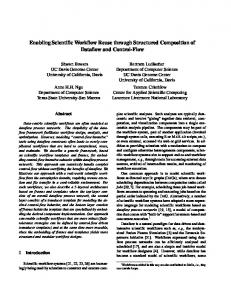
Fig. 1. The Greater Yellowstone Ecosystem study area by land management type. The black outline shows the National Park Service boundary for reference [2-column graphic, color-reproduction online only].

42

N.B. Piekielek et al. / Ecological Informatics 30 (2015) 40–48

sandy with poor water-holding capacity and little nutrient availability to support plant growth (Despain, 1990). Soils throughout the surrounding mountains are often of andesitic volcanic origin and tend to be dominated by clays, have higher water-holding capacities and are comparatively nutrient rich. The climate of the GYE has already begun to change relative to periods prior to 1980, with spring and summer temperatures approximately b1 °C warmer and reduced spring and summer snowpack (Westerling et al., 2011). The future climate of the GYE is expected to be warmer and drier than present (Chang et al., 2014). More complete descriptions of the climate, major vegetation types, and soils and topography of the GYE are provided by Brown et al. (2006) and Despain (1990). 2.2. Focal species The present study focused on the dominant vegetation species of four elevation zones being sagebrush communities (up to ~1900 m), lower treeline forests (up to ~ 2200 m), montane forests (up to ~ 2500 m), and upper treeline forests (up to ~3000 m). Sagebrush tends to occupy areas just downslope of treeline as a result of its ability to persist on well-drained soils that have a soil water deficit late in the growing season (Despain, 1990; Schlaepfer et al., 2012). Multiple species of sagebrush were all grouped into a single sagebrush community category for the present study. These species included: big sagebrush (Artemesia tridentata Nutt.), mountain big sagebrush (A. tridentata Nutt. spp. vaseyana), threetip sagebrush (A. tridentata Rydb. ssp. tripartita), Wyoming big sagebrush (A. tridentata Nutt. spp. wyomingensis), and basin big sagebrush (A. tridentata Nutt. spp. tridentata) (http://plants.usda. gov/). Lower treeline species included limber pine (Pinus flexilis) that is often found on steep, dry, rocky soils in toe slope settings (Means, 2011), and three species of juniper (Juniperus scopulorum, Juniperus occidentalis, and Juniperus osteosperma) that are generally well-adapted to hot and dry growing conditions (Despain, 1990). All juniper species were grouped into a single juniper community category for the present study. Montane forest species included lodgepole pine (Pinus contorta), Douglas fir (P. menziesii), and quaking aspen (Populus tremuloides). Montane forests included a mix of species that require deep nutrient rich soils, longer growing seasons, and adequate moisture (Douglas fir and aspen), and those that are comparatively cold and drought hardy and can tolerate lower soil nutrients (lodgepole pine). Soil properties are thought to determine the membership of montane forests across the Yellowstone plateau with lodgepole pine present on the nutrient poor sandy soils of rhyolitic parent material to the exclusion of Douglas fir and at higher elevations Englemann spruce and subalpine fir (Brown et al., 2006; Coops and Waring, 2010; Littell et al., 2008; McLane et al., 2011). The highest elevation forests occur below an upper treeline that is the result of cold temperature limitations and long durations of annual snow cover as well as shallow soils and/or an absence of soil substrate where there are rock outcroppings (Schrag et al., 2008). Typical upper treeline forest species include subalpine fir (Abies lasciocarpa), Englemann spruce (Picea engelmannii), and whitebark pine (Pinus albicaulis). Whitebark pine was not included in the present study because it was considered in a companion study (Chang et al., 2014).

The precise locations of FIA plots are protected. Imprecise plot location can affect the quality of SDMs by associating species with habitat conditions that do not actually support them (Gibson et al., 2013). A study that examined the effect of building SDMs with precise versus imprecise FIA plot location data found little effect, with a few exceptions (Gibson et al., 2013). One exception was for a species considered in the present study (J. occidentalis). As such, we undertook two additional data preparation steps. First, we compared the field measured plot elevation reported in the FIA database to the elevation of the plot's imprecise location by intersecting it with a 30-m digital elevation model and eliminated plots that exhibited more than a 333-m discrepancy. This was similar to what has been done by other studies in the region (Coops and Waring, 2010). Second, we screened our presence and absence data with a modeled data product produced with precise FIA plot locations (Wilson et al., 2012). Finally, to maintain sample independence, which would have been violated by associating multiple presence/absence observations with the exact same environmental conditions (i.e., within the same predictor grid cell), we retained only one FIA plot for each predictor grid cell. Where there was a presence and absence observation within a single predictor cell the presence observation was retained in order to identify the broadest possible environmental tolerances for each species. We used observations from 2489 FIA plots to build forest SDMs and 1374 plots to build sagebrush SDMs. We chose to limit the area of analysis to the GYE rather than entire species ranges because more detailed predictor data were available across this study domain, some species exhibit distinct genotypes that are adapted to local conditions and we wanted to produce results for a management relevant study area (i.e., the area cross which management action could conceivably have an impact). The choice of a limited study area may have identified species tolerances that were narrower than had we examined their entire range. Narrower than actual tolerances would lead to inflated potential impact (i.e., change in distribution area) when projected to future conditions. Given these limitations and recognizing the short-comings of a correlative study, we focus our discussion on potential impacts of species and communities relative to one and other rather than on the specific magnitude of projected range expansion and contraction.

Table 1 Environmental predictors used to model probability of occurrence for eight species in the Greater Yellowstone Ecosystem under current and projected future climate change scenarios. Predictor

Abbreviation

Data source

August soil moisture deficit

deft9

April snowpack

pack4

June soil moisture

soilm6

Fraction of sand in top 100 cm of soil Fraction of rock by volume in the top 100 cm of soil Direct incoming solar radiation

sandfract

PRISM/CMIP5 temperature, precipitation, soils and topography as input to water-balance model (Lutz et al., 2010) PRISM/CMIP5 temperature, precipitation, soils and topography as input to water-balance model (Lutz et al., 2010) PRISM/CMIP5 temperature, precipitation, soils and topography as input to water-balance model (Lutz et al., 2010) CONUS-SOIL (Miller and White, 1998)

rckvol

CONUS-SOIL (Miller and White, 1998)

srad

USGS 30-meter digital elevation model as input to ArcGIS Spatial Analysis tools (ESRI, 2009) USGS 30-meter digital elevation model as input to ArcGIS Spatial Analysis tools (ESRI, 2009)

2.3. Response data We derived presence and absence data for each species from the U.S. Forest Service Forest Inventory and Analysis (FIA) program database (http://apps.fs.fed.us/fiadb-downloads/datamart.html). The FIA program employs a regular gridded sampling design with one field plot for approximately every 2500 ha. Individual tree species and measurements are recorded during field visits for trees that are larger than 12.7 cm diameter at breast height. Information on understory species like sagebrush is recorded for a subset of FIA plots (see O'Connell, et al., 2012 for a description of FIA sampling methods).

Topographic wetness index

twi

N.B. Piekielek et al. / Ecological Informatics 30 (2015) 40–48

2.4. Predictor data To expand on prior SDM efforts and test a suite of predictors that should better represent the direct effects of climate on vegetation we derived predictor data related to monthly water-balance, soils and topography at a 30 arc sec spatial resolution (Table 1). Estimates of monthly temperature and precipitation that were inputs to a waterbalance model (sensu Lutz et al., 2010) came from the gridded Parameter-elevation Regressions on Independent Slopes Model dataset (PRISM Climate Group, Oregon State University, http://prism. oregonstate.edu). PRISM data represent interpolations of weather station observations based on location, elevation and other predictors of spatial variation in climate at regional scales (Daly et al., 2008). The water-balance model was a dynamic “bucket model” that added soil water or snowpack on a monthly time step and consumed available soil moisture (or released it as runoff or groundwater recharge) using approximated rates of evapotranspiration based on temperature with adjustments for latitude, slope, and aspect. A dynamic water-balance model that carried snow and soil moisture forward from one month to the next was thought to be an important improvement over temperature and precipitation predictors in the GYE because snow dynamics play a large role in controlling seasonal soil moisture availability. Water-balance predictors were also found to be important in a companion study (Chang et al., 2014). Water-balance predictors were summarized as 30-year monthly averages for the time-period 1951–1980. To represent spatial variation in soil properties we used CONUS-SOIL data from Miller and White (1998). These data describe soil physical and chemical properties that likely limit the distributions of some species and influence the outcomes of local biotic interactions such as competition (Despain, 1990). Soil predictors included the fraction by volume of rock fragments (larger than 2 mm unattached) and sand in the top 100 cm of surface soil. From USGS 30 meter digital elevation models (Gesch et al., 2009) and ArcGIS 9.3 Spatial Analyst tools (ESRI, 2009) we derived a topographic wetness index, and direct solar radiation predictors. Soils and topography were included in the present study because they are of known local importance to forest community membership (Despain, 1990; Schrag et al., 2008), however, these variables have not been included in prior national and continental scale studies. 2.5. Future climate data To project future species distributions we chose nine GCMs based on their ability to match 20th century weather observations in the region (Rupp et al., 2013) (Table 2). For each GCM, we also used a high (8.5) and low (4.5) representative concentration pathway (RCP) that refers to the amount of anthropogenic climate forcing in watts per square meter. The RCP 8.5 scenario is consistent with increases in atmospheric greenhouse gases at rates similar to present, whereas the RCP 4.5 Table 2 List of nine global climate models chosen based on their mean error relative to observed 20th century climate in the region as evaluated by Rupp et al. (2013). Model name CESM1-CAM5 CESM1-BGC CCSM4 CNRM-CM5

Developer

Community Earth System Model Contributors Community Earth System Model Contributors Community Earth System Model Contributors Centre National de Recherches Météorologiques/Centre Européen de Recherche et Formation Avancée en Calcul Scientifique HadGEM2-AO National Institute of Meteorological Research/Korea Meteorological Administration HadGEM2-ES Met Office Hadley Centre (additional HadGEM2-ES realizations contributed by Instituto Nacional de Pesquisas Espaciais) HadGEM2-CC Met Office Hadley Centre (additional HadGEM2-ES realizations contributed by Instituto Nacional de Pesquisas Espaciais) CMCC-CM Centro Euro-Mediterraneo per I Cambiamenti Climatici CanESM2 Canadian Centre for Climate Modelling and Analysis

43

scenario would require aggressive and coordinated reductions in global greenhouse gas emissions (Moss et al., 2010). Monthly projected future temperature and precipitation data were downloaded from the NASA NCCS THREDDS website (https://cds.nccs.nasa.gov/nex/) where downscaling was performed according to Thrasher et al. (2013). Future habitat was considered to be where SDMs run with at least five of nine (i.e., a simple majority) GCM inputs agreed on species presence. We also considered other threshold levels of agreement varying from one GCM to all nine GCMs and reported the variation in future suitable habitat area.

2.6. Modeling methods We used a freely available open source scientific workflow software VisTrails (Freire and Silva, 2012), that has been customized for use in SDM studies using a set of add-on tools that comprise the Software for Assisted Habitat Modeling (SAHM) (Morisette et al., 2013; https:// www.fort.usgs.gov/products/23403). VISTRAILS:SAHM provides users with tools for data preprocessing including automated reprojection, aggregation, resampling and subsetting of predictor data to match a template layer. VISTRAILS:SAHM users can select one of five different statistical SDM methods. Upon running a model, the VISTRAILS:SAHM tool produces model diagnostics including the generation of response curves that graphically represent the relationships between predictors and response that are represented in models. To save a record of the data used and workflow provenance, VISTRAILS:SAHM saves the input parameters and outputs of each model run so that a user can easily recreate any exploratory step and transfer final models to other interested researchers or natural resource managers. The goal of model construction was to identify a common set of predictors that performed well for all species in terms of common SDM diagnostics and matching our understanding of GYE ecology. Model construction was performed as follows. We first conducted a literature review of the environmental factors that have been hypothesized to limit each species. We next searched for the best available data to represent these predictors. Many predictors were found to be collinear. Collinearity can increase model coefficient standard errors and lead to large model prediction errors. We therefore, selected only predictors that were less strongly correlated (considered b 0.7 of the maximum Pearson, Spearman, and Kendall's correlation coefficients). After extensive exploratory analyses of different statistical methods and predictor sets, we chose to use multivariate adaptive regression splines (MARS) (Leathwick et al., 2006) to build SDMs. MARS methods fit non-linear relationships between environmental predictors and species presence with piecewise basis functions across multiple breakpoints (i.e., knot points) in an intentionally overfit forward stepwise manner and then prunes these based on their contribution to the model. Final binary occurrence maps were produced using a probability of presence threshold so that sensitivity (i.e., true positive rate) and specificity (i.e., true negative rate) were approximately equal. To evaluate competing models, we produced three typical SDM diagnostics through a 33%, 10-fold cross-validation. In cross-validation, models were trained on an approximately random selection of 67% of the dataset and model performance evaluated against the withheld 33% (Leathwick et al., 2006). This was repeated ten times and model diagnostics were reported as the average of all ten steps. We also examined response curves, which graphically represent the relationship between model predictors and fitted values (i.e., probabilities of presence). Response curves that are truncated, or suffer from anomalies at sampled range edges (e.g., a sudden change in the relationship from negative to positive), can lead to results that are inconsistent with ecological understanding (Anderson, 2013). Models that produced response curves that were inconsistent with ecological understanding or that produced anomalies were thrown out, even if they exhibited good model fit based on other model diagnostics.

44

N.B. Piekielek et al. / Ecological Informatics 30 (2015) 40–48

For diagnostics, we produced the area under the receiver operating characteristic curve (AUC) that ranges from 0.5 to 1.0. An AUC of 0.5 indicates performance no better than random and 1.0 indicates perfect model prediction. AUC measures above approximately 0.7 are generally considered to be good and above 0.9 are excellent (Franklin, 2009, although see Lobo et al., 2008 for a critique of AUC). AUC scores quantify the discriminatory power of models however, additional important aspects of SDM performance include accuracy (of probabilities of presence), and generalizability. As such, we also examined SDM calibration, and predictor importance. Calibration plots graph the model predicted probability of presence versus the observed prevalence from cross-validation of testing points (see Vaughan and Ormerod, 2005 for a more complete description of calibration plots). We reported the slope and intercept of calibration plots where an intercept of ‘0’ and slope of ‘1’ indicate perfect model accuracy. Variable importance scores were quantified as one minus the correlation between the original predictions and predictions produced with a single variable permuted so that low correlations indicate that the permuted variable was important. In addition to aiding model interpretation, lower predictor variable importance in testing versus training data can indicate that a particular predictor–response relationship does not generalize well to other conditions. The final step in model construction applied final models to contemporary environmental conditions to produce a spatially continuous distribution map for each species. 2.7. Projecting future probability of occurrence We used SDMs to project future probabilities of occurrence for each species under eighteen climate change scenarios (nine GCMs and two RCPs). Future projections were performed for three 30-year periods referred to by their ending year (e.g., 2040, 2070, and 2099). The resulting current and future species distributions were referred to in three ways: 1) core habitat, areas that were always projected to be within the species range; 2) deteriorating habitat, areas that were projected to change from being within the species range to outside of its range in any of the three future time periods; and 3) expanding habitat, areas that were projected to be outside of a species range under current conditions and to be within a species range in future conditions. To highlight

areas of agreement among GCMs and delineate where active management is most feasible based on current management jurisdiction and policy, we used a GIS to produce summary statistics (area, mean elevation of species distribution, and management jurisdiction) where the majority (at least five out of nine possible) GCMs predicted species occurrence. This was done for each RCP separately. To examine the effect of focusing only on locations where the majority of GCM results agree, we also reported the standard deviation of summary statistics based on different levels of GCM agreement (varied one through nine possible) divided by the total predicted currently suitable area. 3. Results 3.1. Model results The discriminatory power of final models as measured by AUC was good (N0.7) or excellent (N0.9) for all species except for limber pine (0.655) (Table 3). The accuracy of models as measured by the slope and intercept of calibration plots was good (slopes within 0.1 of 1, intercepts within 0.1 of 0) for all models except for sagebrush (slope = 0.855, intercept = − 0.214) and limber pine (slope = 0.755, intercept = −0.487). Response curves were increasing, decreasing or unimodal (Table 4). Average August soil moisture deficit (deft9), April snowpack (pack4) and the fraction of sand in surface soils (sandfract) were among the most important predictor variables across all species SDMs. 3.2. Projected responses to climate change When models were used to project future distributions under climate change scenarios lower elevation species expanded their total area while montane and upper treeline species were projected to have deteriorating habitat area. For every species in the study, expanding habitat was projected to be on average in higher elevation settings than contemporary habitat which led to projected increases in area on federal restricted lands and decreases in area on federal general lands (Table 5).

Table 3 Diagnostics of forest and shrub species distribution models in the Greater Yellowstone Ecosystem. Model accuracy here is represented by the slope (α) and intercept (β) of calibration plots. Species

Code

Number of present observations (proportion prevalence) Model discrimination Model accuracy AUC

Calibration

Sagebrush community Artemesia tridentata Artemesia tridentata spp. Vaseyana Artemesia tridentata Rydb. ssp. Tripartite Artemesia tridentata spp. Wyomingensis Artemesia tridentata spp. tridentata

artr

251 (0.10)

0.731

α = −0.214 β = 0.855

198 (0.08) 266 (0.11)

0.961

α = −0.0164 β = 1.03 α = −0.487 β = 0.755

Lower treeline Juniper community jusc Juniperus scopulorum Juniperus occidentalis Juniperus osteosperma Limber pine pifl

Montane Aspen Douglas fir Lodgepole pine

potr

417 (0.17) psme 863 (0.35) pico 1190 (0.49)

Upper treeline Engelmann spruce

pien

Subalpine fir

abla

962 (0.39) 533 (0.21)

0.655

0.863 0.777 0.768

0.765 0.857

α = −0.0208 β = 0.97 α = −0.0343 β = 0.942 α = −0.00228 β = 0.962 α = −0.0164 β = 0.94 α = −0.0147 β = 0.979

N.B. Piekielek et al. / Ecological Informatics 30 (2015) 40–48 Table 4 Predictor variables used in multivariate adaptive regression spline models and the shape of their relationship to probability of presence through the generation of response curves. Superscripts show the rank order of variable importance (from high to low) in model testing against a withheld portion of the dataset. Increasing and decreasing responses represented approximately linear positive and negative relationships, and unimodal responses were increasing and then decreasing. See Table 1 for predictor abbreviations. Species

Predictors by shape of relationship Increasing

Sagebrush deft91; srad3; community rckvol4; soilm66

Decreasing

Unimodal

pack42

sandfract5

Lower treeline Juniper community Limber pine sandfract4

pack45; srad6

rckvol1; deft92; soilm63

Montane Aspen

rckvol2

deft91; pack43; sandfract4; soilm65 pack41; deft93

Douglas fir

twi4

Lodgepole pine Upper treeline Engelmann pack44; srad5; twi6 spruce Subalpine fir srad3

pack41 ; twi2

srad5; soilm66; sandfract2; rckvol7 soilm62

sandfract1; deft93; pack44; srad5; rckvol6

deft91; soilm67

rckvol2; sandfract3

sandfract1; deft96

pack42; soilm64; rckvol5

Upper treeline species were projected to experience the most dramatic deterioration of habitat area (mean 85% decrease, range 80%– 90%), when calculated as present day compared to RCP 8.5 for the 2099 period (Figs. 2 and 3) (all summaries that follow are for the same comparison). Montane species also showed substantial projected deterioration in habitat area with an average decrease of 73% (range 60%–85%). Lower treeline species exhibited a mix of projected responses with limber pine projecting a 29% deterioration and juniper a projected expansion (55%). Sagebrush was projected to have a 40% expansion in habitat area although note some small areas of deterioration in contrast to juniper for which there was no projected deterioration (Fig. 2). Projected change in the mean elevation of distributions of montane species moved up an average of 413 m (but lodgepole pine only 298 m), upper treeline species an average of 375 m, lower treeline species an average of 269 m, and sagebrush 200 m. The two emissions scenarios agreed on likely future outcomes although using projections based on RCP 8.5 resulted in more rapid and dramatic reductions in projected habitat area for deteriorating habitat species and somewhat larger expansion of distribution area for expanding species. 3.3. Implications for management actions The proportion of species distributions on federal restricted lands was projected to increase for all species and climate change scenarios (Table 5). Upper treeline species distributions in particular, were projected to move up in elevation from federal general to federal restricted lands. The proportion of species distributions on general federal lands was projected to increase for lower elevation species both from distribution expansion (e.g., sagebrush, juniper) and projected changes in mean elevation (e.g., limber pine, aspen and Douglas fir). By the 2099 time period under RCP 8.5, more than half of the projected sagebrush and juniper distributions were on federal lands (combining federal general and federal restricted), compared to 42% and 33% at present. 4. Discussion Projected decreases in spring and summer snowpack along with increasing late season soil moisture deficit over the course of the next century (Chang et al., 2014) should result in a longer and drier growing

45

season than present and general deterioration of forest habitat in the GYE. This is consistent with the results of other studies that associated expected climate changes with projected increases in wildlife activity (Westerling et al., 2011) and forest pest outbreaks (Macfarlane et al., 2012). Some tree species may be able to track their preferred climate to higher elevations (assuming no dispersal or other limitations), although this does not guarantee that soil conditions at higher elevations will be amenable to forest establishment. As projected distributions of focal species migrated up in elevation they became better represented on federal restricted lands where management options are currently limited by agency policy. Uncertainties in modeling results along with continually changing research objectives and natural resource management staffs make it imperative that the relationships between predictors and response used to build ecological models are easily understood and that models are easily constructed and modified (i.e., reproducible) in an adaptive management framework. Scientific workflow software like VisTrails:SAHM show great potential to alleviate some of the technical challenges of modeling climate change impacts to support natural resource management decision-making. The results of the present study refined our understanding of the environmental drivers of vegetation distributions in the GYE by identifying the seasonal climate and soil conditions that structure communities across four elevation zones. Results suggested that upper treeline is the result of lengthy periods of snow cover that limit forest species establishment and lower treeline is a response to seasonal water deficit. Juniper presents an exception to this pattern in that its ability to draw from deep soil water stores combined with post European settlement fire exclusion has resulted in juniper invasion of sagebrush communities (i.e., below treeline) throughout much of the Western Cordillera, including the GYE (Leffler and Caldwell, 2005; Lyford et al., 2003). Contrary to prior studies that show future climate of the Yellowstone plateau being most suitable for present day Great Basin shrub/scrub communities (e.g., Rehfeldt et al., 2012), the present results suggested that future climate may benefit juniper communities, potentially at the expense of sagebrush (Davies et al., 2014). This difference was the result of a focus on species and genotypes that are currently present in the GYE (Great Basin shrub/scrub was not considered). A principal uncertainty in modeling montane forest habitat concerned interactions between soil properties and climate. Under current climate conditions, Douglas fir, subalpine fir, and Engelmann spruce at the lower end of their range are presently excluded from portions of the Yellowstone plateau by rhyolitic (i.e., sandy with poor nutrient content) soils. It is not clear whether this is through a competitive interaction with lodgepole pine, a complex interaction with climate, or whether they simply cannot grow on rhyolitic soils. Under the RCP 4.5 scenario of only moderate climate change, the Douglas fir distribution was projected to move upslope to occupy a core area across much of the Yellowstone plateau whereas under the RCP 8.5 scenario the projected Douglas fir distribution covered only a small portion of the Yellowstone plateau. This result was similar to that of Schrag et al. (2008) who also considered soil conditions and described opposing conclusions on the fate of upper treeline species depending on whether future precipitation increased or decreased. Under a future warmer and wetter climate, it may be that the rhyolitic soils of the Yellowstone plateau become suitable for Douglas fir, although this seems unlikely based on current observations. The calibration of more local scale models and/ or field experimentation (e.g., common garden experiments) would shed light on the likely future fate of Douglas fir on the Yellowstone plateau. Upper treeline species are almost certainly vulnerable to climate change and the incorporation of an estimate of future snowpack increased our confidence in this result. Upper treeline species may be squeezed between competitively dominant species moving upslope (like Douglas fir if it can occupy the Yellowstone plateau) and either the tops of mountains and/or unfavorable upslope conditions (Bell et al., 2014). Although the present study included rock volume as a

46

N.B. Piekielek et al. / Ecological Informatics 30 (2015) 40–48

Table 5 Area and location of projected suitable habitat by species and RCP scenario based on majority agreement of nine GCMs. Area is presented in square kilometers for current and as percentage change from current for projected future. Management zones are: 1 = private; 2 = private protected and nonfederal public; 3 = federal general; 4 = federal restricted; 5 = other. Elevation is in meters. In parentheses following change in area percentages are standard deviations in area change when agreement among GCMs is varied from 1 (at least one GCM projects species occurrence), to nine (all GCMs considered have to project species occurrence). Species

Present

2040

2070

2099

Area (percent by management Area (percent by management zones) Area (percent by management zones) Area (percent by management zones) zones 1, 2, 3, 4, 5) RCP 4.5 Sagebrush community 132,252 (50, 2, 38, 4, 6) Elevation (range) 1795 (897–3230) Lower treeline Juniper community Limber pine

Montane Aspen Douglas fir Lodgepole pine

Upper treeline Engelmann spruce Subalpine fir

+17% (+/−10) (43, 2, 41, 8, 6) 1879 (897–3608)

+23% (+/−15) (42, 2, 41, 9, 6) 1905 (897–3608)

+31% (+/−16) (40, 2, 41, 12, 5) 1940 (897–3608)

133,727 (58, 2, 31, 2, 7) 1684 (893–2849) 104,874 (41, 2, 34, 17, 6) 2013 (917–4015)

+18% (+/−10) (53, 2, 35, 4, 6) 1757 (893–3195) −13% (+/−12) (33, 3, 38, 22, 4) 2136 (917–4015)

+26% (+/−15) (50, 2, 37, 5, 6) 1790 (893–3195) −8% (+/−19) (29, 2, 42, 22, 5) 2184 (917–4015)

+32% (+/−15) (48, 2, 38, 6, 6) 1815 (893–3246) −22% (+/−20) (25, 2, 44, 24, 5) 2231 (1007–4015)

61,028 (38, 1, 50, 9, 2) 2091 (1048–3117) 78,229 (34, 2, 47, 14, 3) 2086 (992–3833) 54,199 (3, 0, 46, 49, 2) 2460 (1736–3833)

−1% (+/−25) (24, 0, 52, 23, 1) 2241 (1059–3512) −35% (+/−16) (15, 2, 55, 27, 1) 2283 (1099–3734) −28% (+/−24) (1, 0, 36, 62, 1) 2560 (1811–3867)

−5% (+/−32) (19, 0, 49, 30, 2) 2301 (1135–3512) −38% (+/−25) (11, 1, 55, 32, 1) 2341 (1099–3577) −42% (+/−36) (0, 0, 30, 69, 1) 2602 (1896–3842)

−10% (+/−31) (15, 0, 45, 40, 0) 2399 (1135–3772) −53% (+/−26) (6, 0, 52, 41, 1) 2429 (1110–3577) −50% (+/−38) (0, 0, 24, 75, 1) 2631 (1964–3867)

53,843 (1, 0, 30, 66, 3) 2712 (1123–4015) 42,144 (0, 0, 24, 72, 4) 2797 (1368–4015)

−46% (+/−24) (0, 0 , 22, 75, 3) 2864 (1123–4015) −43% (+/−30) (0, 0, 19, 75, 6) 2929 (1354–4015)

−61% (+/−36) (0, 0, 18, 79, 3) 2934 (1123–4015) −56% (+/−46) (0, 0, 18, 76, 6) 2982 (1354–4015)

−77% (+/−38) (0, 0, 16, 81, 3) 3021 (1123–4015) −68% (+/−49) (0, 0, 16, 76, 8) 3038 (1354–4015)

+18% (+/−9) (43, 2, 41, 7, 7) 1878 (897–3608)

+28% (+/−16) (40, 2, 41, 11, 6) 1929 (897–3711)

+40% (+/−17) (37, 1, 40, 16, 6) 1995 (897–3771)

133,727 (58, 2, 31, 2, 7) 1684 (893–2849) 104,874 (41, 2, 34, 17, 6) 2013 (917–4015)

+16% (+/−9) (54, 2, 34, 4, 6) 1749 (893–3195) −15% (+/−12) (32, 3, 38, 22, 5) 2147 (917–4015)

+32% (+/−16) (48, 2, 38, 6, 6) 1813 (893–3246) −37% (+/−21) (29, 3, 43, 21, 4) 2189 (971–4015)

+55% (+/−16) (41, 1, 39, 14, 5) 1928 (893–3608) −29% (+/−21) (17, 2, 49, 28, 4) 2307 (1071–4015)

61,028 (38, 1, 50, 9, 2) 2091 (1048–3117) 78,229 (34, 2, 47, 14, 3) 2086 (992–3833) 54,199 (3, 0, 46, 49, 2) 2460 (1736–3833)

+7% (+/−25) (24, 0, 52, 22, 2) 2234 (1059–3512) −37% (+/−16) (15, 2, 55, 27, 1) 2284 (1099–3577) −26% (+/−23) (1, 0, 36, 62, 0) 2550 (1811–3867)

−1% (+/−23) (15, 0, 46, 38, 1) 2382 (1135–3772) −63% (+/−27) (8, 0, 53, 37, 2) 2394 (1110–3577) −53% (+/−40) (0, 0, 24, 76, 0) 2622 (1964–3842)

−60% (+/−36) (12, 0, 27, 61, 0) 2560 (1356–3772) −73% (+/−28) (2, 0, 43, 53, 2) 2559 (1121–3714) −85% (+/−41) (0, 0, 11, 89, 0) 2758 (2130–3833)

53,843 (1, 0, 30, 66, 3) 2712 (1123–4015) 42,144 (0, 0, 24, 72, 4) 2797 (1368–4015)

−47% (+/−23) (0, 0, 22, 76, 2) 2864 (1123–4015) −44% (+/−29) (0, 0, 20, 75, 5) 2930 (1354–4015)

−77% (+/−40) (1, 0, 16, 80, 3) 3016 (1123–4015) −66% (+/−51) (0, 0, 16, 77, 7) 3036 (1354–4015)

−90% (+/−41) (1, 0, 12, 84, 3) 3145 (1123–4015) −80% (+/−52) (0, 0, 12, 80, 8) 3114 (1394–4015)

RCP 8.5 Sagebrush community 132,252 (50, 2, 38, 4, 6) Elevation (range) 1795 (897–3230) Lower treeline Juniper community Limber pine

Montane Aspen Douglas fir Lodgepole pine

Upper treeline Engelmann spruce Subalpine fir

predictor, upper treeline species models projected future distributions up to the highest elevations in the study area where a lack of soil in many places (i.e., exposed rock outcroppings) does not presently support forest establishment. Upper treeline models missed an upper elevation habitat threshold due to a paucity of forest inventory observations above treeline and therefore a more weak response to high rock volume than we understand. There is evidence that upper treeline species can rapidly invade alpine habitats where there are suitable soil conditions and when climate is conducive, such as the climate that is expected in the future of the American mountain west (Grant, 2012). Although an expansion of our study area to include the northern range limits of upper treeline species may have alleviated this issue by including upper elevation climatic limits to forest distributions, more observations of forest dynamics at and above treeline remains sorely needed to better understand upper treeline dynamics within the context of climate change impacts. Both poor model performance and disagreement among GCM projections limited our ability to draw conclusions from some SDM results. The limber pine SDM in particular did not perform well (low AUC, poor

model calibration), perhaps in part due to low species prevalence. Projections of change in distribution area varied widely for a few species when the level of agreement between GCMs was changed from low levels to high levels of agreement required to project future occurrence. This led to some area change projections whose uncertainty (standard deviation of projected area change when agreement was varied), crossed zero (e.g., the results for aspen and limber pine). There was also substantial variation in the lodgepole pine results and to a lesser extent the results for subalpine fir. However, the aspen, limber pine and lodgepole models were the only three for which projections of distribution area change actually changed sign (i.e., deteriorating to expanding or vice versa) when levels of GCM agreement were varied while other species models merely varied (sometimes greatly), in the extent to which they projected expansion or deterioration of distributions. Examinations of uncertainty such as the one employed here highlight the levels of disagreement among current GCM projections and the ways in which they can decrease our confidence in SDM results. Modeling the potential ecological impacts of climate change to support natural resource management decision-making presents a host of

N.B. Piekielek et al. / Ecological Informatics 30 (2015) 40–48

47

Fig. 2. Current and projected future (RCP 8.5, majority agreement among GCMs) suitable habitat for eight vegetation species across four elevation zones of the Greater Yellowstone Ecosystem. Species abbreviations are presented in Table 3. The black outline shows the National Park Service boundary [2-column fitting image, color reproduction online only].

technical challenges during model formulation, evaluation, and technology transfer phases of a project. Many of these challenges are alleviated by the use of custom scientific workflow software like VisTrails:SAHM that enables the relatively rapid production of ecologically defensible and well-documented SDMs. Time saved by custom software on the model formulation phase of a project can be used to more critically evaluate future projection results, such as by zones of management jurisdiction in a GIS. The data and workflow provenance automatically captured by scientific workflow software should also aid in the technology transfer of SDM results, such as to natural resource management agencies that want to run models in their own computing environment, update results with new or different GCMs, or develop and test their own ecological hypotheses in an adaptive management framework. By engaging and empowering natural resource managers to also be producers of climate change understanding after the end of a sponsored research

project, they will likely be in a better position to develop successful climate adaptation strategies. Responding to expected future climate change is a daunting challenge faced by today's natural resource management community. Fortunately, there is reason to be hopeful that employing a mix of currently successful strategies and new approaches may produce desirable outcomes for the GYE. For example, active management that is wellcoordinated across ownership jurisdictions like the whitebark pine strategy (GYCC, 2011) employed by the Greater Yellowstone Coordinating Committee is already making contributions to the maintenance of an important upper treeline species within the study area (GYCC, 2011). New guidance on how to conduct climate vulnerability assessments (Glick et al., 2011) and how to respond to the results of those assessments (i.e., the Climate-smart framework for conservation planning) (Stein et al., 2014) provide excellent guidance on how natural

48

N.B. Piekielek et al. / Ecological Informatics 30 (2015) 40–48

resource managers can begin to respond to expected future climate change. Acknowledgments We would like to thank the USGS North Central Climate Science Center and Jeff Morisette for funding and the creation of VisTrails:SAHM. Funding was also provided by the NASA Applied Sciences Program (10-BIOCLIM10-0034) and the Montana NSF EPSCoR Initiative. We would also like to thank Colin and Marian Talbert for their work on SAHM and their invaluable assistance in its use. We thank Linda Phillips for assistance creating graphics and D. Schlaepfer, P. Jantz and two anonymous reviewers for insightful commentson a draft of this manuscript. We acknowledge the World Climate Research Programme's Working Group on Coupled Modelling, which is responsible for CMIP, and we thank the climate modeling groups (listed in Appendix S1, Table 3 of this paper) for producing and making available their model output. For CMIP the U.S. Department of Energy's Program for Climate Model Diagnosis and Intercomparison provides coordinating support and led development of software infrastructure in partnership with the Global Organization for Earth System Science Portals. References Anderson, R.P., 2013. A framework for using niche models to estimate impacts of climate change on species distributions. Ann. N. Y. Acad. Sci. 1297, 8–28. http://dx.doi.org/10. 1111/nyas.12264. Araújo, M.B., Guisan, A., 2006. Five (or so) challenges for species distribution modelling. J. Biogeogr. 33, 1677–1688. http://dx.doi.org/10.1111/j.1365-2699.2006.01584.x. Bell, D.M., Bradford, J.B., Lauenroth, W.K., 2014. Mountain landscapes offer few opportunities for high‐elevation tree species migration. Glob. Chang. Biol. 20, 1441–1451. http://dx.doi.org/10.1111/gcb.12504. Brown, K., Hansen, A.J., Keane, R.E., Graumlich, L.J., 2006. Complex interactions shaping aspen dynamics in the Greater Yellowstone Ecosystem. Landsc. Ecol. 21, 933–951. http://dx.doi.org/10.1007/s10980-005-6190-3. Chang, T., Hansen, A.J., Piekielek, N., 2014. Patterns and variability of projected bioclimatic habitat for Pinus albicaulis in the Greater Yellowstone Area. PLoS ONE 9 (11), e111669. Coops, N.C., Waring, R.H., 2010. A process-based approach to estimate lodgepole pine (Pinus contorta Dougl.) distribution in the Pacific Northwest under climate change. Clim. Chang. 105, 313–328. http://dx.doi.org/10.1007/s10584-010-9861-2. Daly, C., Halbleib, M., Smith, J.I., Gibson, W.P., Doggett, M.K., Taylor, G.H., Pasteris, P.P., 2008. Physiographically sensitive mapping of climatological temperature and precipitation across the conterminous united states. Int. J. Climatol. 28 (15), 2031–2064. http://dx.doi.org/10.1002/joc.1688. Davies, K.W., Bates, J.D., Madsen, M.D., Nafus, A.M., 2014. Restoration of mountain big sagebrush steppe following prescribed burning to control western juniper. Environ. Manage. 53, 1015–1022. http://dx.doi.org/10.1007/s00267-014-0255-5. Despain, Don G., 1990. Yellowstone Vegetation: Consequences of Environment and History in a Natural Setting. Roberts Rinehart Publishers, Inc. ESRI, 2009. ArcGIS Desktop: Release 9.3. Environmental Systems Research Institute, Redlands, CA. Freire, J., Silva, C.T., 2012. Making computations and publications reproducible with VisTrails. Comput. Sci. Eng. http://dx.doi.org/10.1109/MCSE.2012.76 (July/August). Franklin, J., 2009. Mapping Species Distributions: Spatial Inference and Prediction. Cambridge University Press, Cambridge, UK. Gesch, D., Evans, G., Mauck, J., Hutchinson, J., Carswell Jr., W.J., 2009. The national map—elevation. U.S. Geological Survey Fact Sheet 2009–3053 (4 pp.). Gibson, J., Moisen, G., Frescino, T., Edwards, T.C., 2013. Using publicly available forest inventory data in climate-based models of tree species distribution: examining effects of true versus altered location coordinates. Ecosystems 17, 43–53. http://dx.doi.org/ 10.1007/s10021-013-9703-y. Glick, P., Stein, B.A., Edelson, N.A. (Eds.), 2011. Scanning the Conservation Horizon: A Guide to Climate Change Vulnerability Assessment. National Wildlife Federation, Washington, D.C. Grant, E., 2012. Extrinsic regime shifts drive abrupt changes in regeneration dynamics at upper treeline in the Rocky Mountains, USA. Ecol. 93, 1614–1625. http://dx.doi.org/ 10.1890/11-1220.1. Greater Yellowstone Coordinating Committee (GYCC), 2011. Whitebark Pine Subcommittee. Whitebark Pine Strategy for the Greater Yellowstone Area (41 pp.). Hansen, A.J., Piekielek, N.B., Davis, C., Haas, J., Oliff, S.T., Gross, J., Monahan, B., Theobald, D., 2014. Exposure of U. S. National Parks to land use and climate change 1900–2100. Ecol. Appl. 24, 484–502. http://dx.doi.org/10.1890/13-0905.1. Harte, J., Saleska, S., Shih, T., 2006. Shifts in plant dominance control carbon-cycle responses to experimental warming and widespread drought. Environ. Res. Lett. 1, 014001. http://dx.doi.org/10.1088/1748-9326/1/1/014001.

Knutti, R., Sedláček, J., 2012. Robustness and uncertainties in the new CMIP5 climate model projections. Nat. Clim. Chang. 3, 369–373. http://dx.doi.org/10.1038/NCLIMATE1716. Leathwick, J.R., Elith, J., Hastie, T., 2006. Comparative performance of generalized additive models and multivariate adaptive regression splines for statistical modelling of species distributions. Ecol. Model. 199, 188–196. http://dx.doi.org/10.1016/j.ecolmodel.2006. 05.022. Leffler, A.J., Caldwell, M.M., 2005. Shifts in depth of water extraction and photosynthetic capacity inferred from stable isotope proxies across an ecotone of Juniperus osteosperma (Utah juniper) and Artemisia tridentata (big sagebrush). J. Ecol. 93, 783–793. http://dx.doi.org/10.1111/j.1365-2745.2005.01014.x. Littell, J.S., Peterson, D.L., Tjoelker, M., 2008. Douglas-fir growth in mountain ecosystem: water limits tree growth from stand to region. Ecol. Monogr. 78, 349–368. http:// dx.doi.org/10.1890/07-0712.1. Lobo, J.M., Jiménez-Valverde, A., Real, R., 2008. AUC: a misleading measure of the performance of predictive distribution models. Glob. Ecol. Biogeogr. 17, 145–151. http://dx. doi.org/10.1111/j.1466-8238.2007.00358.x. Lutz, J.A., van Wagtendonk, J.W., Franklin, J.F., 2010. Climatic water deficit, tree species ranges, and climate change in Yosemite National Park. J. Biogeogr. 37, 936–950. http://dx.doi.org/10.1111/j.1365-2699.2009.02268.x. Lyford, M.E., Jackson, S.T., Betancourt, J.L., Gray, S.T., 2003. Influence of landscape structure and climate variability on a late Holocene plant migration. Ecol. Monogr. 73, 567–583. http://dx.doi.org/10.1890/03-4011. Macfarlane, W.W., Logan, J.A., Kern, W., 2012. An innovative aerial assessment of Greater Yellowstone Ecosystem mountain pine beetle-caused whitebark pine mortality. Ecol. Appl. 23 (2), 421–437. McLane, S.C., Daniels, L.D., Aitken, S.N., 2011. Climate impacts on lodgepole pine (Pinus contorta) radial growth in a provenance experiment. For. Ecol. Manag. 262, 115–123. http://dx.doi.org/10.1016/j.foreco.2011.03.007. Means, R.E., 2011. Synthesis of lower treeline limber pine (Pinus flexis) woodland knowledge, research needs, and management considerations. The future of high-elevation, five-needle white pines in Western North America. In: Keane, R.E., Tomback, D.F., Murray, M.P., Smith, C.M. (Eds.), Proceedings of the High Five Symposium, p. 376 (Missoula, MT). Miller, D.A., White, R.A., 1998. A conterminous United States multi-layer soil characteristics data set for regional climate and hydrology modeling. Earth Interact. 2. Morisette, J.T., Jarnevich, C.S., Holcombe, T.R., Talbert, C.B., Ignizio, D., Talbert, M.K., Silva, C., Koop, D., Swanson, A., Young, N.E., 2013. VisTrails:SAHM: visualization and workflow management for species habitat modeling. Ecography 36, 129–135. http://dx.doi.org/ 10.1111/j.1600-0587.2012.07815.x. Moss, R.H., Edmonds, J.A., Hibbard, K.A., Manning, M.R., Rose, S.K., Van Vuuren, D.P., et al., 2010. The next generation of scenarios for climate change research and assessment. Nature 463, 747–756. http://dx.doi.org/10.1038/nature08823. O'Connell, B.M., LaPoint, E.B., Turner, J.A., Ridley, T., Boyer, D., Wilson, A.M., Waddell, K.L., Christensen, G., Conkling, B.L., 2012. The Forest Inventory and Analysis Database: Database Description and Users Manual Version 5.1.2 for Phase 2. U.S. Department of Agriculture. Piekielek, N.B., Hansen, A.J., 2012. Extent of fragmentation of coarse-scale habitats in and around U.S. National Parks. Biol. Conserv. 155, 13–22. Rehfeldt, G.E., Crookston, N.L., Saenz-Romero, C., Cambell, E.M., 2012. North American vegetation model for land-use planning in a changing climate: a solution to large classification problems. Ecol. Appl. 22, 119–141. http://dx.doi.org/10.1890/11-0495.1. Rupp, D.E., Abatzoglou, J.T., Hegewisch, K.C., Mote, P.W., 2013. Evaluation of CMIP5 20th century climate simulations for the Pacific Northwest USA. J. Geophys. Res. Atmos. 118, 10,884–10,906. http://dx.doi.org/10.1002/jgrd.50843. Schlaepfer, D.R., Lauenroth, W.K., Bradford, J.B., 2012. Consequences of declining snow accumulation for water balance of mid-latitude dry regions. Glob. Chang. Biol. 18, 1988–1997. http://dx.doi.org/10.1111/j.1365-2486.2012.02642.x. Schrag, A.M., Bunn, A.G., Graumlich, L.J., 2008. Influence of bioclimatic variables on treeline conifer distribution in the Greater Yellowstone Ecosystem: implications for species of conservation concern. J. Biogeogr. 35, 698–710. http://dx.doi.org/10.1111/j. 1365-2699.2007.01815.x. Stein, B.A., Glick, P., Edelson, N., Staudt, A. (Eds.), 2014. Climate-smart Conservation: Putting Adaptation Principles Into Practice. National Wildlife Federation, Washington D.C. Stephenson, N.L., 1998. Actual evapotranspiration and deficit: biologically meaningful correlates of vegetation distributions across spatial scales. J. Biogeogr. 25, 855–870. http://dx.doi.org/10.1046/j.1365-2699.1998.00233.x. Thrasher, B., Xiong, J., Wang, W., Melton, F., Michaelis, A., Nemani, R., 2013. Downscaled climate projections suitable for resource management. EOS Trans. Am. Geophys. Union 94, 321–323. http://dx.doi.org/10.1002/2013EO370002. Vaughan, I.P., Ormerod, S.J., 2005. The continuing challenges of testing species distribution models. J. Appl. Ecol. 42, 720–730. http://dx.doi.org/10.1111/j.1365-2664.2005. 01052.x. Westerling, A.L., Turner, M.G., Smithwick, E.A., Romme, W.H., Ryan, M.G., 2011. Continued warming could transform Greater Yellowstone fire regimes by mid-21st century. Proc. Natl. Acad. Sci. U. S. A. 108, 13165–13170. Wilson, B.T., Lister, A.J., Riemann, R.I., 2012. A nearest-neighbor imputation approach to mapping tree species over large areas using forest inventory plots and moderate resolution raster data. For. Ecol. Manag. 271, 182–198.