Using Differential Evolution for Fine Tuning Naïve Bayesian Classifiers

Using Differential Evolution for Fine Tuning Naïve Bayesian Classifiers and its Application for Text Classification Diab M Diab, Khalil M El Hindi Department of Computer Science College of Computer and Information Sciences King Saud University P.O. Box-51178, Riyadh-11543 Kingdom of Saudi Arabia E-mail: [email protected], [email protected]

ABSTRACT The Naive Bayes (NB) learning algorithm is simple and effective in many domains including text classification. However, its performance depends on the accuracy of the estimated conditional probability terms. Sometimes these terms are hard to be accurately estimated especially when the training data is scarce. This work transforms the probability estimation problem into an optimization problem, and exploits three metaheuristic approaches to solve it. These approaches are Genetic Algorithms (GA), Simulated Annealing (SA), and Differential Evolution (DE). We also propose a novel DE algorithm that uses multiparent mutation and crossover operations (MPDE) and three different methods to select the final solution. We create an initial population by manipulating the solution generated by a method used for fine-tuning the NB. We evaluate the proposed methods by using their resulted solutions to build NB classifiers and compare their results with the results obtained from classical NB and Fine-Tuning Naïve Bayesian (FTNB) algorithm using 53 UCI benchmark data sets. We name these obtained classifiers NBGA, NBSA, NBDE, and NB-MPDE respectively. We also evaluate the performance NB-MPDE for text-classification using 18 text-classification data sets, and compare its results with the results obtained from FTNB, BNB, and MNB. The experimental results show that using DE in general and the proposed MPDE algorithm in particular are more convenient for fine-tuning NB than all other methods, including the other two metaheuristic methods (GA, and SA). They also indicate that NB-MPDE achieves superiority over classical NB, FTNB, NBDE, NBGA, NBSA, MNB, and BNB.

Keywords: Fine Tuning Naïve Bayes, Differential Evolution, Text Classification, Improving estimated probabilities, Multi-parent mutation, Multi-parent crossover, Genetic algorithm, Simulated Annealing, Bernoulli NB, Multinomial NB. 1

1. INTRODUCTION: In spite of the existence of many classifiers [1–20], probabilistic classifiers (like NB classifiers) are still among the most widely used classifiers for their simplicity, and robustness [21–23]. The Naïve Bayesian learning algorithm is one of the most popular, simple, and practical machine learning algorithms. It is considered among the top 10 performing data mining algorithms[24]. It performs surprisingly well compared to other more sophisticated classification methods in many domains [25–32], especially in text classification. The NB algorithm is based on the Bayesian theorem with a conditional independence assumption between predictors. Simply it uses training data set to estimate the probability terms that are needed for classification. The performance of the NB algorithm depends on the accurate estimation of the required probability terms, which could be a major challenge especially when the training data is scarce as usual. This issue has been addressed in the literature using different methods such as instance cloning [33–35],and fine-tuning the NB (FTNB) [36,37]. This work transforms the probability estimation problem into an optimization problem, and exploits three metaheuristic approaches to solve it. These approaches are Genetic Algorithms (GA), Simulated Annealing (SA), and Differential Evolution (DE). We also propose a novel DE algorithm that uses a multi-parent mutation and crossover operations (MPDE), evaluate and compare these methods by using their resulted solutions to build NB classifiers. We name these new NB classifiers NBGA, NBSA, NBDE, and NB-MPDE respectively. The rest of the paper is structured as follows: Section 2 is the theoretical foundation section in which we discuss the classical Naïve Bayes (NB) with two other versions of NB algorithms dedicated for text classification domain. We also discuss Differential Evolution (DE), Simulated Annealing (SA), and Genetic Algorithm (GA). in Section 3, we discuss related work. In section 4, we show how to use DE and MPDE to fine tune the NB algorithm. Section 5 presents and analyzes the results. Section 6 is the conclusion section.

2. THEORETICAL FOUNDATIONS In this section, we review the theoretical material relevant for this work., we explain the classical Naïve Bayes (NB) with two other versions of NB algorithms dedicated for text classification domain. We also discuss Differential Evolution (DE), Simulated Annealing (SA), and Genetic Algorithm (GA).

2

2.1 Naïve Bayesian Learning Every instance in training set is represented as a vector of attribute values , where i = 1, … , n and 𝑎i is the value of the 𝑖𝑡ℎ attribute. Given a new unobserved instance of the form < 𝑎1 , 𝑎2 … 𝑎n >, NB assigns the class 𝑐𝑝𝑟𝑒𝑑𝑖𝑐𝑡𝑒𝑑 , which has the maximum conditional probability value computed using Bayes' rule as follows: 𝑐𝑝𝑟𝑒𝑑𝑖𝑐𝑡𝑒𝑑 = 𝑎𝑟𝑔𝑚𝑎𝑥𝑐 ∈𝐶

𝑝(𝑎1 , 𝑎2

… 𝑎n |c).𝑝(c)

𝑝(𝑎1 ,𝑎2 … 𝑎n )

……. (1)

where C is the set of all classes, 𝑝(c) is the probability of class c, 𝑝(𝑎1 , 𝑎2 … 𝑎n ) is the probability that attributes 1,2, …,n will take the values 𝑎1 , 𝑎2 … 𝑎n ,respectively, and 𝑝(𝑎1 , 𝑎2 … 𝑎n |c) is the probability that attributes 1, 2, …, n will take the values 𝑎1 , 𝑎2 … 𝑎n given that the instance is of class c. Since the denominator in formula 1 is identical for all classes, the formula can be simplified by eliminating the denominator as follows. 𝑐𝑝𝑟𝑒𝑑𝑖𝑐𝑡𝑒𝑑 = 𝑎𝑟𝑔𝑚𝑎𝑥𝑐 ∈𝐶 𝑝(𝑎1 , 𝑎2 … 𝑎n |c). 𝑝(c) ……. (2) Naïve Bayesian algorithm assumes that the instance’s attributes’ values are conditionally independent given the class value; therefore, the probability of the conjunction given the class c is just a product of the probabilities of the individual attributes’ values given c. 𝑝(𝑎1 , 𝑎2 … 𝑎n |c) = ∏ni=1 𝑝(𝑎i |c) ……. (3) Consequently, 𝑐𝑝𝑟𝑒𝑑𝑖𝑐𝑡𝑒𝑑 = 𝑎𝑟𝑔𝑚𝑎𝑥𝑐 ∈𝐶 𝑝(c). ∏ni=1 𝑝(𝑎i |c) ……. (4) where 𝑝 (c) and 𝑝(𝑎i |c) could be estimated from the training data set. If the value of one probability terms is zero, then the conditional probability of the class is also zero, no matter how large the probabilities of the other terms are. To avoid this, Laplace smoothing is usually used. 𝑝(𝑎i |c) =

𝑐𝑜𝑢𝑛𝑡(𝑎𝑖 ,𝑐)+1 𝑐𝑜𝑢𝑛𝑡(𝑐)+|𝑣|

……. (5)

where count(𝑎i , c) is the number of occurrences of the attribute i having value 𝑎i in instances of class c in the training data set, count(c) is the number of instances having class c, |v| is the number of values of attribute 𝑖.

3

2.2 Naïve Bayesian for Text-classification Text-classifications is an area in which NB performs remarkably well[17,38]. In the following two subsections we discuss two typical methods for using NB classifies for text classifications: Bernoulli Naïve Bayes and Multinomial Naïve Bayes. 2.2.1 Bernoulli Naïve Bayes Bernoulli document model is a representation of a document as a vector of binary numbers; Each binary value represents the presence or absence of certain word, taking value 1 if the corresponding word is available in the document and 0 otherwise [29,39,40]. To classify an unlabeled document D, we use the following equation: |V|

cpredicted = argmaxc ∈C p(c). ∏t=1 p(D|c) ….. (6) |V|

= argmaxc ∈C p(c). ∏𝑡=1[ bt P (wt |c) + (1 − bt )(1 − P (wt |c))] …..(7) where: P(wt |c) is the probability that the word wt occurs in a document of class c; V is the vocabulary used in all the documents, and bt is a binary value that represents the availability or absence of the corresponding word: bt =1 when word wt is available, and bt =0 when word wt is unavailable. Laplace’s law of succession is used to estimate the probability values: ̂(wt |c=k) =1+ nk (wt) ……… (8) P N +|v| k

where nk (wt ) is the number of documents of class k in which wt is available, and Nk is the total number of documents of that class. The prior probability, P(c) is a relative frequency of documents of class k. It is computed as follows: ̂(c=k) = Nk …….. (9) P N where N is the total number of documents in the training set. 2.2.2 Multinomial Naïve Bayes: Multinomial Naïve Bayesian [20,27,41] uses a vector of words to represent a document. Suppose a document, D is represented by a words vector , it is classified as follows: 𝑚

cpredicted (D) = arg maxc ∈C [log P(c) + ∑

𝑗=0

fj log P(𝑤j |c)] … … (10)

where C is the set of all possible class labels, 𝑚 is the number of words, wj (j=1, 2,…, m) is the jth word occurs in the document D, fj is the frequency count of word wj in the document D. 4

2.3 Differential Evolution Differential Evolution (DE) is a stochastic, population-based model used to optimize real parameters or real valued functions[42]. Storn and Price [43] proposed a DE algorithm as a heuristic algorithm to search for the optimal solution in large spaces of solutions. The general idea of DE is based on composing a temporary population by exploiting the individual differences of the current population. The algorithm then selects individuals which have highest fitness values from the offspring generation and the parents to form a new generation. The evolution process continues by applying three main steps: selection, recombination, and mutation. The Differential Evolution algorithm tends to move towards the optimal solution by maintaining the best individuals and eliminating the weak ones. In the mutation phase, a differential vector is computed by subtracting two or more individuals (donor vectors), and adding another individual vector (second parent) to produce a mutant vector. All individuals are randomly selected. There are many different DE schemes based on different variants of the mutation step [44]:     

DE/rand/1/bin: Xi,g+1 = X r1,g + F.( Xr2,g − Xr3,g ). DE/best/1/bin: Xi,g+1 =Xbest,g + F.( Xr1,g − Xr2,g ). DE/current to best/2/bin: Xi,g+1 = Xi,g + F.( Xbest,g − Xi,g )+ F.( Xr1,g − Xr2,g ). DE/best/2/bin: Xi,g+1 =Xbest,g + F.( Xr1,g − Xr2,g )+ F.( Xr3,g − Xr4,g ). DE/rand/2/bin: Xi,g+1 = X r1,g + F.( Xr2,g − Xr3,g )+ F.( Xr4,g − Xr5,g ).

where F is a constant number in the range )0, 2] representing the mutation rate, X i,g+1 is the mutant

vector,

Xbest,g

is

the

best

individual

of

the

current

population.

Xr1,g , Xr2,g , Xr3,g , Xr4,g , Xr5,g are randomly selected individuals from the current population, and they also should be different to each other. A trial vector is produced by applying crossover operation. In this operation, the mutant vector is mixed with the target vector based on crossover rate. Finally, the algorithm compares between the fitness value of the target vector and trial vector and passes the one with better fitness value to the next generation. The process of mutation, recombination and selection continue until a stopping criterion is reached. Figure 1 is taken from [45], it shows the details of the classical differential evaluation algorithm.

5

Algorithm DE Input : F, CR, fitness_function, termination_condition, intial_population, max_generation, final_solution_method Output : fitness_function parameter values with maximum fitness_function value 1 2 3 4 5 6 7 8 9 10 11 12 13 14

g=0 , N= size of intial_population repeat for each individual i in the population do Generate three random integers r1, r2 and r3 ∈ [1, N], with r1 ≠ r2 ≠ r3 ≠ i Generate a random integer Irand ∈ [1, n] for each dimensional variable j in one individual do Vi,j ,g+1 = Xr1,j,g + F. (Xr2,j,g − Xr3,j,g ) Vi,j,g+1 , if randj,i ≤ CR or j = Irand Ui,j ,g+1 = { Xi,j,g Otherwise end for Replace Xi,g with the child Ui,g+1 , if Ui,g+1 has better fitness_function end for g=g+1 until the termination_condition is achieved or g=max_generation if (g=max_generation) use final_solution_method for defining the parameters values

Fig 1: A classical algorithm of Differential Evolution [45]

2.4 Genetic Algorithm Genetic algorithm (GA) is a metaheuristic population-based optimization technique. In practice, genetic algorithm has a strong impact on optimization problems [26]. It uses its bio-inspired operators to find better solutions[46,47]. The algorithm starts by generating an initial population which contains M randomly selected solutions, then it uses its bio-inspired operators to generate a new population. This is performed repeatedly G times, where G is the number of generations. Figure 2 shows a GA version which creates only one offspring in each iteration [26] and it is the one we use in our empirical work.

RANDOM_SELECTION randomly selects a pair of

individuals for reproduction in accordance with a probability that is proportional to their fitness values. REPRODUCE, represents the mating between selected individuals. The crossover points along the selected individuals are randomly selected. Finally, MUTATE, is performed randomly with a small probability to introduce random modifications to the offspring. This increases the diversity of population.

6

Algorithm GA Input: initial population // a set of individuals FITNESS-FN // a function which determines the quality of the individual Output: an individual 1 repeat 2 new_population  empty set 3 for each individual i in the population do 4 x  RANDOM_SELECTION(population, FITNESS_FN) 5 y  RANDOM_SELECTION(population, FITNESS_FN) 6 child  REPRODUCE(x, y) 7 if (small random probability) then child  MUTATE(child ) 8 add child to new_population 9 population  new_population 10 end for 11 until the maximum number of generations is reached max generation number 12 return the best individual Fig 2: A classical Genetic Algorithm [26].

2.5 Simulated Annealing Algorithm Simulated annealing (SA) is a metaheuristic technique that simulates the annealing process in finding better material structures (solutions). In the early stages of annealing, the material will be heated to a very high temperature, then it is slowly cooled, and minimized the system energy. During the execution of SA, it changes its state from a random search at the beginning (i.e. at high temperature) into a greedy search (i.e. at low temperature) [26]. SA maintains a current assignment of values to the objective function variables. At each step, the temperature is cooled by some rate, COOLING, and the algorithm picks a small set of variables randomly, and assigns a random value to them. If this assignment causes improvement or does not decrease the fitness value, the algorithm accepts the assignment. Otherwise, it accepts the assignment with some probability, depending on the value of temperature, T, and how worse the new assignment is than the current assignment ΔE . If the change is not accepted, the current assignment is unchanged. This randomness in the acceptance of the new solution at high temperature (i.e. at the early stage of execution) should help the algorithm to jump out of local maxima [26]. Figure 3 shows a classical Simulated Annealing Algorithm [26]. and it is the one we use in our empirical work.

7

Algorithm SA Input: INITIAL-SOLUTION, High_Temperature COOLING// function to cool the temperature by a cooling rate Output: best solution 1 next  MAKE-NEW-SOLUTION(INITIAL-SOLUTION) 2 T  High_Temperature steps 3 current  MAKE-NEW-SOLUTION(INITIAL-SOLUTION) 4 for t  1 to High_Temperature do 5 T  COOLING[t] 6 if T 0 then current  next 10 else current  next only with probability 𝑒 ΔE /T 11 end for Fig 3: A classical Simulated Annealing Algorithm [26].

3. RELATED WORK Probabilistic classifiers like NB classifiers are among the most widely used classifiers in many domains, especially in text classification domain [21–23]. These classifiers are derived from generative probability models [23], therefore, the quality, and availability of training data set play a vital role in their performance. It should reflect the underlying distribution of the instances perfectly to support the classifier with accurate estimations for the used probability terms, and unfortunately, this situation is rarely occurred. This challenge is very critical for this family of classifiers, especially for NB classifiers. NB classifier is one of the simplest probabilistic classifiers. It is easy to implement, fast, accurate, and relatively robust. All these features enable it to be the most popular classifier in many domains [20,48,49]. The performance of NB algorithm depends on two main factors: the validity of the conditional independence assumption in the used data set, and the ability to find accurate estimations of the required probability terms. NB’s classification accuracy degrades in domains where one or both of these factors are violated. Some researchers focused on relaxing the independence assumption problem [49–53], while other researchers proposed methods to deal with the lack of training data problem and consequently, decreases the margin of errors in estimating the probability terms [54,33,35,36,55]. The first issue has been addressed in the literature by developing various Bayesian networks [51,56–58] and by using feature selection methods [54,38,59–61]. A natural extension of the 8

Naive Bayes classifier, called Tree Augmented Naive Bayes (TAN), was proposed by Friedman [57]. TAN captures the correlations between the attributes by allowing extra edges between the attributes of NB network. Qiu et al. [51] improved TAN accuracy by using conditional log likelihood (CLL) to find the augmenting arcs. Langley [59] proposed another method called Selective Naive Bayes (SBC) to improve the classification accuracy by using selected subset of attributes, on the other hand, Jiang et al. [61] use a wrapper approach for selecting attributes and carrying a random search through the whole space of attributes. Zhang et al. [38] proposed a hybrid feature selection approach that uses base classifiers to evaluate attribute subsets just like a wrapper approach, but without repeat searching for attribute subsets and building base classifiers. One more attempt to weaken the independence assumption of NB is done by Jiang et al. [49], they proposed a deep feature weighting method (DFW). In this method they incorporate the learned attribute weights into the conditional probability estimates by deeply computing attribute weighted frequencies from training data. Cloning instances [33,35] and assigning instances different weights [48,53,55,62] are two other methods used for relaxing the independence assumption and for giving more accurate estimations for the NB used probability terms. El Hindi [36] proposed a fine-tuning technique (FTNB) to find more accurate estimations of the probability terms for the Naïve Bayesian classification. The algorithm as described in Figure 4 consists of two stages: Firstly, the classical NB learning algorithm is used to build an initial classifier. Secondly, the misclassified training instances are used to fine-tune these probability terms. A training instance of the form,< 𝑎1 , 𝑎2 , … , 𝑎𝑛 , 𝑐𝑎𝑐𝑡𝑢𝑎𝑙 >, is misclassified when the predicted class,𝑐𝑝𝑟𝑒𝑑𝑖𝑐𝑡𝑒𝑑 gets a higher conditional probability than the actual class, 𝑐𝑎𝑐𝑡𝑢𝑎𝑙 , of the instance. Hence, in the fine-tuning stage the estimated probability terms involved in computing 𝑝(𝑐𝑝𝑟𝑒𝑑𝑖𝑐𝑡𝑒𝑑 |𝑎1 , 𝑎2 , … , 𝑎𝑛 ) ,

namely,

𝑝(𝑐𝑝𝑟𝑒𝑑𝑖𝑐𝑡𝑒𝑑 ) and 𝑝(𝑎i |𝑐𝑝𝑟𝑒𝑑𝑖𝑐𝑡𝑒𝑑 ),

are

decreased, while the probability terms used to compute 𝑝(𝑐𝑎𝑐𝑡𝑢𝑎𝑙 |𝑎1 , 𝑎2 , … , 𝑎𝑛 ), namely, 𝑝(𝑐𝑎𝑐𝑡𝑢𝑎𝑙 ) and 𝑝(𝑎i |𝑐𝑎𝑐𝑡𝑢𝑎𝑙 )are increased. The fine-tuning process continues until there is no further improvement on the classification accuracy can occur. The amount of increment,δ𝑖 , for 𝑝(𝑎i |𝑐𝑎𝑐𝑡𝑢𝑎𝑙 ) the is computed as δ𝑖 (𝑎i |𝑐𝑎𝑐𝑡𝑢𝑎𝑙 ) = η . ( α . 𝑝(𝑚𝑎𝑥𝑖 |𝑐𝑎𝑐𝑡𝑢𝑎𝑙 ) − 𝑝(𝑎i |𝑐𝑎𝑐𝑡𝑢𝑎𝑙 )) . 𝑒𝑟𝑟𝑜𝑟 ---- (11) where error = | 𝑝 (𝑐𝑎𝑐𝑡𝑢𝑎𝑙 ) – 𝑝 (𝑐𝑝𝑟𝑒𝑑𝑖𝑐𝑡𝑒𝑑 ) |, 𝑝(maxi |𝑐𝑎𝑐𝑡𝑢𝑎𝑙 ) is probability of the value of 𝑖𝑡ℎ attribute with the maximum probability given 𝑐𝑎𝑐𝑡𝑢𝑎𝑙 , α is a constant value greater than or equal to one. It is used to control the size of the update step for the term 𝑝(𝑎i |𝑐𝑎𝑐𝑡𝑢𝑎𝑙 ) relative to its 9

distance from 𝑝(𝑚𝑎𝑥𝑖 |𝑐𝑎𝑐𝑡𝑢𝑎𝑙 ), η is a constant used to determine the learning rate. Similarly, the amount of decrement (δ𝑖 ) for 𝑝(𝑎i |𝑐𝑝𝑟𝑒𝑑𝑖𝑐𝑡𝑒𝑑 ) is computed as: δi (ai |cpredicted ) = η . ( β . p(ai |cpredicted ) − p(mini |cpredicted )) . error ---- (12) where, β is a constant that is greater or equal to one, p(mini |cpredicted ) is the probability of the value of 𝑖𝑡ℎ attribute with the minimum probability given cpredicted . Laplace smoothing is also applied on all conditional probability terms. El Hindi also used a normalization step to compute 𝑝( co ) of a class co . This step ensures the sum of probabilities of all classes equal to one, and increases the computed probability values. The size of the update step is computed as in equation 13. 𝑝(𝑐 |𝑎1 ,𝑎2 ,…,𝑎𝑛 )

0 𝑝 ( co ) = ∑𝑚 𝑝(𝑐 𝑘

𝑘 |𝑎1 ,𝑎2 ,…,𝑎𝑛 )

---- (13)

Algorithm FTNB Input: Training instances Output: Solution vector // contains all the NB used conditional probability terms. 1 Phase 1: Use Training instances to estimate the value of each probability term used by NB 2 Phase 2: 3 t0 4 while training classification accuracy improves do 5 for each training instance, inst do 6 let 𝑐𝑎𝑐𝑡𝑢𝑎𝑙 be the actual class of inst 7 𝑐𝑝𝑟𝑒𝑑𝑖𝑐𝑡𝑒𝑑  classify(inst) 8 if 𝑐𝑎𝑐𝑡𝑢𝑎𝑙 𝑐𝑝𝑟𝑒𝑑𝑖𝑐𝑡𝑒𝑑 then 9 compute classification error 10 for each attribute value 𝑎𝑖 , of inst do 11 compute δ𝑡+1 (𝑎𝑖 , 𝑐𝑎𝑐𝑡𝑢𝑎𝑙 ) 12 P𝑡+1 (𝑎𝑖 , 𝑐𝑎𝑐𝑡𝑢𝑎𝑙 ) P𝑡 (𝑎𝑖 , 𝑐𝑎𝑐𝑡𝑢𝑎𝑙 )+ δ𝑡+1 (𝑎𝑖 , 𝑐𝑎𝑐𝑡𝑢𝑎𝑙 ) 13 compute δ𝑡+1 (𝑎𝑖 , 𝑐𝑝𝑟𝑒𝑑𝑖𝑐𝑡𝑒𝑑 ) 14 P𝑡+1 (𝑎𝑖 , 𝑐𝑝𝑟𝑒𝑑𝑖𝑐𝑡𝑒𝑑 ) P𝑡 (𝑎𝑖 , 𝑐𝑝𝑟𝑒𝑑𝑖𝑐𝑡𝑒𝑑 )- δ𝑡+1 (𝑎𝑖 , 𝑐𝑝𝑟𝑒𝑑𝑖𝑐𝑡𝑒𝑑 ) 15 tt+1 16 end for 17

18 19

end if

end for end while Fig 4: FTNB Algorithm [36].

A review of the current literature reveals that there are a very few attempt to embed and employ metaheuristic optimization techniques in other machine learning methods in order to achieve better results. DE is one of these effective metaheuristic optimization techniques. It is used in many domains to find better solutions [63–65]. Storn and Price argue that DE is more effective than simulated annealing and genetic algorithms [43]. Ali and Torn [66] found that DE is both more accurate and more effective than a controlled random search and genetic algorithms. Price 10

and Storn [67] demonstrated that the uncertainty of DE convergence didn’t effect on its accuracy, DE achieved more accurate results than several other optimization methods including four genetic algorithms, simulated annealing and evolutionary programming. Recently some researchers used DE in enhancing ML techniques, especially in text classification domain. Abraham et al proposed an improved version of classical DE Algorithm for partitioned clustering of large collection of text documents [68]. They reduced the computational time by using hybrid k-means with DE method. Another attempt was proposed by Zhou et al, they developed a new feature selection algorithm based on DE for medical text classification [69]. On the other hand, Onan et al used multi-objective differential evolution to deal with text sentiment classification. They proposed ensemble method based on static classifier selection involving majority voting error and forward search, as well as a multi-objective differential evolution algorithm to enhance the predictive performance of sentiment classification [14], their method achieved high classification accuracies (98.86% for laptop data sets).

Wu and Cai used

Differential Evolution algorithms to determine the weights of attributes used in weighted Naïve Bayes algorithm (WNB) [45], the accuracy of the new method (DE-WNB) was found to be higher than the accuracy of other algorithms used in the comparison. In spite of the existence of many successfully improvements for the DE, A few attempts were made to generate more than one offspring in one mutation operation, and use the valuable information of multiple parents in the process of mutation effectively [70]. Tsutsui et al. proposed a hybrid and real coded genetic algorithm that uses a multi-parent crossover [71]. Ao et al. used Tsutsui’s ideas of multi-parent mutation to generate several offspring by using different weights in DE. They used orthogonal design method to generate the initial population and propose a differential evolution method for multi-objective optimization called MDEMO [70]. A hybrid DE based on one-step k-means clustering and two multi-parent crossovers, called 2-MPCs-CDE is proposed for the unconstrained global optimization problem [72]. El-Sayad et al. [47] proposed genetic algorithm with a new multi-parent crossover, and new diversity operator instead of using mutation. The idea behind using multi-parent in evolutionary algorithms originally comes from the heuristic crossover [46], in which one offspring is generated from a given pair of parents. Inspired by the idea of multi-parent crossover we propose a multi-parent mutation and crossover operations for the DE. In this work, we employ three metaheuristic optimization techniques to find more accurate estimations probability terms used by NB. We use GA, SA, and DE to find better assignment of 11

values (i.e. conditional probability terms) to our objective function (fitness function) variables. The classification accuracy of the NB classifier is our objective function we intend to maximize. We also extend the classical DE by defining new multi-parent mutation and crossover operations in an attempt to exploit the valuable information which are available when using multiple parents.

4. USING DIFFERENTIAL EVOLUTION TO BETTER ESTIMATE THE PROBABILITIY TERMS USED BY NB: We use DE to fine-tune the Naïve Bayesian classifier by finding better estimations for the used probability terms. Our aim is to find these estimations that lead to a better classification accuracy. We use two versions of DE for this purpose: a classical differential evolution, which uses a new population generation method, and a Differential Evolution with new multi-parent mutation and crossover operations (MPDE).

4.1. Using a Classical Differential Evolution Algorithm: We apply a classical DE algorithm to find better estimations of the probability terms used by NB. The algorithm uses mutation, crossover, and selection to evolve a population consisting of several individual solutions. Each individual solution in a population assigns a possible value for every conditional probability term used by NB. To create the initial population, we use the Initial Population Generator algorithm (IPG) (see Figure5). IPG executes the FTNB algorithm to fine tune NB and then it manipulates the obtained solution (Parent-Vector) to generate the initial population of N solutions. To ensure the diversity in our initial population, we generate half of the initial population by adding small value ∆K and we generate the other half by subtracting ∆K . ∆K is computed for each term, k, by multiplying the original term's value in the parent vector by a random number in the range [0,1]. We use the best solution produced by DE to construct the final NB classifier which we call NBDE. We propose three methods for selecting the best solution. A single individual solution X can be described as a vector of d values of the form [𝑥1 , 𝑥2 , … , 𝑥𝑑 ], where 𝑥𝑖 represents a possible value for the 𝑖𝑡ℎ probability term that we are trying to estimate, and a generation consists of N such vectors. We tried all variants of the mutation mentioned in section 2.3, and compared their performance to each other. We found that they have similar performance, therefore, we used the simplest one (i.e. DE/rand/1/bin) in our experiments.

12

Algorithm Intial_Population_Generator Input : training_instances, needed_population_size Output: Intial-population as set of NB conditional probability terms 1 2 3 4 5 6 7 8 9

Initial-population = {}; Let Parent-Vector be the solution found by FTNB solution For each individual, J, in the population do For k=1 size of Parent-Vector ∆K = (random number ϵ [0,1]) *Parent Vector probability term ∆ , If J < (𝑁 /2) probability term (k) = probability term (k) + { K −1 ∗ ∆K Otherwise End for Add the new vector to initial-population End for

Fig 5: The Initial Population Generator Algorithm (IPG)

A trial vector, U, is constructed from a mixture of values randomly selected from the target vector X, and the mutant vector V. The target vector is compared with the trial vector and the one that has the highest fitness value is passed to the next generation. We use the crossover rate to determine which values are selected from the mutant vector and which values are selected from the target vector. The trial vector must have at least one value selected from mutant vector. This crossover operation increases the diversity of the population and thus increases the likelihood of finding the optimum solution[47]. The algorithm adopts a greedy search strategy. The fitness of an individual is measured by the classification accuracy obtained by the corresponding NB classifier. It repeats the evolutionary process until it converges to an optimum. This happens when the difference between all correspond probability terms of the highest accuracy in the last five generations are less than a small constant value, Ʈ (e.g., 0.003). The process is interrupted if the maximum number of generations is reached. In this case, we use one of three methods to select the final solution: the best vector of all generations, the average of best solutions of all generations, and the best average of the solutions of each generation. Finally, we use the selected solution to build the final NBDE classifier. DE uses only a single-parent mutation operation, and therefore, may fail to exploit valuable information that could be obtained by using a multi-parent mutation and crossover operations. In the next section, we modify our algorithm by incorporating multi-parent mutation and crossover operations.

4.2. Using Multi-Parent Differential Evolution: We believe that DE could be improved by exploiting extra information that may obtainable from using more than one parent in the mutation operation. This should enhance the NB accuracy since 13

it offers more information needed to guide the search towards a better solution. We propose a multi-parent mutation and crossover operations for the DE. Our proposed algorithm, which we call Multi-Parent Differential Evolution (MPDE), is described in Figure 6. We also call the NB classifier, which is constructed using the estimations produced by MPDE, NB-MPDE. Most of multi-parent mutation techniques select parents randomly [64,73,74], without taking care of other important information that the parents could have. Selecting better parents may help in moving the algorithm towards better solutions and, at the same time, we need to keep the population diverse as much as we can to avoid local optima. MPDE allows the mutant vectors to inherit the best probability terms from the three best parents who have the best classification accuracy values using training data set. MPDE gives the elements of each mutant vectors the same opportunity to be part of the trial vector. The MPDE algorithm creates the initial population using the IPG algorithm (Figure 5), and uses the same fitness function and termination conditions that we use in the classical DE. We also use only the best probability vector of all generations’ method for selecting the final solution, because it is the simplest method, and the other three methods gave nearly the same results in NBDE. The MPDE algorithm starts by sorting the individuals of the initial population in a descending order according to their NB classification accuracy using the training data set, and then it takes the best 100 individuals and puts them in a pool. Each individual of the population undergoes a multi-parent mutation process. We use the best three individuals of the archive pool (i.e. individuals on the first three locations of archive pool, X1,g , X 2,g , X3,g ) as parents for the mutant vectors. We select randomly three other individuals, Xr1,g , Xr2,g , and Xr3,g , where g is the current generation. Then we sort them based on their fitness. Let f(Xr1,g ) > 𝑓(Xr2,g ) > 𝑓(Xr3,g ), we generate the following three mutant vectors: V1 ,g+1 = X1,g + Ϝrand . (Xr2,g – Xr3,g ) ----------------(14) V2 ,g+1 = X2,g + Ϝrand . (Xr3,g – Xr1,g ) ----------------(15) V3 ,g+1 = X3,g + Ϝrand . (Xr1,g – Xr2,g ) ----------------(16) The intuition behind there equations is as follows. Since Equations 14 and 16 use two neighboring (have close fitness) fit solutions, they should produce a fit solution in the region between them. This should help move MPDE towards a fitter solution. Equation 15, on the other hand, uses the fittest and the third fittest solution, which are not very similar, to produce the mutant vector. This should help increase the diversity in population. In defining these mutant vectors, we use randomly generated mutation number Ϝrand in the range [0, F] as used in [47]. We also used the simplest mutation variant (i.e. (DE/rand/1/bin)). 14

A trial vector Ui,g+1 is generated by a crossover operation that involves the target vector Xi,g , and the mutant vectors V1,g+1 , V2,g+1 , V3,g+1 , as defined in equation 17. We use the crossover range, [0, CR], and divided it into three subranges each of size (CR/3). CR or j=Irand 3 2∗CR ≤ 3 or j=Irand

V1,j,g+1 ,if 0 ≤ 𝑟𝑎𝑛𝑑 ≤ CR

V2,j,g+1 ,if 3 < 𝑟𝑎𝑛𝑑

Ui,j ,g+1 =

2∗CR

{

………… (17)

V3,j,g+1 ,if < 𝑟𝑎𝑛𝑑 ≤ CR or j=Irand 3 Xi,j,g , Otherwise

where j is the attribute number. Vk,j,g+1 is the 𝑗𝑡ℎ attribute value of the mutant vector k, Xi,j,g is the 𝑗𝑡ℎ attribute value of the 𝑖𝑡ℎ target vector of generation g. At least one value of the trial vector (Ui,j,g+1 ) should come from a the mutant vector. Irand is an integer random number in range [1individual size], 𝑟𝑎𝑛𝑑 is a random number in range [0-1].

Algorithm MPDE Input, max_generation, F, CR, training_instance Output : final_solution as set of better NB conditional probability terms 1 2 3 4 5 6 7 8 9 10 11 12 13

let initial_population=Intial_Population_Generator (training_instances, population_size) let G=0 repeat Sort in descending order all individuals based on their fitness value, and save the best m individuals in the archive pool. for each individual, i, in the archive pool do Generate three random integers r1, r2 and r3 ∈[4, m” Archive pool size”], with r1≠r2≠r3≠ i Sort in descending order the three individuals (X r1,G , X r2,G , and X r3,G) based on their fitness value, and let f(X r1,G ) > f(X r2,G ) > 𝑓(X r3,G ) Generate three random integers Irand1 , Irand2, and Irand3 ∈ [1, individual size] For each value j in the individual do Generate a random number Ϝrand ∈ (0, F “mutation factor”] V1,j ,G+1 = X r1,j,G + Ϝrand . (X r2,j,G – X r3,j,G ) V2,j ,G+1 = X r2,j,G + Ϝrand . (X r3,j,G – X r1,j,G ) V3,j ,G+1 = X r3,j,G + Ϝrand . (X r1,j,G – X r2,j,G ) CR

14 15 16 17 18 19

Ui,j ,G+1 =

V1,j,G+1 ,if 0 ≤ 𝑟𝑎𝑛𝑑j,i ≤ 3 or j=Irand1 CR 2∗CR V2,j,G+1 ,if 3 < 𝑟𝑎𝑛𝑑j,i ≤ 3 or j=Irand2 2∗CR

V3,j,G+1 ,if < 𝑟𝑎𝑛𝑑j,i ≤ CR or j=Irand3 3 Xi,j,G , Otherwise

{ end for Replace X i,G with Ui,G+1 , if Ui,G+1 is better end for G=G+1 until the termination condition is achieved

Fig 6: The Multi-Parent Differential Evolution algorithm (MPDE)

15

5. EXPERIMENTAL ANALYSIS AND RESULTS: We evaluated the performance and effectiveness of NBDE, NB-MPDE, NBGA, and NBSA algorithms under the framework of WEKA [75] and using 53 data sets obtained from the UCI repository [76](see Table 1 (a)). Missing values were simply ignored. All ordinal attributes were discretized using Fayyad et al.’s [77] supervised discretization method as implemented in WEKA. The classification accuracy of every algorithm for every data set is obtained via 10-fold cross validation. We use classification accuracy to assess the performance of the algorithms because it is the most widely used criterion in this field. We also used two-tailed t-test with 95% confidence level to test if the results are statistically significant.

5.1 Evaluating the Performance of NBDE: The DE control parameters (Population size N, Mutation factor F, and crossover rate CR) affect the speed of convergence of the algorithm, and its ability to avoid local maxima [70,73,74,78]. Although using a big mutation factor (F) will give better population diversity and avoid local optimum, this would make DE closer to the random search, with a bad efficiency, and lower precision solution. We tried many values and found that setting the mutation factor to 0.3 gives the best results. On the other hand, increasing the convergence speed by using high crossover rate (CR) is desired, but this may lead the algorithm to fall into a local optimum; we tried many values and found that setting CR to 0.97 gives the best results. Increasing the number of generations improves the likelihood of finding global optimum, but it also increases the execution time of the algorithm. Therefore. we set the maximum number of generations to 25, we could also increase the explored area of the solution space and the execution time by increasing the population size. Accordingly, we set the population size to 100. We conduct an extensive empirical comparison between NBDE, FTNB, and classical NB. We performed three experiments: the first experiment evaluates the performance of NBDE using the best probability vector of all generations method, the second experiment evaluates the performance of the average of best solutions of all generations method, and the third experiment evaluates the performance of the best averages of the solutions of each generation method (See Table 2). Our results show that NBDE outperforms classical NB by achieving significantly better results for 22 data sets using the best probability vector of all generations method. It also achieves significantly better results for 20 data sets using the best averages of the solutions of each generation method. It achieves significantly better results for 19 data sets using the average of best solutions of all generations method. On the other hand, NB achieves significantly better result 16

for only one data set using the average of best solutions of all generations method. The significantly better results are bolded and underlined in Table 2. These results confirm the superiority of NBDE over the classical NB. Even when considering the number of better results (not just significantly better results). NBDE outperforms NB by achieving better results for 35 data sets using any method, while NB achieves at most 14 better results. NBDE achieves a significant improvement over (FTNB) by achieving significantly better results for 7 data sets when using the best probabilityvector of all generations method, and the best averages of the solutions of each generation method, while FTNB does not achieve any significantly better results than NBDE using any method. Also when considering the number of better results (not just significantly better results), NBDE wins by achieving at least 34 better results, while FTNB scores at most 12 better results. Figure 7, summarizes our results using box plots. It shows that all NBDE methods have higher first quartile, median, and third quartile than NB and FTNB. 98.86

99.73

99.61

95

93.85

93.98

80.88

82.36

72.78

74.03

99.73

99.72

94.13

94.09

83.19

82.62

74.62

74.90

91.00

classification accuracy

85 80.64

75 70.22

65 55

55.03

54.84

54.84

54.84

45 42.03

35

* 36.42

NB

FTNB

NBDE NBDE(Best of NBDE of All NBDE(Average Average of best Best of All Generation Generations) Best Generations) Generation

NBDE(best of NBDE Averages)

Best of Averages

* Outliers values Fig 7: Box and whisker plot for classification accuracy of NB, FTNB, and three methods of NBDE using 53 UCL data sets.

5.2 Evaluating the Performance NB-MPDE: We evaluate the performance and effectiveness of NB-MPDE algorithm under the same framework used for NBDE. We use the same parameter values and conducted extensive empirical experiments to compare the performance of NBDE, NB-MPDE, FTNB, and classical NB using the best probability vector of all generations method. We make three different comparisons: in 17

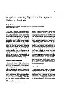
each of them we compare the performance of NB-MPDE with one of the other three algorithms as in Table 3. Comparing NBDE directly with NB-MPDE, the results show that NB-MPDE slightly outperforms NBDE; NB-MPDE achieves significantly better results for 6 data sets, while NBDE achieves significantly better results only for 4 data sets. However, when comparing them with NB, and FTNB, the results clearly show that NB-MPDE achieves significantly better results than both. It achieves significantly better results than NB and FTNB for 23 and 16 data sets, respectively, using the best probability vector of all generations method, while NB achieves significantly better results for only two data set and FTNB achieves only significantly better result for 4 data sets than NB-MPDE (see Table 3). When we compare NB-MPDE with other algorithms based on the number of better results (not just significantly better results), we clearly notice that NB-MPDE wins also in this comparison by achieving better results for at least 30 data sets, while the other algorithms achieve at most 20 better results (see Table 3). Table 4 summarizes NB-MPDE and NBDE experiment results. It shows the differences in average accuracy diff_acc, the number of wins, the number of ties, and the number of losses in (diff_acc/wins/ties/losses) format. Table 4 clearly shows that NB-MPDE outperforms all other algorithms, and that the NBDE also achieves superiority over both FTNB, and NB. Figure 8, summarizes our results using box plots. It shows that NB-MPDE and NBDE methods have higher first quartile, median, and third quartile than NB and FTNB, it also shows that NBMPDE has higher first quartile, median, and third quartile than NBDE. For this reason, we will compare only the NB-MPDE with other remaining algorithms. 99.84

classification accuracy

95

99.68

94.85

85

83.69

75

74.52

99.61

93.98

93.85

82.36

80.88

74.3

72.78

98.86 91.00 80.64

70.22

65 55

54.53

54.84

55.03

45 42.03

35

*36.42

NB-MPDE MPDE

NBDE

FTNB

NB

* Outliers values Fig 8: Box and Whisker plot for classification accuracy of NB, FTNB, NBDE, and NB-MPDE using 53 UCI data sets

18

5.3 Comparing NB-MPDE with Other Metaheuristic based NB Algorithms: In this section, we compare the performance of the NB-MPDE algorithm with the performance of two other metaheuristic-based NB algorithms, namely: Naive Bayes using Genetic Algorithm (NBGA), and Naive Bayes using Simulated Annealing (NBSA). We use the classical version GA, and SA as in described in [26] and reviewed in section 2.4 and 2.5 to find better estimations for the NB used probability terms. The aim is to see which of these three metaheuristic algorithms can find better estimations for the probability terms used by NB, and therefore, gives better NB classification accuracy. To ensure fairness, GA uses the same IPG to create an initial population (see Figure 5), and the same MPDE control parameters values (see section 5.1). SA has similar worst case number of iterations as both GA and MPDE have (i.e. 2500 iterations). SA’s initial high_temperature-value is 500000 and the cooling rate for every iteration is 0.005, while we use population size of 100, and 25 generations for MPDE and GA. The mutation process takes place randomly and proportional to the number of probability terms. SA uses the solution generated by FTNB as an initial solution. It randomly selects the successor of the current solution (see Figure 3, line 7). It creates one successor in every iteration by modifying a small number of current solution values (i.e. conditional probability terms) to create the next solution (see figure 3). The required changes of the current solution should be small and proportional to its size (i.e. the number of the conditional probability terms). We use the ratio (current_solution_size/50) to express the number of needed changes in current solution to create the next solution. The locations for these changes are randomly selected, and assigned by random values in the range [0,1]. We use the final SA, GA, and MPDE solutions to build NBSA, NBGA, and NB-MPDE, respectively, and we conduct several empirical comparisons using NB-MPDE, NBSA, and NBGA. Table 5 shows the detailed results of our experiments. The proposed NB-MPDE achieves 8 significantly better results than NBGA; while NBGA achieves only 3 significantly better result than NB-MPDE. Compared with NBSA, NB-MPDE achieves a significant improvement for 13 data sets, while NBSA achieves only 4 significantly better result than NB-MPDE. When we compare NBGA, and NBSA with NB, each achieves at least 18 significantly better results than NB, while NB achieves at most only 2 significantly better results (when comparing with NBSA). On the other hand, when we compare FTNB, NBGA, and NBSA with each other, their performances are very close. Figure 9 summarizes the results using box plots. It shows that NB-MPDE has higher first quartile, median, and third quartile than all other classifiers. 19

Table 6 shows a comparison between NB, FTNB, NB-MPDE, NBGA, and NBSA in terms of achieving better results (not only significantly better results). NB-MPDE achieves better results for 35, 33, 32 and 35 data sets compared to NB, FTNB, NBGA, and NBSA, respectively, while NBGA, and NBSA achieve at most 19 better results than NB-MPDE. NBGA also achieves 35 better results than NB, while NB achieves only 15 better results than NBGA. On the other hand, NBSA achieves 30 better results than NB, while NB achieves only 19 better results than NBSA. We also compare classifiers with each other according to their execution time. Table 7 shows the average running time in minutes needed for each method to terminate. In general, metaheuristics (i.e. NB-MPDE, NBGA and NBSA) tend to be slow compared to the conventional methods (i.e. NB, and FTNB). Table 7 states clearly that NB-MPDE has the worst average running time of (128.6 min) followed by NBGA of (70.62 min), and finally NBSA comes of (56.14 min). In spite of the difference in the execution time of these classifiers in the training phase, the classification time remains identical for all of them. 110 100 90

91.00

99.61 93.85

80

80.64

80.88

70

70.22

72.27

98.86

99.84 94.85

99.74 93.77

99.61 93.61

83.69

83.19

82.60

74.52

73.90

74.30

60

55.03

50 40

54.53

54.84

54.50

42.03 * 36.42

30 NB * Outliers values

FTNB

NB-MPDE

NB-GA NBGA

NB-SA NBSA

Fig 9: Box and whisker plot for classification accuracy of NB, FTNB, NB-MPDE, NBGA and NBSA using 53 general data sets.

5.4 Using NB-MPDE for Text Classification In this section, we compare the performance of NB-MPDE with two state of the art algorithms for text classification, namely: Bernoulli Naïve Bayes (BNB) and Multinomial Naive Bayes (MNB). In this empirical work, we also use WEKA framework and 18 text classification benchmark data sets obtained from the WEKA web site [75]. (See Table 1(b)) All ordinal attributes were discretized using Fayyad et al.’s [77] supervised discretization method as implemented in WEKA.

20

We used similar control parameters values mentioned in section 5.1), but we use a relatively small population of 10 individuals for 5 generations to minimize the execution time. We conduct several comparisons between NB-MPDE, BNB, MNB, and FTNB using the best probability vector of all generations method. Table 8 shows the detailed results of the experiments. The proposed NB-MPDE achieves significantly better results than BNB and FTNB for 11, and 7 data sets, respectively; on the other hand, neither BNB nor FTNB achieves any significantly better result than NB-MPDE. Moreover, NB-MPDE achieves significantly better results for 5 data sets than MNB, while MNB achieves a significantly better result for only one data set. Table 9 shows the results of BNB, FTNB, MNB, and NB-MPDE in terms achieving better results (not only significantly better results). NB-MPDE achieves better results for 7, 12, and 13 data sets compared to MNB, FTNB, and BNB, respectively, while the other algorithms achieve better results at most for 6 data sets. Figure 10 summarizes the results using box plots. It shows that NB-MPDE has higher first quartile, median, and third quartile than BNB, FTNB, and MNB. We conducted more experiments using different values for population size and generation number, we notice that the bigger the population size and the more generations we use, the better the performance we get. Of course, these better results come on account of training time. For instance, when we increase the population size to 100 and generation number to 25, NB-MPDE achieves significantly better results than FTNB for 10 data sets; and it achieves significantly better results than MNB for 6 data sets and neither FTNB nor MNB achieves any significantly better result than NB-MPDE.

classification accuracy

95

94.91 90.87 88.31

85

94.91

94.91 88.67 83.35

82.38

84.51

82.2 75.50

73.81

65

89.07

87.25

76.17

75

94.92

76.95 73.81

62.5 58.01

55

*50.00

*48.62

45 NB-MPDE

FTNB

*56.90

BNB NB

MNB

* Outliers values Fig 10: Box and whisker plot for classification accuracy of NB, FTNB, MNB, and NB-MPDE using 18 textclassification data sets.

21

6. CONCLUSION: In this paper, we address the issue of finding better estimations for the probability terms used by NB as an optimization problem. We use three different metaheuristic methods to find the required solution, namely, differential evolution, genetic algorithms and simulated annealing, we also propose a novel DE algorithm that uses multi-parent mutation and crossover operations (MPDE). We use the resulted solution of these methods to build NB, and name these new NB classifiers NBDE, NBGE, NBSA, NB-MPDE, respectively. Our empirical results show that DE in general and the proposed MPDE algorithm in particular are more convenient to fine tune NB than all other methods, including the other two metaheuristic methods (GA, and SA), and the proposed MPDE also enhances NB significantly in many domains, especially in text classification where NBMPDE achieves superiority over FTNB, MNB, and BNB methods. Our proposed methods are useful in many domains especially, when the training data are insufficient to reflect the underlying distribution of the instances and give accurate estimations of the required conditional probability terms. The major drawback of using MPDE and other metaheuristic methods in fine-tuning NB classifiers is that they require relatively long training time, but this will not effect on the classification time. Many advanced DE versions have been recently proposed e.g. [79,80], we intend, as a future work, to exploit such improvements to get better results. Our methods can also be used to fine tuning other new versions of NB algorithms such as Hidden Naïve Bayes (HNB)[30], Aggregating One-Dependence Estimators (AODE)[81], and Weighted Average of One-Dependence Estimators (WAODE)[82]. These algorithms relax the independency assumption of NB. We believe that our algorithms will enhance these algorithms significantly. The Selective Fine-Tuning algorithm [83] which was designed to fine tune Bayesian Networks may be used to generate the required initial populations for GA ,SA, DE, and MPDE. Another area for future study is to consider the final solution selection methods as categorical variables which could be tuned for a specific dataset, and try different metrics such as precision, recall, the harmonic mean F score and the ROC curve to evaluate our methods.

Acknowledgment This work was supported by the Research Center of College of Computer and Information Sciences, King Saud University. The authors are grateful for this support.

22

7. REFERENCES: [1]

D.R. Wilson, T.R. Martinez, Improved heterogeneous distance functions, J. Artif. Intell. Res. 6 (1997) 1–34. doi:10.1613/jair.346.

[2]

H. Ragas, C.H.A. Koster, Four text classification algorithms compared on a Dutch corpus, in: Proc. 21st Annu. Int. ACM SIGIR Conf. Res. Dev. Inf. Retr. - SIGIR ’98, ACM Press, New York, New York, USA, 1998: pp. 369–370. doi:10.1145/290941.291059.

[3]

S. Dumais, J. Platt, D. Heckerman, M. Sahami, Inductive learning algorithms and representations for text categorization, in: Proc. Seventh Int. Conf. Inf. Knowl. Manag. CIKM ’98, ACM Press, New York, New York, USA, 1998: pp. 148–155. doi:10.1145/ 288627.288651.

[4]

M. Pazzani, D. Billsus, Learning and Revising User Profiles: The Identification of Interesting Web Sites, Mach. Learn. 27 (1997) 313–331. doi:10.1023/A:1007369909943.

[5]

A. Danesh, B. Moshiri, O. Fatemi, Improve Text Classification Accuracy based on Classifier Fusion Methods, 2007 10th Int. Conf. Inf. Fusion. (2007) 1–6. doi:10.1109/ ICIF.2007.4408196.

[6]

K. Shin, A. Abraham, S.Y. Han, Improving kNN Text Categorization by Removing Outliers from Training Set, in: Springer Berlin Heidelberg, 2006: pp. 563–566. doi:10. 1007/11671299_58.

[7]

M. Mehta, R. Agrawal, J. Rissanen, SLIQ: A Fast Scalable Classifier for Data Mining, Proc. 5th Int. Conf. Extending Database Technol. Adv. Database Technol. (1996) 18–32.

[8]

D.E. Johnson, F.J. Oles, T. Zhang, T. Goetz, A decision-tree-based symbolic rule induction system for text categorization, (n.d.).

[9]

T. Joachims, Text Categorization with Support Vector Machines: Learning with Many Relevant Features, (n.d.).

[10] Chen donghui, Liu zhijing, A new text categorization method based on HMM and SVM, in: 2010 2nd Int. Conf. Comput. Eng. Technol., IEEE, 2010: pp. V7-383-V7-386. doi:10.1109/ICCET.2010.5485482. [11] C.H. Li, S.C. Park, An efficient document classification model using an improved back propagation neural network and singular value decomposition, Expert Syst. Appl. 36 (2009) 3208–3215. doi:10.1016/j.eswa.2008.01.014. [12] A.J.C. Trappey, F.-C. Hsu, C. V Trappey, C.-I. Lin, Development of a patent document classification and search platform using a back-propagation network, (n.d.). doi:10.1016 /j.eswa.2006.01.013. 23

[13] Y. Yang, C.G. Chute, An example-based mapping method for text categorization and retrieval, ACM Trans. Inf. Syst. 12 (1994) 252–277. doi:10.1145/183422.183424. [14] A. Onan, S. Korukoğlu, H. Bulut, A multiobjective weighted voting ensemble classifier based on differential evolution algorithm for text sentiment classification, Expert Syst. Appl. 62 (2016) 1–16. doi:10.1016/j.eswa.2016.06.005. [15] Y.H. Li, A.K. Jain, Classification of Text Documents, Comput. J. 41 (1998) 537–546. doi:10.1093/comjnl/41.8.537. [16] L.S. Larkey, W.B. Croft, Combining classifiers in text categorization, in: Proc. 19th Annu. Int. ACM SIGIR Conf. Res. Dev. Inf. Retr. - SIGIR ’96, ACM Press, New York, New York, USA, 1996: pp. 289–297. doi:10.1145/243199.243276. [17] S.M. Kamruzzaman, C.M. Rahman, Text Categorization using Association Rule and Naive Bayes Classifier, (2010). doi:10.3923/ajit.2004.657.665. [18] S. Buddeewong, W. Kreesuradej, A new association rule-based text classifier algorithm, in: 17th IEEE Int. Conf. Tools with Artif. Intell., IEEE, 2005: p. 2 pp.-pp.685. doi:10.11 09/ICTAI.2005.13. [19] D.D. Lewis, Naive (Bayes) at forty: The independence assumption in information retrieval, in: Springer Berlin Heidelberg, 1998: pp. 4–15. doi:10.1007/BFb0026666. [20] A. McCallum, K. Nigam, A comparison of event models for naive bayes text classification, AAAI-98 Work. Learn. Text. (1998). http://citeseerx.ist.psu.edu/viewdoc/ download?doi=10.1.1.65.9324&rep=rep1&type=pdf (accessed June 7, 2016). [21] W. Medhat, A. Hassan, H. Korashy, Sentiment analysis algorithms and applications: A survey, Ain Shams Eng. J. 5 (2014) 1093–1113. doi:10.1016/j.asej.2014.04.011. [22] G.I. Alkhatib, Agent Technologies and Web Engineering: Applications and Systems ... Google Books, n.d. https://books.google.com.sa/books/about/Agent_Technologies_and Web_Engineering.html?id=MxoRObEY5OUC&source=kp_cover&safe=on&redir_esc=y [23] A. Garg, D. Roth, Understanding Probabilistic Classifiers, (n.d.). [24] X. Wu, V. Kumar, J. Ross Quinlan, J. Ghosh, Q. Yang, H. Motoda, G.J. McLachlan, A. Ng, B. Liu, P.S. Yu, Z.-H. Zhou, M. Steinbach, D.J. Hand, D. Steinberg, Top 10 algorithms in data mining, Knowl. Inf. Syst. 14 (2007) 1–37. doi:10.1007/s10115-007-0114-2. [25] I. Rish, An empirical study of the naive Bayes classifier, IJCAI 2001 Work. Empir. Methods Artif. (2001) 41–46. doi:10.1039/b104835j. [26] S.J. Russell, P. Norvig, A Modern Approach, Artif. Intell. Prentice-Hall, Egnlewood Cliffs. 25 (1995) 27. https://cs.uga.edu/sites/default/files/CIS_CSCI_4550.pdf (accessed June 7, 2016). 24

[27] J.D.M. Rennie, L. Shih, J. Teevan, D.R. Karger, Tackling the Poor Assumptions of Naive Bayes Text Classifiers, (2003). https://www.researchgate.net/publication/228057571 _Tackling_the_Poor_Assumptions_of_Naive_Bayes_Text_Classifiers (accessed June 6, 2016). [28] M. Mitchell, T, Machine learning, MIT Press. (1997) 414. doi:10.1007/978-1-4419-14286. [29] L. Ying, Analysis on Text Classification Using Naive Bayes, Comput. Knowl. Technol. (Academic. (2007). http://en.cnki.com.cn/Article_en/CJFDTOTAL-DNZS200722068 .htm (accessed June 7, 2016). [30] Liangxiao Jiang, H. Zhang, Zhihua Cai, A Novel Bayes Model: Hidden Naive Bayes, IEEE Trans. Knowl. Data Eng. 21 (2009) 1361–1371. doi:10.1109/TKDE.2008.234. [31] H. Zhang, L. Jiang, J. Su, Hidden naive bayes, Proc. Natl. Conf. (2005) 919–924. http://www.aaai.org/Papers/AAAI/2005/AAAI05-145.pdf (accessed October 23, 2016). [32] A. Gupte, S. Joshi, P. Gadgul, A. Kadam, Comparative Study of Classification Algorithms used in Sentiment Analysis, (n.d.). [33] L. Liangxiao Jiang, H. Zhang, Learning Instance Greedily Cloning Naive Bayes for Ranking, in: Fifth IEEE Int. Conf. Data Min., IEEE, 2005: pp. 202–209. doi:10.1109 /ICDM.2005.87. [34] L. Jiang, H. Zhang, J. Su, Instance Cloning Local Naive Bayes, in: 2005: pp. 280–291. doi:10.1007/11424918_29. [35] L. JIANG, D. WANG, H. ZHANG, Z. CAI, B. HUANG, USING INSTANCE CLONING TO IMPROVE NAIVE BAYES FOR RANKING, Int. J. Pattern Recognit. Artif. Intell. 22 (2008) 1121–1140. doi:10.1142/S0218001408006703. [36] K. El Hindi, Fine tuning the Naïve Bayesian learning algorithm, AI Commun. 27 (2014) 133–141. doi:10.3233/AIC-130588. [37] K. El Hindi, A noise tolerant fine tuning algorithm for the Naïve Bayesian learning algorithm, J. King Saud Univ. - Comput. Inf. Sci. 26 (2014) 237–246. doi:10.1016/j.jk suci.2014.03.008. [38] L. Zhang, L. Jiang, C. Li, A New Feature Selection Approach to Naive Bayes Text Classifiers, Int. J. Pattern Recognit. Artif. Intell. 30 (2016) 1650003. doi:10.1142/S0218 001416500038. [39] C.D. Manning, P. Raghavan, An Introduction to Information Retrieval, 2009. doi:10.1109 /LPT.2009.2020494. [40] H. LIANG, J. XU, Y. CHENG, An Improving Text Categorization Method of Naive Bayes, 25

J.

Hebei

Univ.

(Natural.

(2007).

http://en.cnki.com.cn/Article_en/CJFDTotal-

HBDD200703024.htm (accessed June 7, 2016). [41] L. Jiang, Z. Cai, D. Wang, H. Zhang, Improving Tree augmented Naive Bayes for class probability estimation, Knowledge-Based Syst. (2012). http://www.sciencedirect.com /science/article/pii/S0950705111001894 (accessed June 7, 2016). [42] M.E.H. Pedersen, M.E.H. Pedersen, Tuning & Simplifying Heuristical Optimization, (2010). http://citeseerx.ist.psu.edu/viewdoc/summary?doi=10.1.1.216.1838 (accessed June 7, 2016). [43] R. Storn, K. Price, Differential Evolution – A Simple and Efficient Heuristic for global Optimization over Continuous Spaces, J. Glob. Optim. 11 (1997) 341–359. doi:10.1023 /A:1008202821328. [44] R. Gämperle, S. Müller, A parameter study for differential evolution, Adv. Intell. (2002). http://natcomp.liacs.nl/SWI/papers/Differential

Evolution/A

Parameter

Study

for

Differential Evolution.pdf (accessed June 7, 2016). [45] J. Wu, Z. Cai, Attribute weighting via differential evolution algorithm for attribute weighted naive bayes (wnb), J. Comput. Inf. Syst. 2011. (n.d.). https://www.researchgate .net/profile/Jia_Wu12/publication/266464512_Attribute_Weighting_via_Differential_Ev olution_Algorithm_for_Attribute_Weighted_Naive_Bayes_(WNB)/links/55209adb0cf2f9 c13050c4da.pdf (accessed June 6, 2016). [46] A.H. Wright, Genetic algorithms for real parameter optimization, Found. Genet. Agorithms. (1990) 205–220. doi:citeulike-article-id:1439583. [47] S.M. Elsayed, R.A. Sarker, D.L. Essam, A new genetic algorithm for solving optimization problems, Eng. Appl. Artif. Intell. 27 (2014) 57–69. doi:10.1016/ j.engappai.2013.09.013. [48] L. Zhang, L. Jiang, C. Li, G. Kong, Two feature weighting approaches for naive Bayes text classifiers, Knowledge-Based Syst. 100 (2016) 137–144. doi:10.1016/j.knosys. [49] L. Jiang, C. Li, S. Wang, L. Zhang, Deep feature weighting for naive Bayes and its application to text classification, Eng. Appl. Artif. Intell. 52 (2016) 26–39. doi:10.1016/j.engappai.2016.02.002. [50] S. Taheri, M. Mammadov, A.M. Bagirov, Improving Naive Bayes Classifier Using Conditional Probabilities, (2010) 63–68. http://dl.acm.org/citation.cfm?id=2483628 .2483637 (accessed June 6, 2016). [51] C. Qiu, L. Jiang, C. Li, Not always simple classification: Learning SuperParent for class probability estimation, Expert Syst. Appl. 42 (2015) 5433–5440. doi:10.1016/j.eswa. 26

2015.02.049. [52] L. Jiang, S. Wang, C. Li, L. Zhang, Structure extended multinomial naive Bayes, Inf. Sci. (Ny). 329 (2016) 346–356. doi:10.1016/j.ins.2015.09.037. [53] J. Wu, S. Pan, X. Zhu, P. Zhang, C. Zhang, SODE: Self-Adaptive One-Dependence Estimators for classification, Pattern Recognit. 51 (2016) 358–377. doi:10.1016/ j.patcog.2015.08.023. [54] L. Jiang, H. Zhang, Z. Cai, J. Su, Evolutional naive bayes, Proc. 1st Int. Symp. …. (2005). https://scholar.google.com/scholar?cluster=18248474948955544657&hl=en&oi= scholarr#0 (accessed June 6, 2016). [55] L. Jiang, D. Wang, Z. Cai, Discriminatively Weighted Naive Bayes and its Application in Text

Classification,

Int.

J.

Artif.

Intell.

Tools.

21

(2012)

1250007.

doi:10.1142/S0218213011004770. [56] Judea Pearl, Probabilistic reasoning in intelligent systems: Networks of plausible inference, Morgan Kaufmann Publishers, 1991. doi:10.1016/0020-7101(91)90056-K. [57] N. Friedman, D. Geiger, M. Goldszmidt, Bayesian Network Classifiers, Mach. Learn. 29 (1997) 131–163. doi:10.1023/A:1007465528199. [58] H. Zhang, C. Ling, An improved learning algorithm for augmented naive Bayes, Adv. Knowl. Discov. Data Min. (2001). http://link.springer.com/chapter/10.1007/3-540-453571_62 (accessed June 7, 2016). [59] P. Langley, S. Sage, Induction of Selective Bayesian Classifiers, Proc. Tenth Int. Conf. Uncertain. Artif. Intell. (1994) 399–406. http://dl.acm.org/citation.cfm?id=2074445 (accessed June 7, 2016). [60] M.A. Palacios-Alonso, C.A. Brizuela, L.E. Sucar, Evolutionary Learning of Dynamic Naive Bayesian Classifiers, J. Autom. Reason. 45 (2009) 21–37. doi:10.1007/s10817-0099130-0. [61] L. Jiang, Z. Cai, H. Zhang, D. Wang, Not so greedy: Randomly Selected Naive Bayes, Expert Syst. Appl. 39 (2012) 11022–11028. doi:10.1016/j.eswa.2012.03.022. [62] M. Hall, A decision tree-based attribute weighting filter for naive Bayes, Knowledge-Based Syst. 20 (2007) 120–126. doi:10.1016/j.knosys.2006.11.008. [63] J. Vesterstrom, R. Thomsen, A comparative study of differential evolution, particle swarm optimization, and evolutionary algorithms on numerical benchmark problems, in: Proc. 2004 Congr. Evol. Comput. (IEEE Cat. No.04TH8753), IEEE, 2004: pp. 1980–1987. doi:10.1109/CEC.2004.1331139. [64] R. Storn, System design by constraint adaptation and differential evolution, IEEE Trans. 27

Evol. Comput. 3 (1999) 22–34. doi:10.1109/4235.752918. [65] R. Thomsen, Flexible ligand docking using differential evolution, in: 2003 Congr. Evol. Comput. CEC 2003 - Proc., IEEE, 2003: pp. 2354–2361. doi:10.1109/CEC.2003. 1299382. [66] M.M. Ali, A. Törn, Population set-based global optimization algorithms: some modifications and numerical studies, Comput. Oper. Res. 31 (2004) 1703–1725. doi:10.1016/S0305-0548(03)00116-3. [67] K. Price, R. Storn, J. Lampinen, Differential evolution: a practical approach to global optimization, (2005). http://dl.acm.org/citation.cfm?id=1121631 (accessed June 6, 2016). [68] Alan C. Bovik, A.C. Bovik, Document Clustering Using Differential Evolution, Optimization. 38 (2008) 1–38. doi:10.1109/CEC.2006.1688523. [69] H. Zhou, Q. Zhang, H. Wang, D. Zhang, Feature selection in medical text classification based on Differential Evolution Algorithm, in: Electron. Inf. Technol. Intellectualization, CRC Press, 2015: pp. 79–82. doi:10.1201/b17988-20. [70] Y. Ao, H. Chi, Multi-parent mutation in differential evolution for multi-objective optimization, in: 5th Int. Conf. Nat. Comput. ICNC 2009, IEEE, 2009: pp. 618–622. doi:10.1109/ICNC.2009.149. [71] S. Tsutsui, M. Yamamura, T. Higuchi, Multi-parent recombination with simplex crossover in real coded genetic algorithms, Proc. 1999 Genet. Evol. Comput. Conf. (1999) 657–664. http://www2.hannan-u.ac.jp/~tsutsui/ps/icga99.pdf (accessed June 7, 2016). [72] G. Liu, Y. Li, X. Nie, H. Zheng, A novel clustering-based differential evolution with 2 multi-parent crossovers for global optimization, Appl. Soft Comput. (2012). http://www.sciencedirect.com/science/article/pii/S1568494611004212 (accessed June 7, 2016). [73] Z. Yang, K. Tang, X. Yao, Differential evolution for high-dimensional function optimization, in: 2007 IEEE Congr. Evol. Comput. CEC 2007, IEEE, 2007: pp. 3523–3530. doi:10.1109/CEC.2007.4424929. [74] Z. Yang, K. Tang, X. Yao, Self-adaptive differential evolution with neighborhood search, in: 2008 IEEE Congr. Evol. Comput. CEC 2008, IEEE, 2008: pp. 1110–1116. doi:10.1109/CEC.2008.4630935. [75] I.H. Witten, E. Frank, Data Mining: Practical Machine Learning Tools and Techniques, Second Edition, 2005. https://books.google.com/books?hl=en&lr=&id=QTnOcZJzlUoC &pgis=1 (accessed June 6, 2016). [76] C.L. Blake, C.J. Merz, UCI Repository of machine learning databases, Univ. Calif. (1998) 28

http://archive.ics.uci.edu/ml/. http://archive.ics.uci.edu/ml/ (accessed March 12, 2015). [77] U.M. Fayyad, K.B. Irani, Multi-Interval Discretization of Continuos-Valued Attributes for Classification Learning, in: Proc. Int. Jt. Conf. Uncertain. AI, Proceedings of the International Joint Conference on Uncertainty in AI, 1993: pp. 1022–1027. http://trsnew.jpl.nasa.gov/dspace/handle/2014/35171 (accessed June 7, 2016). [78] S.M. Islam, S. Das, S. Ghosh, S. Roy, P.N. Suganthan, An Adaptive Differential Evolution Algorithm With Novel Mutation and Crossover Strategies for Global Numerical Optimization, IEEE Trans. Syst. Man, Cybern. Part B. 42 (2012) 482–500. doi:10.1109/TSMCB.2011.2167966. [79] Z. Dai, A. Zhou, G. Zhang, S. Jiang, A differential evolution with an orthogonal local search, in: 2013 IEEE Congr. Evol. Comput. CEC 2013, 2013: pp. 2329–2336. doi:10.1109/CEC.2013.6557847. [80] W. Gong, Z. Cai, L. Jiang, Enhancing the performance of differential evolution using orthogonal design method, Appl. Math. Comput. (2008). http://www.sciencedirect.com /science/article/pii/S0096300308006280 (accessed June 7, 2016). [81] G.I. Webb, J.R. Boughton, Z. Wang, Not so naive Bayes: Aggregating one-dependence estimators, Mach. Learn. 58 (2005) 5–24. doi:10.1007/s10994-005-4258-6. [82] L. Jiang, H. Zhang, Z. Cai, D. Wang, Weighted average of one-dependence estimators†, J. Exp. Theor. Artif. Intell. 24 (2012) 219–230. doi:10.1080/0952813X.2011.639092. [83] A. Alhussan, K. El Hindi, Selectively Fine-Tuning Bayesian Network Learning Algorithm, Int. J. Pattern Recognit. Artif. Intell. 30 (2016) 1651005. doi:10.1142/S0218001416510058

29

APPENDIX. ADDITIONAL DETAILS OF STATISTICAL COMPARISONS Table 1: General UCI and Text UCI Data sets a) General UCI Data sets Data Set breast-w heart-statlog Hypothyroid Ionosphere Iris Zoo Waveform-5000 Sick Segment lung-cancer liver-disorders Hepatitis heart-h heart-c Haberman Flags Diabetes cylinder-bands credit-g credit-a bridges_version2 bridges_version1 colic.orig Colic Autos Car breast-cancer

Inst 699 270 3772 351 150 101 5000 3772 2310 32 345 155 294 303 306 194 768 512 690 1000 108 108 368 368 205 1728 286

Class 2 2 4 2 3 7 3 2 7 3 2 2 5 5 2 8 2 2 2 2 6 6 2 2 7 4 2

Atts 10 14 30 35 5 18 41 30 20 57 8 20 14 14 4 31 9 40 16 21 13 13 28 23 26 7 10

Miss Y N Y N N N N Y N Y N Y Y Y N N N Y Y Y Y Y Y Y Y N Y

Name Anneal Vote Vehicle Trains Nursery optdigits pendigits Lymph Sonar wine Modified anneal.ORIG Dermatology solar-flare_1 solar-flare_2 spam base Soybean Vowel balance-scale Audiology kr-vs-kp Glass Ecoli Mushroom Letter Splice Arrhythmia

b) Text UCI Data sets Inst 898 435 846 10 12960 5620 10992 148 208 178 898 366 1066 1066 4601 683 990 625 226 3196 214 363 8124 20000 3190 452

Class 6 2 4 2 5 10 10 4 2 3 6 6 6 6 2 19 11 3 24 2 7 8 2 26 3 16

Atts 39 17 19 33 9 65 17 19 61 14 39 34 13 13 58 36 14 5 70 37 10 9 23 17 62 280

Miss Y Y N Y N N N N N N Y Y N N N Y N N Y N N N Y N N Y

Data Set tr12 tr11 tr21 tr23 tr31 tr41 tr45 oh0 fbis1 Wap la1s la2s oh5 oh15 re0 oh10 re1 ohscal

Inst 313 414 336 204 927 878 690 1003 463 1561 3204 3075 918 914 1504 1050 1658 11163

Class 8 9 6 6 7 10 10 10 17 20 6 6 10 10 13 10 25 10

Atts 5805 6430 7903 5833 10129 7455 8262 3183 2001 8461 13196 12433 3013 3101 2887 3239 3759 11466

30

Miss N N N N N N N N N N N N N N N N N N

Table 2: Comparing number of significantly better results between three methods NB, FTNB, and NBDE using 53 general domain UCI datasets and three methods to find the final solution when DE reaches the maximum number of generations.

Best probability vector of all generations

Data Set 1 2 3 4 5 6 7 8 9 10 11 12 13 14 15 16 17 18 19 20 21 22 23 24 25 26 27 28 29 30 31 32

breast-w heart-statlog Hypothyroid Ionosphere Iris Zoo Waveform-5000 Sick Segment lung-cancer liver-disorders Hepatitis heart-h heart-c Haberman Flags Diabetes cylinder-bands credit-g credit-a bridges_version2 bridges_version1 colic.orig Colic Autos Car breast-cancer Anneal Vote Vehicle Trains Nursery

Average of best solutions of all generations

Best averages of the solutions of each generation

NB %

FTNB %

NBDE %

NB %

NBDE %

FTNB %

NB %

FTNB %

NBDE %

NB %

NBDE %

FTNB %

NB %

FTNB %

NBDE %

NB %

NBDE %

FTNB %

97.28 83.70 92.95 90.88 95.33 91.00 80.64 96.85 91.77 80.00 54.84 83.00 83.21 85.20 74.19 60.13 77.34 69.44 75.50 84.06 57.64 59.00 70.65 72.02 59.95 73.14 73.13 97.00 89.43 63.36 70.00 81.37

96.14 83.33 99.26 92.29 95.33 91.00 83.94 96.79 93.85 76.67 63.22 87.63 79.92 83.86 70.95 55.03 77.08 71.30 74.10 82.03 58.64 60.09 75.51 80.71 62.86 80.96 67.86 97.55 93.09 67.84 70.00 85.00

96.43 84.44 99.31 92.01 95.33 91.00 84.14 97.22 93.98 76.67 54.84 87.00 80.52 84.18 73.51 58.13 78.52 73.52 74.30 81.74 58.64 60.00 74.15 82.34 62.88 80.84 70.30 98.33 93.78 68.55 70.00 87.19

97.28 83.70 92.95 90.88 95.33 91.00 80.64 96.85 91.77 80.00 54.84 83.00 83.21 85.20 74.19 60.13 77.34 69.44 75.50 84.06 57.64 59.00 70.65 72.02 59.95 73.14 73.13 97.00 89.43 63.36 70.00 81.37

96.43 84.44 99.31 92.01 95.33 91.00 84.14 97.22 93.98 76.67 54.84 87.00 80.52 84.18 73.51 58.13 78.52 73.52 74.30 81.74 58.64 60.00 74.15 82.34 62.88 80.84 70.30 98.33 93.78 68.55 70.00 87.19

96.14 83.33 99.26 92.29 95.33 91.00 83.94 96.79 93.85 76.67 63.22 87.63 79.92 83.86 70.95 55.03 77.08 71.30 74.10 82.03 58.64 60.09 75.51 80.71 62.86 80.96 67.86 97.55 93.09 67.84 70.00 85.00

97.28 83.70 92.95 90.88 95.33 91.00 80.64 96.85 91.78 80.00 54.84 83.00 83.21 85.20 74.19 60.13 77.33 69.44 75.50 84.06 57.64 59.00 70.65 72.02 59.95 73.14 73.13 97.00 89.43 63.36 70.00 81.37

96.14 83.33 99.26 92.29 95.33 91.00 83.94 96.79 93.85 76.67 63.22 87.63 79.92 83.86 70.95 55.03 77.08 71.30 74.10 82.03 58.64 60.09 75.51 80.71 62.86 80.96 67.86 97.55 93.09 67.84 70.00 85.00

96.57 83.33 99.34 92.01 96.00 91.00 84.42 97.11 94.16 76.67 54.84 87.67 80.85 83.19 73.86 57.63 77.87 72.04 75.30 81.02 59.46 59.18 74.14 82.35 62.86 83.56 68.89 98.11 93.55 67.37 70.00 86.57

97.28 83.70 92.95 90.88 95.33 91.00 80.64 96.85 91.78 80.00 54.84 83.00 83.21 85.20 74.19 60.13 77.33 69.44 75.50 84.06 57.64 59.00 70.65 72.02 59.95 73.14 73.13 97.00 89.43 63.36 70.00 81.37

96.57 83.33 99.34 92.01 96.00 91.00 84.42 97.11 94.16 76.67 54.84 87.67 80.85 83.19 73.86 57.63 77.87 72.04 75.30 81.02 59.46 59.18 74.14 82.35 62.86 83.56 68.89 98.11 93.55 67.37 70.00 86.57

96.14 83.33 99.26 92.29 95.33 91.00 83.94 96.79 93.85 76.67 63.22 87.63 79.92 83.86 70.95 55.03 77.08 71.30 74.10 82.03 58.64 60.09 75.51 80.71 62.86 80.96 67.86 97.55 93.09 67.84 70.00 85.00

97.28 83.70 92.95 90.88 95.33 91.00 80.64 96.85 91.78 80.00 54.84 83.00 83.21 85.20 74.19 60.13 77.34 69.44 75.50 84.06 57.64 59.00 70.65 72.02 59.95 73.13 73.13 97.00 89.43 63.36 70.00 81.37

96.14 83.33 99.26 92.29 95.33 91.00 83.94 96.79 93.85 76.67 63.22 87.63 79.92 83.86 70.95 55.03 77.08 71.30 74.10 82.03 58.64 60.09 75.51 80.71 62.86 80.96 67.86 97.55 93.09 67.84 70.00 85.00

96.43 82.96 99.39 92.01 95.33 91.00 84.46 97.14 94.33 76.67 54.84 87.00 82.20 82.87 73.86 57.11 77.60 72.41 74.90 80.73 60.36 60.09 74.70 82.62 62.86 82.52 69.95 98.11 94.00 67.72 70.00 86.70

97.28 83.70 92.95 90.88 95.33 91.00 80.64 96.85 91.78 80.00 54.84 83.00 83.21 85.20 74.19 60.13 77.34 69.44 75.50 84.06 57.64 59.00 70.65 72.02 59.95 73.13 73.13 97.00 89.43 63.36 70.00 81.37

96.43 82.96 99.39 92.01 95.33 91.00 84.46 97.14 94.33 76.67 54.84 87.00 82.20 82.87 73.86 57.11 77.60 72.41 74.90 80.73 60.36 60.09 74.70 82.62 62.86 82.52 69.95 98.11 94.00 67.72 70.00 86.70

96.14 83.33 99.26 92.29 95.33 91.00 83.94 96.79 93.85 76.67 63.22 87.63 79.92 83.86 70.95 55.03 77.08 71.30 74.10 82.03 58.64 60.09 75.51 80.71 62.86 80.96 67.86 97.55 93.09 67.84 70.00 85.00

31

Best probability vector of all generations

33 34 35 36 37 38 39 40 41 42 43 44 45 46 47 48 49 50 51 52 53

Best averages of the solutions of each generation

Data Set

NB %

FTNB %

NBDE %

NB %

NBDE %

FTNB %

NB %

FTNB %

NBDE %

NB %

NBDE %

FTNB %

NB %

FTNB %

NBDE %

NB %

NBDE %

FTNB %

opt digits pen digits Lymph Sonar wine Modified anneal.ORIG Dermatology solar-flare_1 solar-flare_2 spam base Soybean Vowel balance-scale Audiology kr-vs-kp Glass Ecoli Mushroom Letter Splice Arrhythmia

92.12 87.92 83.81 82.36 98.86 79.07 97.27 91.62 97.00 89.35 42.03 61.31 77.57 36.42 66.57 70.22 74.16 94.33 74.11 94.92 54.22 78.48

93.93 94.65 85.81 79.52 98.86 97.11 97.28 95.97 98.87 80.88 72.42 62.53 79.99 61.58 76.46 74.35 77.21 99.61 77.16 93.01 72.78 81.58

94.07 94.72 83.81 82.36 98.86 98.00 97.55 95.96 98.87 89.85 77.26 61.62 77.09 65.13 86.11 76.30 76.92 99.68 77.89 93.42 75.44 82.35

92.12 87.92 83.81 82.36 98.86 79.07 97.27 91.62 97.00 89.35 42.03 61.31 77.57 36.42 66.57 70.22 74.16 94.33 74.11 94.92 54.22 78.48

94.07 94.72 83.81 82.36 98.86 98.00 97.55 95.96 98.87 89.85 77.26 61.62 77.09 65.13 86.11 76.30 76.92 99.68 77.89 93.42 75.44 82.35

93.93 94.65 85.81 79.52 98.86 97.11 97.28 95.97 98.87 80.88 72.42 62.53 79.99 61.58 76.46 74.35 77.21 99.61 77.16 93.01 72.78 81.58

92.12 87.92 83.81 82.36 98.86 79.07 97.28 91.62 97.00 89.35 42.03 61.31 77.57 36.42 66.57 70.22 74.16 94.33 74.11 94.92 54.22 78.48

93.93 94.65 85.81 79.52 98.86 97.11 97.28 95.97 98.87 80.88 72.42 62.53 79.99 61.58 76.46 74.35 77.21 99.61 77.16 93.01 72.78 81.58

94.13 94.65 85.81 81.36 98.86 98.00 97.82 95.97 98.87 87.40 74.62 61.92 77.25 62.02 84.02 76.75 78.73 99.73 77.70 93.04 75.89 82.18

92.12 87.92 83.81 82.36 98.86 79.07 97.28 91.62 97.00 89.35 42.03 61.31 77.57 36.42 66.57 70.22 74.16 94.33 74.11 94.92 54.22 78.48

94.13 94.65 85.81 81.36 98.86 98.00 97.82 95.97 98.87 87.40 74.62 61.92 77.25 62.02 84.02 76.75 78.73 99.73 77.70 93.04 75.89 82.18

93.93 94.65 85.81 79.52 98.86 97.11 97.28 95.97 98.87 80.88 72.42 62.53 79.99 61.58 76.46 74.35 77.21 99.61 77.16 93.01 72.78 81.58

92.12 87.92 83.81 82.36 98.86 79.07 97.27 91.62 97.00 89.35 42.03 61.31 77.57 36.42 66.57 70.22 74.16 94.33 74.11 94.92 54.22 78.48

93.93 94.65 85.81 79.52 98.86 97.11 97.27 95.97 98.87 80.88 72.42 62.53 79.99 61.58 76.46 74.35 77.21 99.61 77.16 93.01 72.78 81.58

94.09 94.80 86.48 81.36 98.86 98.00 97.55 96.58 98.87 89.57 75.06 61.82 77.09 64.25 84.62 76.28 79.32 99.72 78.02 93.51 75.00 82.33

92.12 87.92 83.81 82.36 98.86 79.07 97.27 91.62 97.00 89.35 42.03 61.31 77.57 36.42 66.57 70.22 74.16 94.33 74.11 94.92 54.22 78.48

94.09 94.80 86.48 81.36 98.86 98.00 97.55 96.58 98.87 89.57 75.06 61.82 77.09 64.25 84.62 76.28 79.32 99.72 78.02 93.51 75.00 82.33

93.93 94.65 85.81 79.52 98.86 97.11 97.27 95.97 98.87 80.88 72.42 62.53 79.99 61.58 76.46 74.35 77.21 99.61 77.16 93.01 72.78 81.58

15 1

33 18

35 22

11 0

34 7

12 0

15 1

33 18

35 19

14 1

34 6

9 0

15 1

33 18

35 20

13 0

35 7

10 0

Average Accuracy Better Result significantly better results

 

Average of best solutions of all generations

The significant better results are bolded and highlighted

32

Table 3: Comparing number of significantly better results between three methods NB, FTNB, NBDE, and NB-MPDE using best vector of all Generations and 53 general domain UCI datasets

Data Set 1 2 3 4 5 6 7 8 9 10 11 12 13 14 15 16 17 18 19 20 21 22 23 24 25 26 27 28 29 30 31 32 33 34 35 36 37 38 39 40 41 42 43 44 45 46 47 48 49 50 51 52 53

breast-w heart-statlog Hypothyroid Ionosphere Iris Zoo Waveform-5000 Sick Segment lung-cancer liver-disorders Hepatitis heart-h heart-c Haberman Flags Diabetes cylinder-bands credit-g credit-a bridges_version2 bridges_version1 colic.orig Colic Autos Car breast-cancer Anneal Vote Vehicle Trains Nursery opt digits pen digits Lymph Sonar wine Modified anneal.ORIG Dermatology solar-flare_1 solar-flare_2 spam base Soybean Vowel balance-scale Audiology kr-vs-kp Glass Ecoli Mushroom Letter Splice Arrhythmia

Average accuracy Better Results significantly better results



Best vector of all generations NB-MPDE %

NB %

NB-MPDE %

NBDE %

NB-MPDE %

FTNB %

96.43 84.82 99.44 92.02 96.01 95.04 82.44 97.46 94.85 66.67 54.84 86.96 81.52 84.50 77.57 54.53 77.34 71.85 73.50 82.32 57.73 56.36 74.99 83.69 61.38 77.37 71.69 98.22 96.32 69.14 70.00 88.10 91.73 90.10 85.10 74.52 98.30 98.44 98.09 97.52 98.97 94.70 87.46 55.35 77.41 66.46 93.27 76.28 79.60 99.84 77.58 93.45 75.22 82.35 35 23

97.28 83.70 92.95 90.88 95.33 91.00 80.64 96.85 91.77 80.00 54.84 83.00 83.21 85.20 74.19 60.13 77.34 69.44 75.50 84.06 57.64 59.00 70.65 72.02 59.95 73.14 73.13 97.00 89.43 63.36 70.00 81.37 92.12 87.92 83.81 82.36 98.86 79.07 97.27 91.62 97.00 89.35 42.03 61.31 77.57 36.42 66.57 70.22 74.16 94.33 74.11 94.92 54.22 78.48 15 2

96.43 84.82 99.44 92.02 96.01 95.04 82.44 97.46 94.85 66.67 54.84 86.96 81.52 84.50 77.57 54.53 77.34 71.85 73.50 82.32 57.73 56.36 74.99 83.69 61.38 77.37 71.69 98.22 96.32 69.14 70.00 88.10 91.73 90.10 85.10 74.52 98.30 98.44 98.09 97.52 98.97 94.70 87.46 55.35 77.41 66.46 93.27 76.28 79.60 99.84 77.58 93.45 75.22 82.35 30 6

96.43 84.44 99.31 92.01 95.33 91.00 84.14 97.22 93.98 80.00 54.84 87.00 80.52 84.18 73.51 58.13 78.52 73.52 74.30 81.74 58.64 60.00 74.15 82.34 62.88 80.84 70.30 98.33 93.78 68.55 70.00 87.19 94.07 94.72 83.81 82.36 98.86 98.00 97.55 95.96 98.87 89.85 77.26 61.62 77.09 65.13 86.11 76.30 76.92 99.68 77.89 93.42 75.44 82.35 20 4

96.43 84.82 99.44 92.02 96.01 95.04 82.44 97.46 94.85 66.67 54.84 86.96 81.52 84.50 77.57 54.53 77.34 71.85 73.50 82.32 57.73 56.36 74.99 83.69 61.38 77.37 71.69 98.22 96.32 69.14 70.00 88.10 91.73 90.10 85.10 74.52 98.30 98.44 98.09 97.52 98.97 94.70 87.46 55.35 77.41 66.46 93.27 76.28 79.60 99.84 77.58 93.45 75.22 82.35 33 16

96.14 83.33 99.26 92.29 95.33 91.00 83.94 96.79 93.85 76.67 63.22 87.63 79.92 83.86 70.95 55.03 77.08 71.30 74.10 82.03 58.64 60.09 75.51 80.71 62.86 80.96 67.86 97.55 93.09 67.84 70.00 85.00 93.93 94.66 85.81 79.52 98.86 97.11 97.28 95.97 98.87 80.88 72.42 62.53 79.99 61.58 76.46 74.35 77.21 99.61 77.16 93.01 72.78 81.58 19 4

The significant better results are bolded and highlighted

33

Table 4: Comparing NB, FTNB, NBDE, and NB-MPDE using 53 UCI data sets (Better results not only significantly better) Algorithm

Average Accuracy

𝐍𝐁𝐃𝐄𝐁𝐞𝐬𝐭 𝐨𝐟 𝐄𝐧𝐭𝐢𝐫𝐞 𝐆𝐞𝐧𝐞𝐫𝐚𝐭𝐢𝐨𝐧𝐬

NB

FTNB

Diff_Acc/Wins/Ties/losses

Diff_Acc/Wins/Ties/losses

Diff_Acc/Wins/Ties/losses

-

-3.1/15/5/33

-3.87/11/7/35

NB

78.48

FTNB

81.58

+3.1/33/5/15

-

-0.77/12/7/34

NBDE𝐵𝑒𝑠𝑡 𝑜𝑓

82.35

+3.87/35/7/11

+0.77/34/7/12

-

NBDE 𝐴𝑣𝑒𝑟𝑎𝑔𝑒𝑠 𝑜𝑓 𝐵𝑒𝑠𝑡𝑠

82.18

+3.67/35/4/14

+0.57/34/10/9

-0.17/22/8/23

NBDE𝐵𝑒𝑠𝑡 𝑜𝑓

82.33

+3.85/35/5/13

+0.75/35/8/10

-0.02/22/13/18

82.35

+3.87/35/3/15

+0.77/33/1/19

0/30/3/20

𝐸𝑛𝑡𝑖𝑟𝑒 𝑔𝑒𝑛𝑒𝑟𝑎𝑡𝑖𝑜𝑛𝑠

𝐴𝑣𝑒𝑟𝑎𝑔𝑒𝑠

NB-MPDE

Table 5: Comparing number of significantly better results between three methods NB, FTNB, NB-MPDE, NBSA, and NBGA using 53 general domain UCI datasets

Genetic Algorithm

1 2 3 4 5 6 7 8 9 10 11 12 13 14 15 16 17 18 19

Simulated Annealing

Data Set

NBGA %

NB %

NBGA %

FTNB %

NBGA %

NB-MPDE %

NBGA %

NBSA %

NBSA %

NB %

NBSA %

FTNB %

NBSA %

NB-MPDE %

breast-w heart-statlog Hypothyroid Ionosphere Iris Zoo Waveform-5000 Sick Segment lung-cancer liver-disorders Hepatitis heart-h heart-c Haberman Flags Diabetes cylinder-bands credit-g

96.29 84.81 99.23 92.01 94.67 92.00 83.80 96.77 93.77 76.67 54.84 83.71 80.20 83.83 73.86 55.53 77.86 71.11 73.90

97.28 83.70 92.95 90.88 95.33 91.00 80.64 96.85 91.77 80.00 54.84 83.00 83.21 85.20 74.19 60.13 77.34 69.44 75.50

96.29 84.81 99.23 92.01 94.67 92.00 83.80 96.77 93.77 76.67 54.84 83.71 80.20 83.83 73.86 55.53 77.86 71.11 73.90

96.14 83.33 99.26 92.29 95.33 91.00 83.94 96.79 93.85 76.67 63.22 87.63 79.92 83.86 70.95 55.03 77.08 71.30 74.10

96.29 84.81 99.23 92.01 94.67 92.00 83.80 96.77 93.77 76.67 54.84 83.71 80.20 83.83 73.86 55.53 77.86 71.11 73.90

96.43 84.82 99.44 92.02 96.01 95.04 82.44 97.46 94.85 66.67 54.84 86.96 81.52 84.50 77.57 54.53 77.34 71.85 73.50

96.29 84.81 99.23 92.01 94.67 92.00 83.80 96.77 93.77 76.67 54.84 83.71 80.20 83.83 73.86 55.53 77.86 71.11 73.90

96.00 83.33 99.26 91.72 95.33 89.00 83.94 96.74 93.85 83.33 63.22 87.00 77.16 83.86 70.95 54.50 77.08 71.30 74.30

96.00 83.33 99.26 91.72 95.33 89.00 83.94 96.74 93.85 83.33 63.22 87.00 77.16 83.86 70.95 54.50 77.08 71.30 74.30

97.28 83.70 92.95 90.88 95.33 91.00 80.64 96.85 91.77 80.00 54.84 83.00 83.21 85.20 74.19 60.13 77.34 69.44 75.50

96.00 83.33 99.26 91.72 95.33 89.00 83.94 96.74 93.85 83.33 63.22 87.00 77.16 83.86 70.95 54.50 77.08 71.30 74.30

96.14 83.33 99.26 92.29 95.33 91.00 83.94 96.79 93.85 76.67 63.22 87.63 79.92 83.86 70.95 55.03 77.08 71.30 74.10

96.00 83.33 99.26 91.72 95.33 89.00 83.94 96.74 93.85 83.33 63.22 87.00 77.16 83.86 70.95 54.50 77.08 71.30 74.30

96.43 84.82 99.44 92.02 96.01 95.04 82.44 97.46 94.85 66.67 54.84 86.96 81.52 84.50 77.57 54.53 77.34 71.85 73.50

34

Genetic Algorithm Data Set 20

credit-a bridges_version2 bridges_version1 colic.orig Colic Autos Car breast-cancer Anneal Vote Vehicle Trains Nursery Optdigits Pendigits Lymph Sonar wine Modified anneal.ORIG Dermatology solar-flare_1 solar-flare_2 spam base Soybean Vowel balance-scale Audiology kr-vs-kp Glass Ecoli Mushroom Letter Splice Arrhythmia

21 22 23 24 25 26 27 28 29 30 31 32 33 34 35 36 37 38 39 40 41 42 43 44 45 46 47 48 49 50 51 52 53

Average accuracy Better Results significantly better results



Simulated Annealing

NBGA %

NB %

NBGA %

FTNB %

NBGA %

NB-MPDE %

NBGA %

NBSA %

NBSA %

NB %

NBSA %

FTNB %

NBSA %

NB-MPDE %

83.19 61.18 59.27 74.95 81.52 62.33 80.90 66.12 97.77 93.09 67.72 70.00 84.81 93.97 94.41 84.43 80.36 98.86 97.89 98.35 96.28 99.06 90.81 73.44 60.51 76.62 63.34 83.43 75.32 80.48 99.74 77.13 92.85 77.78 81.94

84.06 57.64 59.00 70.65 72.02 59.95 73.14 73.13 97.00 89.43 63.36 70.00 81.37 92.12 87.92 83.81 82.36 98.86 79.07 97.27 91.62 97.00 89.35 42.03 61.31 77.57 36.42 66.57 70.22 74.16 94.33 74.11 94.92 54.22 78.48

83.19 61.18 59.27 74.95 81.52 62.33 80.90 66.12 97.77 93.09 67.72 70.00 84.81 93.97 94.41 84.43 80.36 98.86 97.89 98.35 96.28 99.06 90.81 73.44 60.51 76.62 63.34 83.43 75.32 80.48 99.74 77.13 92.85 77.78 81.94

82.03 58.64 60.09 75.51 80.71 62.86 80.96 67.86 97.55 93.09 67.84 70.00 85.00 93.93 94.66 85.81 79.52 98.86 97.11 97.28 95.97 98.87 80.88 72.42 62.53 79.99 61.58 76.46 74.35 77.21 99.61 77.16 93.01 72.78 81.58

83.19 61.18 59.27 74.95 81.52 62.33 80.90 66.12 97.77 93.09 67.72 70.00 84.81 93.97 94.41 84.43 80.36 98.86 97.89 98.35 96.28 99.06 90.81 73.44 60.51 76.62 63.34 83.43 75.32 80.48 99.74 77.13 92.85 77.78 81.94

82.32 57.73 56.36 74.99 83.69 61.38 77.37 71.69 98.22 96.32 69.14 70.00 88.10 91.73 90.10 85.10 74.52 98.30 98.44 98.09 97.52 98.97 94.70 87.46 55.35 77.41 66.46 93.27 76.28 79.60 99.84 77.58 93.45 75.22 82.35

83.19 61.18 59.27 74.95 81.52 62.33 80.90 66.12 97.77 93.09 67.72 70.00 84.81 93.97 94.41 84.43 80.36 98.86 97.89 98.35 96.28 99.06 90.81 73.44 60.51 76.62 63.34 83.43 75.32 80.48 99.74 77.13 92.85 77.78 81.94

82.03 57.64 58.27 75.51 82.60 64.93 79.92 67.18 97.55 93.32 67.25 70.00 84.80 93.93 94.42 87.14 80.88 98.86 97.22 97.00 97.22 99.15 83.66 72.71 62.53 79.98 62.04 79.39 74.83 77.51 99.61 77.11 93.01 74.33 81.8

82.03 57.64 58.27 75.51 82.60 64.93 79.92 67.18 97.55 93.32 67.25 70.00 84.80 93.93 94.42 87.14 80.88 98.86 97.22 97.00 97.22 99.15 83.66 72.71 62.53 79.98 62.04 79.39 74.83 77.51 99.61 77.11 93.01 74.33 81.80

84.06 57.64 59.00 70.65 72.02 59.95 73.14 73.13 97.00 89.43 63.36 70.00 81.37 92.12 87.92 83.81 82.36 98.86 79.07 97.27 91.62 97.00 89.35 42.03 61.31 77.57 36.42 66.57 70.22 74.16 94.33 74.11 94.92 54.22 78.48

82.03 57.64 58.27 75.51 82.60 64.93 79.92 67.18 97.55 93.32 67.25 70.00 84.80 93.93 94.42 87.14 80.88 98.86 97.22 97.00 97.22 99.15 83.66 72.71 62.53 79.98 62.04 79.39 74.83 77.51 99.61 77.11 93.01 74.33 81.80

82.03 58.64 60.09 75.51 80.71 62.86 80.96 67.86 97.55 93.09 67.84 70.00 85.00 93.93 94.66 85.81 79.52 98.86 97.11 97.28 95.97 98.87 80.88 72.42 62.53 79.99 61.58 76.46 74.35 77.21 99.61 77.16 93.01 72.78 81.58

82.03 57.64 58.27 75.51 82.60 64.93 79.92 67.18 97.55 93.32 67.25 70.00 84.80 93.93 94.42 87.14 80.88 98.86 97.22 97.00 97.22 99.15 83.66 72.71 62.53 79.98 62.04 79.39 74.83 77.51 99.61 77.11 93.01 74.33 81.80

82.32 57.73 56.36 74.99 83.69 61.38 77.37 71.69 98.22 96.32 69.14 70.00 88.10 91.73 90.10 85.10 74.52 98.30 98.44 98.09 97.52 98.97 94.70 87.46 55.35 77.41 66.46 93.27 76.28 79.60 99.84 77.58 93.45 75.22 82.35

35 18

15 1

25 0

24 0

19 3

32 8

28 0

24 0

19 19

30 2

18 1

18 0

18 4

35 13

The significant better results are bolded and highlighted

35

Table 6: Comparing NB, FTNB, NB-MPDE, NBGA, and NBSA using 53 general data sets (Better results not only significantly better) Algorithm

Average Accuracy 78.48

NB

FTNB

NB-MPDE

NBGA

NBSA

Diff_Acc/Wins/Ties/losses

Diff_Acc/Wins/Ties/losses

Diff_Acc/Wins/Ties/losses

Diff_Acc/Wins/Ties/losses

Diff_Acc/Wins/Ties/losses

-

-3.1/15/5/33

-3.87/15/3/35

-3.27/15/3/35

-3.33/19/4/30

FTNB

81.58

+3.1/33/5/15

-

-0.77/19/1/33

-0.36/24/4/25

-0.23/18/17/18

NB-MPDE

82.35

+3.87/35/3/15

+0.77/33/1/19

-

+0.41/32/2/19

+0.54/35/0/18

NBGA

81.94

3.46/35/3/15

+0.36/25/4/24

-0.41/19/2/32

-

+0.13/28/1/24

NBSA

81.81

3.33/30/4/19

+0.23/18/17/18

-0.54/18/0/35

-0.13/24/1/28

-

NB

Table 7: Comparing average execution time between NB, FTNB, NB-MPDE, NBGA and NBSA using 53 general data sets Data Set

NB

FTNB

NB-MPDE

NBGA

NBSA

1 breast-w 2 heart-statlog 3 Hypothyroid 4 Ionosphere 5 Iris 6 Zoo 7 Waveform 8 Sick 9 Segment 10 lung-cancer 11 liver-disorders 12 Hepatitis 13 heart-h 14 heart-c 15 Haber man 16 Flags 17 Diabetes 18 cylinder-bands 19 credit-g 20 credit-a 21 bridges_version2 22 bridges_version1 23 colic.orig 24 Colic 25 Autos 26 Car 27 breast-cancer 28 Anneal 29 Vote 30 Vehicle 31 Trains 32 Nursery 33 opt digits 34 pen digits 35 Lymph 36 Sonar 37 wine Modified 38 anneal.ORIG 39 Dermatology 40 solar-flare_1 41 solar-flare_2 42 spam base 43 Soybean 44 Vowel 45 balance-scale 46 Audiology 47 kr-vs-kp 48 Glass 49 Ecoli 50 Mushroom 51 Letter 52 Splice 53 Arrhythmia Average running time

0.000755 0.000101667 0.028306667 0.000573333 2.66667E-05 0.001743333 0.035576667 0.004976667 0.063438333 0.000105 0.00005 0.000131667 0.000806667 0.00081 2.66667E-05 0.01156 0.000208333 0.00125 0.000781667 0.000286667 0.000731667 0.000676667 0.000496667 0.000315 0.00695 0.002136667 5.33333E-05 0.040963333 0.000258333 0.004061667 0.000005 0.043308333 2.870805 1.00169 0.001145 0.000886667 0.000728333 0.0419 0.013358333 0.000106667 0.000831667 0.018958333 0.872446667 0.05563 0.000256667 1.470193333 0.006351667 0.001771667 0.002836667 0.00805 20.56608333 0.066148333 8.882098333 0.6818

0.0025 0.001 0.223 0.0072 0.0003 0.0048 0.1569 0.031 0.2035 0.0009 0.0006 0.001 0.0024 0.0027 0.0003 0.04 0.0022 0.0185 0.0067 0.0031 0.0026 0.0025 0.0085 0.0042 0.0246 0.0144 0.0008 0.114 0.0042 0.0272 0.0001 0.1397 8.4769 2.968 0.0029 0.006 0.0021 0.1379 0.0344 0.0014 0.0062 0.1316 1.9648 0.1345 0.0016 3.4966 0.0375 0.0056 0.0076 0.1121 44.864 0.2652 22.971 1.636

1.9844 1.0509 98.484 6.3357 0.2796 1.8919 170.31 50.372 61.653 1.284 0.5725 1.1567 2.7913 2.8929 0.3027 10.53 1.7585 11.982 7.8464 3.2936 1.1419 1.1314 4.611 3.3472 7.877 5.9351 0.748 55.405 2.2222 11.74 0.1618 78.332 1372.3 317.08 1.9678 8.3695 1.0916 53.212 17.716 1.2277 5.9122 172.23 108.94 21.475 1.1726 138.66 56.127 1.9171 2.5761 72.968 1396 206.27 2248.9 128.6

1.05651 0.55561 49.3274 3.13865 0.1473 1.04698 82.8363 24.9144 32.0571 0.61694 0.29873 0.57525 1.45551 1.50421 0.16329 5.20038 0.93615 5.84276 3.91274 1.7182 0.6014 0.59619 2.28472 1.6783 3.91388 3.13391 0.39835 27.0005 1.16105 5.88157 0.07938 41.3443 672.754 242.503 1.00091 4.32196 0.5348 27.8599 9.27985 0.60066 2.88348 91.6761 61.42 11.2698 0.59108 79.7308 30.1627 0.99334 1.33944 39.1504 792.982 155.527 1210.94

1.6153 1.0722 44.267 2.4362 0.2896 1.246 69.711 27.325 25.63 0.5622 0.5847 1.1401 1.6841 1.7067 0.3131 5.2965 1.866 8.44 5.0407 2.2665 0.7665 0.7661 2.1427 1.9172 4.138 5.4784 0.838 25.226 1.7045 5.7215 0.0746 80.082 478.47 148.13 0.9956 3.8378 0.9011 24.796 7.8855 1.0083 4.379 78.447 55.746 11.502 1.1827 62.398 31.806 1.2445 1.5641 39.406 753.564 152.51 784.06

70.62

56.14

36

Table 8: Comparing number of significantly better results between three methods BNB, FTNB, MNB, and NB-MPDE using best vector of all generations and multi class 18 text datasets

Best probability vector of all generations

Data Set

tr12 tr11 tr21 tr23 tr31 tr41 tr45 oh0 fbis1 Wap la1s la2s oh5 oh15 re0 oh10 re1 ohscal Average accuracy Better Results 1 2 3 4 5 6 7 8 9 10 11 12 13 14 15 16 17 18

significantly better results



NBMPDE %

BNB %

FTNB %

BNB %

MNB %

BNB %

NBMPDE %

MNB %

NBMPDE %

FTNB %

MNB %

FTNB %

94.91 87.93 84.19 93.71 92.77 91.46 88.70 92.52 73.81 80.58 89.08 89.04 88.68 84.99 76.00 82.95 82.19 75.47 86.05 13

94.91 77.34 58.01 50.00 90.61 92.14 77.25 91.42 69.96 81.35 86.55 87.48 84.42 85.43 74.48 83.05 77.36 74.92 79.82 4

94.91 79.75 62.50 48.62 90.93 92.14 78.26 91.62 70.20 83.27 88.42 88.75 86.17 85.65 74.48 83.43 79.71 75.47 80.79 14

94.91 77.34 58.01 50.00 90.61 92.14 77.25 91.42 69.96 81.35 86.55 87.48 84.42 85.43 74.48 83.05 77.36 74.92 79.82 1

94.92 84.08 74.37 56.90 92.77 91.01 84.93 92.92 73.81 82.76 89.08 89.04 88.78 86.53 73.88 83.71 81.40 75.47 83.13 15

94.91 77.34 58.01 50.00 90.61 92.14 77.25 91.42 69.96 81.35 86.55 87.48 84.42 85.43 74.48 83.05 77.36 74.92 79.82 2

94.91 87.93 84.19 93.71 92.77 91.46 88.70 92.52 73.81 80.58 89.08 89.04 88.68 84.99 76.00 82.95 82.19 75.47 86.05 7

94.92 84.08 74.37 56.90 92.77 91.01 84.93 92.92 73.81 82.76 89.08 89.04 88.78 86.53 73.88 83.71 81.40 75.47 83.13 6

94.91 87.93 84.19 93.71 92.77 91.46 88.70 92.52 73.81 80.58 89.08 89.04 88.68 84.99 76.00 82.95 82.19 75.47 86.05 12

94.91 79.75 62.50 48.62 90.93 92.14 78.26 91.62 70.20 83.27 88.42 88.75 86.17 85.65 74.48 83.43 79.71 75.47 80.79 4

94.92 84.08 74.37 56.90 92.77 91.01 84.93 92.92 73.81 82.76 89.08 89.04 88.78 86.53 73.88 83.71 81.40 75.47 83.13 14

94.91 79.75 62.50 48.62 90.93 92.14 78.26 91.62 70.20 83.27 88.42 88.75 86.17 85.65 74.48 83.43 79.71 75.47 80.79 3

11

0

9

0

12

0

5

1

7

0

10

0

The significant better results are bolded and highlighted

Table 9: Comparing BNB, FTNB, MNB, and NB-MPDE using 18 text and multiclass Data sets (Better results not only significantly better)

Algorithm

Average Accuracy

BNB

FTNB

MNB

NB-MPDE

Diff_Acc/Wins/Ties/losses

Diff_Acc/Wins/Ties/losses

Diff_Acc/Wins/Ties/losses

Diff_Acc/Wins/Ties/losses

BNB

79.82

-

-0.97/1/3/14

-3.31/2/1/15

-6.23/4/1/13

FTNB

80.79

+0.97/14/3/1

-

-2.34/3/1/14

-2.34/4/2/12

MNB

83.13

+3.31/15/1/2

+2.34/14/1/3

-

-2.92/6/5/7

NB-MPDE

86.05

+6.23/13/1/4

+5.26/12/2/4

+ 2.92/7/5/6

-

37