Journal of Al-Nahrain University
Vol.19 (3), September, 2016, pp.70-76
Science
Using Gaussian Basis-Sets with Gaussian Nuclear Charge Distribution to Solve Dirac-Hartree-Fock Equation for 83Bi-Atom Bilal K. Jasim*, Ayad A. Al-Ani and Saad. N. Abood Department of Physics, College of Science, Al-Nahrain University. * E-mail:
[email protected]. Abstract In this paper, we consider the Dirac-Hartree-Fock equations for system has many-particles. The difficulties associated with Gaussians model are likely to be more complex in relativistic DiracHartree-Fock calculations. To processing these problem, we use accurate techniques. The fourcomponent spinors will be expanded into a finite basis-set, using Gaussian basis-set type dyall.2zp to describe 4-component wave functions, in order to describe the upper and lower two components of the 4-spinors, respectively. The small component Gaussian basis functions have been generated from large component Gaussian basis functions using kinetic balance relation. The considered techniques have been applied for the heavy element 83Bi. We adopt the Gaussian charge distribution model to describe the charge of nuclei. To calculate accurate properties of the atomic levels, we used Dirac-Hartree-Fock method, which have more flexibility through Gaussian basis-set to treat relativistic quantum calculation for a system has many-particle. Our obtained results for the heavy atom (Z=83), including the total energy, energy for each spinor in atom, and expectation value of give are good compared with relativistic Visscher treatment. This accuracy is attributed to the use of the Gaussian basis-set type Dyall to describe the four-component spinors. Keyword: Dirac-Hartree-Fock approach, Gaussian distribution model, Relativistic basis-set, Kinetic balance. distributions are described by a Gaussian charge distribution model. The Dirac equation for a single electron in the field of point charge can be solved analytically [2]. We describe the status of the problem of the electron structure of the heavy atom with nuclear charge Z=83. In relativistic calculations on heavy element consist for computational reasons of Gaussian functions and it is difficult to describe a function with a non-zero derivative at the origin. Therefore, we use relativistic basis sets to solve this problem. The four-component wave function will be expanded into a finite basis-set, by using Gaussian basis functions to describe 4-spinors. The use of Gaussian type Dyall basis-set in relativistic Dirac-HartreeFock calculations is likely to prove more difficult than in the corresponding nonrelativistic cases. Relativistic effects are most important in heavy atoms. It will be necessary to treat these atoms species with DiracHartree-Fock basis-set expansion calculations. The treatment of some relativistic effects requires an accurate description of the wave function in the inner core origin.
Introduction In many areas of physics many-particle problems are solved by generating a basis- set of suitable single-particle solutions, and then by using this basis to obtain approximate solutions for the full many-particle problem. This approach will be used to solve the DiracCoulomb Hamiltonian. The strategy of the Dirac-Hartree-Fock approach for calculating the electronic structure of atoms is to setup an expectation value of the Dirac-Coulomb Hamiltonian, and minimize it with respect to variations in the four-component wave function. The increasing use of all-electron four-component methodology for relativistic effects in atomic structure calculations brings with it a need for basis-set [1]. The main purpose of this work was to show that, if one starts from numerical results for atoms and fits the radial wave functions of the large components and small components of fourcomponent spinors, one can generate in a few more steps a Gaussian basis-set which is successfully applicable to atoms such as Biatom. In most relativistic quantum calculations based on expansion methods, the nuclei charge 70
Bilal K. Jasim
𝑓 𝐿 (𝑟) = 𝑁𝐿 𝑟𝑒𝑥𝑝(−𝜁𝐿 )𝑟 2 ........................... (4)
Theory The standard Dirac-Hartree-Fock equations which contain the Coulomb interactions between the electrons are derived for system with N-electrons [3], by minimizing the expectation value of the total energy for an atom, giving: 𝜕𝑢𝑎 (𝑟)
E 𝑇 = ∑𝑎 𝑛𝑎 (𝑐ℏ (∫ 𝑣𝑎 (𝑟) ( 𝜅𝑎 𝑟 𝜅𝑎 𝑟
𝜕𝑟 𝜕𝑣𝑎 (𝑟)
𝑢𝑎 (𝑟)) 𝑑𝑟 − ∫ 𝑢𝑎 (𝑟) ( 𝑍𝑒 2
𝜕𝑟
𝑓 𝑆 (𝑟) = 𝑁𝑆 𝑟𝑒𝑥𝑝(−𝜁𝑆 )𝑟 2 ........................... (5) The factors 𝜁𝐿 𝑎𝑛𝑑 𝜁𝑆 in the exponents are the only adjustable parameters of these basis functions and they are usually called the exponents of the basis function. 𝑁𝐿 𝑎𝑛𝑑 𝑁𝑆 are normalization factors. Equation (1) has been set up for many-electron atoms. However, it is instruct to minimize it for a oneelectron atom. In the one-electron limit, there is no Coulomb repulsion or exchange energy between electrons. The terms inside the first summation in equation (1) represent the total energy for one electron in an atom as:
+
−
1
𝑢𝑎 (𝑟)) 𝑑𝑟) − 4𝜋𝜀 ∫ 𝑟 (𝑢𝑎 2 (𝑟) + 0
𝑣𝑎2 (𝑟))𝑑𝑟 + 𝑚𝑐 2 ∫(𝑢𝑎2 (𝑟) + 𝑣𝑎2 (𝑟)) 𝑑𝑟) − 1 𝑛 −1 1 𝑙 ∑𝑎 ( 𝑛𝑎 𝑎 ∑∞ 𝑙=0 2 (2𝑗𝑎 + 1)Γ𝑗𝑎 𝑗𝑏 𝐹𝑙 (𝑎, 𝑎) − 2 2𝑗 𝑎
1 𝑙 ∑𝑏≠𝑎 𝑛𝑎 ∑∞ 𝑙=0 4 (2𝑗𝑏 + 1)Γ𝑗𝑎 𝑗𝑏 𝐺𝑙 (𝑎, 𝑏)) + 1 ∑𝑎 ( 𝑛𝑎 (𝑛𝑎 − 1)𝐹0 (𝑎, 𝑎) + 2 1 ∑ 𝑛 𝑛 𝐹 (𝑎, 𝑏)) ................................. (1) 2 𝑏≠𝑎 𝑎 𝑏 0
𝜕𝑢𝑎 (𝑟)
𝐸𝑇1 = ∑𝑁𝑎=1 𝑛𝑎 (𝑐ℏ (∫ 𝑣𝑎 (𝑟) ( 𝜅𝑎 𝑟
𝜕𝑣𝑎 (𝑟)
𝑢𝑎 (𝑟)) 𝑑𝑟 − ∫ 𝑢𝑎 (𝑟) (
𝜕𝑟
𝜕𝑟
−
𝜅𝑎 𝑟
+ 𝑢𝑎 (𝑟)) 𝑑𝑟) +
𝑚𝑐2 ∫(𝑢2𝑎 (𝑟) + 𝑣2𝑎 (𝑟)) 𝑑𝑟) .............................(6)
where 𝑢 (𝑟) and 𝑣 (𝑟) represent the radial components of the wave function. The terms inside the first summation in equation (1) represents the total energy for one electron with only one occupied shell, 𝐹𝑙 (𝑎, 𝑎), 𝐺𝑙 (𝑎, 𝑏) are the radial integrals and Γ𝑗𝑙𝑎𝑗𝑏 represents the Clebsh-Gordan coefficient, and the terms in the second summation represent 𝑛𝑎 −1 the total exchange energy. The factor 2𝑗
And since one electron has only one occupied shell, so the summation disappears. Equation (6) for one electron can be rearranged slightly to become 𝐸𝑇1 = ∫ 𝑣𝑎 (𝑟) 𝜕𝑢𝑎 (𝑟) 𝜕𝑟
((
+
𝜅𝑎 𝑢 (𝑟)) 𝑐ℏ 𝑟 𝑎
− 𝑣𝑎 (𝑟)(𝑚𝑐 2 + 𝑉(𝑟)))
𝑎
after multiplying exchange energy give total exchange energy between one electron and the electrons in other shells. The terms inside the last summation represents the total Coulomb 1 energy for an atom, the factor 2 𝑛𝑎 (𝑛𝑎 − 1) represents the number of pairs electrons in a-shell. The 4-spinor wave function structure may be expanded in a Gaussian basis-sets as [4].
𝑑𝑟 − ∫ 𝑢𝑎 (𝑟) 𝜕𝑣𝑎 (𝑟) 𝜕𝑟
((
−
𝜅𝑎 𝑣 (𝑟)) 𝑐ℏ 𝑟 𝑎
− 𝑢𝑎 (𝑟)(𝑚𝑐 2 +
𝑉(𝑟))) 𝑑𝑟 ........................................................... (7)
where V(r) is the nuclear Coulomb potential felt by the electron. In this work we adopted the Gaussian distribution model to describe the nuclear charge. The Gaussian nuclear charge distribution is given by [2]
𝐿 𝑢 𝑎 (𝑟) = ∑𝑁 𝑖 𝑓𝜅𝑝 (𝑟) 𝜉𝑎𝑝 ............................... (2)
𝜂
3⁄ 2
2
𝑆 𝑣 𝑎 (𝑟) = ∑𝑁 𝑖 𝑓𝜅𝑞 (𝑟) 𝜂𝑎𝑞 ............................... (3)
𝜌𝑁 (𝑟𝑖 ) = 𝑍𝑁 ( 𝜋𝑁 )
where 𝜉𝑎𝑝 𝑎𝑛𝑑 𝜂𝑎𝑞 are linear variation 𝐿 (𝑟) 𝑆 (𝑟) parameters. 𝑓𝜅𝑝 𝑎𝑛𝑑 𝑓𝜅𝑞 are the Gaussian basis-sets for large and small components, respectively, given by [5].
where Z is the nuclear charge and the exponent of the normalization Gaussian type function represents the nuclear charge distribution, determined by the root-mean71
𝑒𝑥𝑝 (𝜂𝑁 𝑟 2 𝑖𝑁 ) .......... (8)
Journal of Al-Nahrain University
Vol.19 (3), September, 2016, pp.70-76
square radius of this distribution via the relation
To find the variation energy for two electrons, we used Lagrange multipliers given by [9]:
3
𝜂 = 2〈𝑟 2〉 ...................................................... (9)
∆𝐸𝑇 − ∑𝑎 𝜖𝑎,𝑎 ∆𝐼𝑎,𝑎 − ∑𝑎,𝑏(𝜖𝑎,𝑏 ∆𝐼𝑎,𝑏 + 𝜖𝑏,𝑎 ∆𝐼𝑏,𝑎 ) = 0 ............................... (17)
Where 𝜂 is the exponential parameter choosen to give a root-mean-square value. The potential V(r) in equation (7) for this charge density distribution (Gaussian model) is given by [6]
The variation total energy in equation (1) can be written after variations of radial integrals in direct Coulomb term 𝐹𝑙 (𝑎, 𝑎) and exchange Coulomb term 𝐺𝑙 (𝑎, 𝑏) to obtain Dirac-Hartree-Fock equations for the electronic structure of many-electrons atoms using Gaussian basis-set as:
ρ (r )
N I V(ri ) = ∑N i=1 ∫ |r −r | drI ............................ (10) I
i
Where ρN (rI ) represents the nuclear charge distribution. When the wave functions are constrained to be normalized, such that Ia, b is given by [7] 𝐼𝑎,𝑏
Science
𝑐ℏ (−
𝜕𝑣𝑎 (𝑟) 𝜕𝑟
+
𝑚𝑐 2 )𝑢𝑎 (𝑟) +
∗ ∗ = ∫ (𝑢𝑎 (𝑟)𝑢𝑏 (𝑟) + 𝑣𝑎 (𝑟)𝑣𝑏 (𝑟))𝑑𝑟 = 𝛿𝑎,𝑏
1
𝜅𝑎 𝑣 (𝑟)) + (𝜖𝑎,𝑎 + 𝑟 𝑎 1 ′ ∑ ∑∞ (2𝑗𝑏 + 2 𝑏≠𝑎 𝑙=0
𝑈𝑎 (𝑟) −
1)Γ𝑗𝑙𝑎 𝑗𝑏 𝑟 𝑌𝑙 (𝑎, 𝑏, 𝑟) 𝑢𝑏 (𝑟) +
.................................. (11) The variation in the normalization is ∆I, as here:
∑′𝑏≠𝑎 𝜖𝑎,𝑏 𝑢𝑏 (𝑟)𝛿𝑘𝑎𝑘𝑏 = 0 ........................... (18) 𝑐ℏ (−
𝜕𝑢𝑎 (𝑟) 𝜕𝑟
𝜅𝑎 𝑢 (𝑟)) + (𝜖𝑎,𝑎 + 𝑟 𝑎 1 ′ ∑ ∑∞ (2𝑗𝑏 + 2 𝑏≠𝑎 𝑙=0
+
𝑈𝑎 (𝑟) −
∆𝐼 = 2 ∫(∆𝑢𝑎 (𝑟)𝑢𝑏 (𝑟) + ∆𝑣𝑎 (𝑟)𝑣𝑏 (𝑟)) 𝑑𝑟 .................................. (12)
𝑚𝑐 2 )𝑣𝑎 (𝑟) −
If we vary u(r), while everything else remains constant, the change in energy ∆𝐸𝑇1 for one electron is given by:
∑′𝑏≠𝑎 𝜖𝑎,𝑏 𝑣𝑏 (𝑟)𝛿𝑘𝑎𝑘𝑏 = 0 ............................ (19)
∆𝐸𝑇1 = ∫ 𝑣𝑎 (𝑟) ((
𝜕∆𝑢𝑎 (𝑟) 𝜕𝑟
𝜕𝑣𝑎 (𝑟)
∫ ∆𝑢𝑎 (𝑟) ((
𝜕𝑟
+
−
𝜅𝑎 𝑟
𝜅𝑎 𝑟
1
1)Γ𝑗𝑙𝑎 𝑗𝑏 𝑟 𝑌𝑙 (𝑎, 𝑏, 𝑟) 𝑣𝑏 (𝑟) −
The equations (18) and (19) are a pairs of Dirac-Hartree-Fock. The symbol ∑′ means summation over pairs. Every pair is only summed once, not twice. 𝑈𝑎 (𝑟), represents the potential for each electron shell which differs for each electron, where 𝜖𝑎,𝑏 and 𝜖𝑎,𝑎 represent the diagonal and off diagonal energies, respectively. The term 𝑌𝑙 (𝑎, 𝑏, 𝑟) is derived from the exchange energy between the electron and the others electrons in all other shells.
∆𝑢𝑎 (𝑟)) 𝑐ℏ) 𝑑𝑟 −
𝑣𝑎 (𝑟)) 𝑐ℏ) 𝑑𝑟 −
2𝑢𝑎 (𝑟)(𝑚𝑐2 + 𝑉(𝑟))𝑑𝑟 .................... (13)
The first term in equation (13) causes some trouble, and can be solved by using integration by parts to solve varying ∆𝑢𝑎 (𝑟). The right way to minimize a quantity subject to a constraint for one-electron, is to use the Lagrange multipliers method given as [8]:
Calculation and Results The Dirac-Hartree-Fock radial functions of the shells occupied in the ground state, were determine for the natural atom with, Z=83. The large components 𝑢 (𝑟) of these shells and the small components 𝑣 (𝑟) are depicted in the figures for the atom 83Bi. The large and small radial functions described by relativistic Gaussian basis-set of double-zeta-polarization. Fig.(1) represent the large components for all orbitals of 83Bi atom and Fig.(2) shows the magnification of large radial functions in Fig.(1).
∆𝐸𝑇1 − 𝜖∆𝐼 = 0 .......................................... (14) Substituting equation (12) and equation (13) into equation (14) and using same procedure on varying 𝑣𝑎 (𝑟), we get the single particle Dirac equations as: 𝜕𝑣𝑎 (𝑟)
𝜅𝑎
1
𝑣 (𝑟) − 𝑐ℏ (𝜖 − 𝑉(𝑟) − 𝜕𝑟 𝑟 𝑎 𝑚𝑐 2 )𝑢𝑎 (𝑟) .................................. (15) 𝜕𝑢𝑎 (𝑟) 𝜅 1 = − 𝑟𝑎 𝑢𝑎 (𝑟) − 𝑐ℏ (𝜖 − 𝑉(𝑟) + 𝜕𝑟 𝑚𝑐 2 )𝑣𝑎 (𝑟) ..................................... (16) =
72
Bilal K. Jasim
All the orbitals in atoms have zero amplitude at the nucleus except for s-orbital which has a cusp of the form exp(−αr). In relativistic calculations, the S1/2 spinor for Bi-element instead has a weak singularity at the nucleus as explained in Fig.(3).
Fig.(1): The large radial functions in atomic units against R(a.u) for all orbitals for Bi-atom using Gaussian-dyall.2zp basis-set.
Fig.(3): The radial 𝒖 (𝒓) and 𝒗 (𝒓) components in atomic units against R(a.u) for 1S1/2 orbital of Bi-atom using Slater type orbital with point model. In atomic calculations one expands the wave function in a large set of Gaussian basis set functions to solve the weak singularity. In this paper we adopted two models to describe the nuclear charge distribution, first model is point charge and the second is Gaussian charge model. Fig.(4) displays the radial functions 𝑢 (𝑟) and 𝑣 (𝑟) components for 1S1/2 of the Bi-element. The set 24s-contractive functions of Gaussian basis-set type dyall.2zp, to describe large component for the 1S1/2 spinor, and the set 20s-contractive functions to describe the small component for the 1S1/2 spinor.
Fig.(2): The small radial functions in atomic units against R(a.u) for all orbitals for Bi-atom using Gaussian-dyall.2zp basis-set. Fig.(2) shows the small component radial functions for all orbitals of 83Bi atom. It is clear that the small components radial functions are more compact and short ranged than the large component functions in Fig.(1). The effect of nuclear charge distribution on the spinor energy is notable when switching from the singular potential of point nucleus to Gaussian nucleus potential. The Gaussian nuclear potential is not different very much, most important is the effect on relative energies. The spinor energies in Dirac-HartreeFock level, explained in Table (1) for heavy element (Z=83) in Hartree atomic units. The results show the diffrence between two different nuclear charge distribution models. In non-relativistic theory the interaction between the electron and nuclei have traditionally been described by the simple Coulomb interaction = −𝑍⁄𝑟, where r is the distance between an electron and the point nucleus with charge Z.
Fig.(4): The radial 𝒖 (𝒓) and 𝒗 (𝒓) components in atomic units against R(a.u) for 1S1/2 orbital of Bi-atom using Gaussiandyall.2zp basis-set with Gaussian model. 73
Journal of Al-Nahrain University
Vol.19 (3), September, 2016, pp.70-76
Science
Table (1) The relativistic spinor energy using different nuclear charge models for the heavy element (Z=83). Bismuth atom Dyall basis set is [24s 20p 14d 9f] compared with Visscher [11].
level
DHF Energy(a.u.) for Point model/ Our work
DHF Energy(a.u.) For Gaussian model/ Our work
Visscher /DHFEnergy (a.u.) [10]
1s
3352.039076
3349.426061
3352.0391
2s
607.7970911
607.3929225
607.79709
2p-
582.4967817
582.4827155
582.49678
2p
497.0931648
497.1084527
497.09316
3s
149.3877267
149.2941326
149.38773
3p-
138.1044219
138.101003
138.10442
3p
118.7419927
118.7464702
118.74199
3d-
35.7578451
35.73385
35.757845
3d
100.6180719
100.6222678
100.61807
4s
96.55142238
96.55537283
96.551422
4p-
30.83293247
30.83232473
30.832932
4p
25.99901423
26.00045681
25.999014
4d-
6.691186093
6.686253608
6.6911861
4d
18.02529423
18.02656354
18.025294
4f-
17.11319409
17.1144013
17.113194
4f
4.909505587
4.909584734
4.9095056
5s
3.976443466
3.976926294
3.9764435
5p-
0.686847825
0.686193192
0.68684783
5p
6.703886555
6.704797944
6.7038866
5d-
6.49522632
6.496119123
6.4952263
5d
1.389084536
1.389435764
1.3890845
6s
1.270617291
1.270949268
1.2706173
6p-
0.338421356
0.338483487
0.33842136
6p
0.261082685
0.261177872
0.26108269
74
Bilal K. Jasim
Table (2) Comparison of the radial expectation values , and for Gaussian model and point nucleus model of heavy element (Z=83) using Dyall basis-set with Dirac-Hartree-Fock method. Our work Point model level 1s 2s 2p2p 3s 3p3p 4s 3d3d 4p4p 5s 4d4d 5p5p 6s 4f4f 5d5d 6p6p
0.015780291 0.065716919 0.053955292 0.062962803 0.17067767 0.16151088 0.17783421 0.37662658 0.15463411 0.15957911 0.37800317 0.41101238 0.84039171 0.41504372 0.42584118 0.89564719 0.98011627 2.2417491 0.43646733 0.4424149 1.2012479 1.2439741 2.7802113 3.1865734
Our work Gaussian model 0.015793731 0.065752034 0.0539579 0.062961921 0.17074399 0.16151529 0.17783158 0.37675449 0.15463153 0.15957658 0.37801084 0.41100553 0.84068511 0.41503495 0.42583227 0.89566224 0.98008874 2.2428653 0.4364543 0.44240174 1.2011784 1.2438985 2.7801622 3.1861687
Our work Point model 103.40544 25.621494 25.492566 20.232288 9.3992803 9.2868081 7.9154819 3.9773022 7.7961567 7.4931312 3.8627395 3.4089562 1.63582 3.2095222 3.1040405 1.5166225 1.3541795 0.57481131 2.7683685 2.7282743 1.090407 1.0483735 0.45898247 0.39637609
Our work Gaussian model 103.16879 25.579814 25.488533 20.232575 9.388873 9.2857119 7.9155985 3.9741684 7.7962877 7.4932489 3.8624335 3.4090077 1.6348326 3.2095897 3.1041044 1.5165458 1.3542096 0.57443856 2.7684434 2.7283475 1.0904661 1.0484338 0.45897853 0.3964181
Our work Point model 0.000345809 0.00517977 0.00365276 0.004829353 0.033480075 0.030491001 0.036755386 0.16015019 0.028076555 0.029773422 0.16260403 0.19196789 0.79055793 0.19885232 0.20909878 0.90361369 1.0824889 5.7125757 0.22683601 0.23295963 1.6655842 1.7877966 8.907309 11.742169
Our work Gaussian model 0.000346321 0.00518502 0.003653056 0.004829218 0.033505608 0.030492531 0.036754287 0.16025817 0.028075616 0.029772471 0.1626103 0.19196126 0.79110502 0.19884376 0.20908989 0.90364078 1.0824228 5.7182223 0.22682178 0.23294505 1.6653779 1.7875647 8.9068736 11.738941
total Dirac-Hartree-Fock energy for an atom depend quite a lot on the models for charge distribution.
Conclusion The relativistic Dirac-Hartree-Fock total energy of the ground state for Bi-atom using dyall.2zp basis sets, is -21565.70280668 a.u. with Gaussian charge model. compared with numerical calculations (visscher) is -21572.23594272 a.u. The difference in the two values is -6.5295699399 a.u. This value is not small if one takes into account. In the relativistic atomic calculations, the point charge model is not recommendable, especially, at or closer to the nuclei. This is because singularity appearance. Therefore, we adopted the Gaussian charge model combined with Gaussian basis functions to obtain accurate description for closer orbital. The
References [1] Gomes A. S., Dyall K. G., and Visscher L., “Relativistic double-zeta, triple-zeta, and quadruple-zeta basis sets for the lanthanides La–Lu”. Theoretical Chemistry Accounts, 127(4), 369-381, 2010. [2] Visser O, Aerts P. J. C., Hegarty D., and Nieuwpoort W. C., “The use of Gaussian nuclear charge distributions for the calculation of relativistic electronic wave functions using basis set expansions”.
75
Journal of Al-Nahrain University
Vol.19 (3), September, 2016, pp.70-76
Science
الخالصة
Chemical Physics Letters, 134(1), 34-38, 1987. [3] Jasim B. K., Al-Ani A.A., and Abood S.N., “Correction Four-Component DiracCoulomb Using Gaussian Basis-Set and Gaussian Model Distribution for Super Heavy Element (Z=115)”. Iraqi Journal of Applied Physics., 12,17-22, 2016, accepted puplished. [4] Ishikawa Y., Quiney H. M., “On the use of an extended nucleus in Dirac–Fock Gaussian basis set calculations”. International Journal of Quantum Chemistry. 32(S21), 523-532, 1987. [5] Ishikawa Y., Baretty R., and Binning R. C., “Gaussian basis for the Dirac‐Fock discrete basis expansion calculations”. International Journal of Quantum Chemistry, 28(S19), 285-295, 1985. [6] SAUE T., Fægri K., Helgaker T., Gropen O., “Principles of direct 4-component relativistic SCF: application to caesium auride”., Molecular Physics, 91(5), 937950, 1997. [7] Strange P., “Relativistic Quantum Mechanics: with applications in condensed matter and atomic physics”. Cambridge University Press, 1998. [8] Wilson S., Grant I. P., and Gyorffy B. L., “The effects of relativity in atoms, molecules, and the solid state”. New York: Plenum Press, 1991. [9] Slater J.C., “Quantum theory of atomic structure volume I.” McGraw-Hill, New York (1960). [10] Visscher L., Dyall K. G., “Dirac–Fock atomic electronic structure calculations using different nuclear charge distributions. Atomic Data and Nuclear Data Tables”, 67(2), 207-224, 1997.
في هذا البحث تم االخذ بنظر األعتبار معادلة ديراك
وان الصعوبات التي. هارتري فوك لنظام متعدد االلكترونات
ترافق نموذج جاوس ستكون اكثر تعقيدا مع حسابات ديراك
ولمعالجة هذه التعقيدات سنستخدم تقنيات ذات،هارتري فوك سنقوم بتوسيع مركبات البرم.مرونه لحل هذه التعقيدات أن مجموعة أسس.النسبية االربعة الى مجموعة اسس محددة
استخدمت لوصف دوالdyall. 2zp جاوس النسبية من نوع الموجه النسبية ذات المركبات االربعة وأن مركبات دوال أسس جاوس النسبيه الصغيره يمكن توليدها من مركبات دوال أسس وتم تبني نموذج.جاوس الكبيره باستخدام دالة التوازن الحركية
توزيع كاووس لوصف توزيع شحنة النواة وطبقت هذه التقنية للحصول على.(Bi, Z=83) على عنصر ذري ثقيل وهو تم استخدام طريقة.حسابات اكثر دقة للخصائص الذريه ديراك هارتري فوك مع مجموعه أسس جاوس النسبية لمعالجة ان النتائج التي.الحسابات الكمية النسبية لنظام متعدد الذرات
Visscher حصلنا عليها كانت اكثر دقه من نتائج معالجة النسبية ويعزى ذلك الستخدامنا مجموعة أسس جاوس النسبية لوصف المركبات االربعة النسبيه ونموذجDyall من نوع .توزيع جاوس
76