Efficient Reinforcement Learning using Gaussian

Prof. Dr.-Ing. Uwe D. Hanebeck

Intelligent

Faculty of Informatics Institute for Anthropomatics Intelligent Sensor-Actuator-Systems Laboratory (ISAS)

Sensor-Actuator-Systems

Efficient Reinforcement Learning using Gaussian Processes Marc Peter Deisenroth

Dissertation November 22, 2010 Revised May 29, 2015 Original version available at http://www.ksp.kit.edu/shop/isbn/978-3-86644-569-7

Referent:

Prof. Dr.-Ing. Uwe D. Hanebeck

Koreferent:

Dr. Carl Edward Rasmussen

I

Acknowledgements I want to thank my adviser Prof. Dr.-Ing. Uwe D. Hanebeck for accepting me as an external PhD student and for his longstanding support since my undergraduate student times. I am deeply grateful to my supervisor Dr. Carl Edward Rasmussen for his excellent supervision, numerous productive and valuable discussions and inspirations, and his patience. Carl is a gifted and inspiring teacher and he creates a positive atmosphere that made the three years of my PhD pass by too quickly. I am wholeheartedly appreciative of Dr. Jan Peters’ great support and his helpful advice throughout the years. Jan happily provided with me a practical research environment and always pointed out the value of “real” applications. This thesis emerged from my research at the Max Planck Institute for Biological ¨ Cybernetics in Tubingen and the Department of Engineering at the University of ¨ Cambridge. I am very thankful to Prof. Dr. Bernhard Scholkopf, Prof. Dr. Daniel Wolpert, and Prof. Dr. Zoubin Ghahramani for giving me the opportunity to join their outstanding research groups. I remain grateful to Daniel and Zoubin for sharing many interesting discussions and their fantastic support during the last few years. ¨ I wish to thank my friends and colleagues in Tubingen, Cambridge, and Karlsruhe for their friendship and support, sharing ideas, thought-provoking discussions over beers, and a generally great time. I especially thank Aldo Faisal, Cheng Soon Ong, Christian Wallenta, David Franklin, Dietrich Brunn, Finale Doshi-Velez, Florian Steinke, Florian Weißel, Frederik Beutler, Guillaume Charpiat, Hannes Nickisch, Henrik Ohlsson, Hiroto Saigo, Ian Howard, Jack DiGiovanna, James Ingram, Janet Milne, Jarno Vanhatalo, Jason Farquhar, Jens Kober, Jurgen Van Gael, ¨ Karsten Borgwardt, Lydia Knufing, Marco Huber, Markus Maier, Matthias Seeger, Michael Hirsch, Miguel Lázaro-Gredilla, Mikkel Schmidt, Nora Toussaint, Pedro Ortega, Peter Krauthausen, Peter Orbanz, Rachel Fogg, Ruth Mokgokong, Ryan Turner, Sabrina Rehbaum, Sae Franklin, Shakir Mohamed, Simon Lacoste-Julien, Sinead Williamson, Suzanne Oliveira-Martens, Tom Stepleton, and Yunus Saatçi. Furthermore, I am grateful to Cynthia Matuszek, Finale Doshi-Velez, Henrik Ohlsson, Jurgen Van Gael, Marco Huber, Mikkel Schmidt, Pedro Ortega, Peter Orbanz, Ryan Turner, Shakir Mohamed, Simon Lacoste-Julien, and Sinead Williamson for thorough proof-reading, and valuable comments on several drafts of this thesis. Finally, I sincerely thank my family for their unwavering support and their confidence in my decision to join this PhD course. I acknowledge the financial support toward this PhD from the German Research Foundation (DFG) through grant RA 1030/1-3. Marc Deisenroth Seattle, November 2010

III

Table of Contents

Contents Zusammenfassung

VII

Abstract

IX

1

Introduction

2

Gaussian Process Regression 2.1 Definition and Model . . . . . . . . . . . . . . . . . . . . . . . . . 2.2 Bayesian Inference . . . . . . . . . . . . . . . . . . . . . . . . . . 2.2.1 Prior . . . . . . . . . . . . . . . . . . . . . . . . . . . . . . 2.2.2 Posterior . . . . . . . . . . . . . . . . . . . . . . . . . . . . 2.2.3 Learning Hyper-parameters via Evidence Maximization 2.3 Predictions . . . . . . . . . . . . . . . . . . . . . . . . . . . . . . . 2.3.1 Predictions at Deterministic Inputs . . . . . . . . . . . . 2.3.2 Predictions at Uncertain Inputs . . . . . . . . . . . . . . . 2.3.3 Input-Output Covariance . . . . . . . . . . . . . . . . . . 2.3.4 Computational Complexity . . . . . . . . . . . . . . . . . 2.4 Sparse Approximations using Inducing Inputs . . . . . . . . . . 2.4.1 Computational Complexity . . . . . . . . . . . . . . . . . 2.5 Further Reading . . . . . . . . . . . . . . . . . . . . . . . . . . . .

. . . . . . . . . . . . .

. . . . . . . . . . . . .

. . . . . . . . . . . . .

7 8 9 10 12 13 16 17 18 23 24 25 27 27

Probabilistic Models for Efficient Learning in Control 3.1 Setup and Problem Formulation . . . . . . . . . . . . 3.2 Model Bias in Model-based Reinforcement Learning 3.3 High-Level Perspective . . . . . . . . . . . . . . . . . . 3.4 Bottom Layer: Learning the Transition Dynamics . . 3.5 Intermediate Layer: Long-Term Predictions . . . . . . 3.5.1 Policy Requisites . . . . . . . . . . . . . . . . . 3.5.2 Representations of the Preliminary Policy . . 3.5.3 Computing the Successor State Distribution . 3.5.4 Policy Evaluation . . . . . . . . . . . . . . . . . 3.6 Top Layer: Policy Learning . . . . . . . . . . . . . . . 3.6.1 Policy Parameters . . . . . . . . . . . . . . . . 3.6.2 Gradient of the Value Function . . . . . . . . . 3.7 Cost Function . . . . . . . . . . . . . . . . . . . . . . . 3.7.1 Saturating Cost . . . . . . . . . . . . . . . . . . 3.7.2 Quadratic Cost . . . . . . . . . . . . . . . . . . 3.8 Results . . . . . . . . . . . . . . . . . . . . . . . . . . . 3.8.1 Cart Pole (Inverted Pendulum) . . . . . . . . .

. . . . . . . . . . . . . . . . .

. . . . . . . . . . . . . . . . .

. . . . . . . . . . . . . . . . .

29 31 33 35 36 39 41 43 45 46 47 48 50 53 53 57 58 62

3

1

. . . . . . . . . . . . . . . . .

. . . . . . . . . . . . . . . . .

. . . . . . . . . . . . . . . . .

. . . . . . . . . . . . . . . . .

. . . . . . . . . . . . . . . . .

. . . . . . . . . . . . . . . . .

IV

Table of Contents 3.8.2 Pendubot . . . . . . . . . . . . . . 3.8.3 Cart-Double Pendulum . . . . . . 3.8.4 5 DoF Robotic Unicycle . . . . . . 3.9 Practical Considerations . . . . . . . . . . 3.9.1 Large Data Sets . . . . . . . . . . . 3.9.2 Noisy Measurements of the State . 3.10 Discussion . . . . . . . . . . . . . . . . . . 3.11 Further Reading . . . . . . . . . . . . . . . 3.12 Summary . . . . . . . . . . . . . . . . . . .

4

5

. . . . . . . . .

. . . . . . . . .

. . . . . . . . .

. . . . . . . . .

. . . . . . . . .

. . . . . . . . .

. . . . . . . . .

. . . . . . . . .

. . . . . . . . .

. . . . . . . . .

. . . . . . . . .

. . . . . . . . .

. . . . . . . . .

. . . . . . . . .

Robust Bayesian Filtering and Smoothing in GP Dynamic Systems 4.1 Problem Formulation and Notation . . . . . . . . . . . . . . . . . 4.2 Gaussian Filtering and Smoothing in Dynamic Systems . . . . . . 4.2.1 Gaussian Filtering . . . . . . . . . . . . . . . . . . . . . . . 4.2.2 Gaussian Smoothing . . . . . . . . . . . . . . . . . . . . . . 4.2.3 Implications . . . . . . . . . . . . . . . . . . . . . . . . . . . 4.3 Robust Filtering and Smoothing using Gaussian Processes . . . . 4.3.1 Filtering: The GP-ADF . . . . . . . . . . . . . . . . . . . . . 4.3.2 Smoothing: The GP-RTSS . . . . . . . . . . . . . . . . . . . 4.3.3 Summary of the Algorithm . . . . . . . . . . . . . . . . . . 4.4 Results . . . . . . . . . . . . . . . . . . . . . . . . . . . . . . . . . . 4.4.1 Filtering . . . . . . . . . . . . . . . . . . . . . . . . . . . . . 4.4.2 Smoothing . . . . . . . . . . . . . . . . . . . . . . . . . . . . 4.5 Discussion . . . . . . . . . . . . . . . . . . . . . . . . . . . . . . . . 4.6 Further Reading . . . . . . . . . . . . . . . . . . . . . . . . . . . . . 4.7 Summary . . . . . . . . . . . . . . . . . . . . . . . . . . . . . . . . .

. . . . . . . . . . . . . . . . . . . . . . . .

. . . . . . . . .

84 91 96 101 101 104 106 112 115

. . . . . . . . . . . . . . .

117 118 119 121 124 130 131 133 138 140 141 143 150 155 161 161

Conclusions

163

A Mathematical Tools A.1 Integration . . . . . . . . . . . . . . . A.2 Differentiation Rules . . . . . . . . . A.3 Properties of Gaussian Distributions A.4 Matrix Identities . . . . . . . . . . . .

. . . .

. . . .

. . . .

. . . .

. . . .

. . . .

. . . .

. . . .

. . . .

. . . .

. . . .

. . . .

. . . .

. . . .

. . . .

. . . .

. . . .

. . . .

. . . .

165 165 166 166 167

B Filtering in Nonlinear Dynamic Systems B.1 Extended Kalman Filter . . . . . . . B.2 Unscented Kalman Filter . . . . . . . B.3 Cubature Kalman Filter . . . . . . . B.4 Assumed Density Filter . . . . . . .

. . . .

. . . .

. . . .

. . . .

. . . .

. . . .

. . . .

. . . .

. . . .

. . . .

. . . .

. . . .

. . . .

. . . .

. . . .

. . . .

. . . .

. . . .

. . . .

169 169 169 170 170

C Equations of Motion C.1 Pendulum . . . . . . . . . . . . C.2 Cart Pole (Inverted Pendulum) C.3 Pendubot . . . . . . . . . . . . . C.4 Cart-Double Pendulum . . . .

. . . .

. . . .

. . . .

. . . .

. . . .

. . . .

. . . .

. . . .

. . . .

. . . .

. . . .

. . . .

. . . .

. . . .

. . . .

. . . .

. . . .

. . . .

. . . .

171 171 172 173 175

. . . .

. . . .

. . . .

V

Table of Contents

C.5 Robotic Unicycle . . . . . . . . . . . . . . . . . . . . . . . . . . . . . . 177 D Parameter Settings D.1 Cart Pole (Inverted Pendulum) D.2 Pendubot . . . . . . . . . . . . . D.3 Cart-Double Pendulum . . . . D.4 Robotic Unicycle . . . . . . . .

. . . .

. . . .

. . . .

. . . .

. . . .

. . . .

. . . .

. . . .

. . . .

. . . .

. . . .

. . . .

. . . .

. . . .

. . . .

. . . .

. . . .

. . . .

. . . .

. . . .

. . . .

. . . .

179 179 179 179 180

E Implementation 183 E.1 Gaussian Process Predictions at Uncertain Inputs . . . . . . . . . . . 183 Lists of Figures, Tables, and Algorithms

185

Bibliography

189

VII

Zusammenfassung Zusammenfassung Reinforcement learning (RL) beschäftigt sich mit autonomen Lernen und sequentieller Entscheidungsfindung unter Unsicherheiten. Bis heute sind die meisten RL Algorithmen allerdings entweder sehr ineffizient oder sie erfordern problemspezifisches Vorwissen. Deshalb ist RL häufig nicht praktisch einsetzbar, wenn Entscheidungen vollständig autonom gelernt werden sollen. Diese Dissertation beschäftigt sich vorwiegend damit, RL effizienter zu machen, indem vorhandene Daten gut modelliert und Informationen sorgfältig extrahiert werden. Der wissenschaftliche Beitrag dieser Dissertation stellt sich wie folgt dar: ¨ ef1. Mit pilco stellen wir ein vollständig Bayessches Verfahren fur fizientes RL mit wertkontinuierlichen Zustands- und Aktionsräumen vor. Pilco basiert auf bewährten Verfahren aus der Statistik und ¨ dem maschinellen Lernen. Pilcos Schlusselbestandteil ist ein probabilistisches Systemmodell, das mit Hilfe eines Gaußprozesses (GP) implementiert ist. Der GP quantifiziert Unsicherheiten durch eine ¨ Wahrscheinlichkeitsverteilung uber alle plausiblen Systemmodelle. ¨ Die Berucksichtigung all dieser Modelle während der Planung und ¨ Entscheidungsfindung ermoglicht es pilco, den systematischen Modellfehler zu verringern, der bei deterministischen Modellen in modellbasiertem RL stark ausgeprägt sein kann. 2. Wegen seiner Allgemeinheit und Effizienz, kann pilco als ein konzeptueller und praktischer Ansatz zum algorithmischen Lernen von sowohl Modellen als auch Reglern eingestuft werden, wenn Spezialwissen schwierig oder gar nicht erworben werden kann. ¨ genau dieses Szenario prufen ¨ Fur wir pilcos Eigenschaften und seine Anwendbarkeit am Beispiel realer und simulierter schwieriger nichtlinearer Regelungsprobleme. Beispielsweise werden Modelle und ¨ Freiheitsgraden oder Regler zum Balancieren eines Einrades mit funf zum Aufschwingen eines Doppelpendels gelernt—vollständig autonom. Pilco findet gute Modelle und Regler effizienter als alle uns bekannten Lernverfahren, die kein Spezialwissen verwenden. 3. Als einen ersten Schritt, um pilco auf teilweise beobachtbare Markovsche Entscheidungsprozesse zu erweitern, stellen wir Algorith¨ robustes Filtering und Smoothing in GP dynamischen Sysmen fur temen vor. Im Gegensatz zu bekannten Gaußfiltern basiert unser Verfahren allerdings nicht auf Linearisierungen oder Partikelapproximationen Gaußscher Dichten. Stattdessen fußt unser Algorithmus ¨ Prädiktionen, wobei alle Berechauf exaktem Moment Matching fur ¨ ¨ nungen analytisch durchgefuhrt werden konnen. Wir stellen vielver¨ sprechende Ergebnisse vor, die die Robustheit und die Vorzuge un¨ seres Verfahrens gegenuber dem unscented Kalman filter, dem cubature Kalman filter und dem extended Kalman filter unterstreichen.

IX

Abstract Abstract In many research areas, including control and medical applications, we face decision-making problems where data are limited and/or the underlying generative process is complicated and partially unknown. In these scenarios, we can profit from algorithms that learn from data and aid decision making. Reinforcement learning (RL) is a general computational approach to experience-based goal-directed learning for sequential decision making under uncertainty. However, RL often lacks efficiency in terms of the number of required trials when no task-specific knowledge is available. This lack of efficiency makes RL often inapplicable to (optimal) control problems. Thus, a central issue in RL is to speed up learning by extracting more information from available experience. The contributions of this dissertation are threefold: 1. We propose pilco, a fully Bayesian approach for efficient RL in continuous-valued state and action spaces when no expert knowledge is available. Pilco is based on well-established ideas from statistics and machine learning. Pilco’s key ingredient is a probabilistic dynamics model learned from data, which is implemented by a Gaussian process (GP). The GP carefully quantifies knowledge by a probability distribution over plausible dynamics models. By averaging over all these models during long-term planning and decision making, pilco takes uncertainties into account in a principled way and, therefore, reduces model bias, a central problem in model-based RL. 2. Due to its generality and efficiency, pilco can be considered a conceptual and practical approach to jointly learning models and controllers when expert knowledge is difficult to obtain or simply not available. For this scenario, we investigate pilco’s properties its applicability to challenging real and simulated nonlinear control problems. For example, we consider the tasks of learning to swing up a double pendulum attached to a cart or to balance a unicycle with five degrees of freedom. Across all tasks we report unprecedented automation and an unprecedented learning efficiency for solving these tasks. 3. As a step toward pilco’s extension to partially observable Markov decision processes, we propose a principled algorithm for robust filtering and smoothing in GP dynamic systems. Unlike commonly used Gaussian filters for nonlinear systems, it does neither rely on function linearization nor on finite-sample representations of densities. Our algorithm profits from exact moment matching for predictions while keeping all computations analytically tractable. We present experimental evidence that demonstrates the robustness and the advantages of our method over unscented Kalman filters, the cubature Kalman filter, and the extended Kalman filter.

1

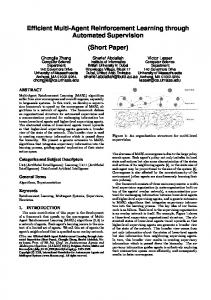
1 Introduction As a joint field of artificial intelligence and modern statistics, machine learning is concerned with the design and development of algorithms and techniques that allow computers to automatically extract information and “learn” structure from data. The learned structure can be described by a statistical model that compactly represents the data. As a branch of machine learning, reinforcement learning (RL) is a computational approach to learning from interactions with the surrounding world and concerned with sequential decision making in unknown environments to achieve high-level goals. Usually, no sophisticated prior knowledge is available and all required information to achieve the goal has to be obtained through trials. The following (pictorial) setup emerged as a general framework to solve this kind of problems (Kaelbling et al., 1996). An agent interacts with its surrounding world by taking actions (see Figure 1.1). In turn, the agent perceives sensory inputs that reveal some information about the state of the world. Moreover, the agent perceives a reward/penalty signal that reveals information about the quality of the chosen action and the state of the world. The history of taken actions and perceived information gathered from interacting with the world forms the agent’s experience. As opposed to supervised and unsupervised learning, the agent’s experience is solely based on former interactions with the world and forms the basis for its next decisions. The agent’s objective in RL is to find a sequence of actions, a strategy, that minimizes an expected long-term cost. Solely describing the world is therefore insufficient to solve the RL problem: The agent must also decide how to use the knowledge about the world in order to make decisions and to choose actions. Since RL is inherently based on collected experience, it provides a general, intuitive, and theoretically powerful framework for autonomous learning and sequential decision making under uncertainty. The general RL concept can be found in solutions to a variety of

world

sensory inputs

action

agent

reward/penalty

Figure 1.1: Typical RL setup: The agent interacts with the world by taking actions. After each action, the agent perceives sensory information about the state of the world and a scalar signal rating the previously chosen action in the previous state of the world.

2

Chapter 1. Introduction

problems including maneuvering helicopters (Abbeel et al., 2007) or cars (Kolter et al., 2010), truckload scheduling (Simao et al., 2009), drug treatment in a medical application (Ernst et al., 2006), or playing games such as Backgammon (Tesauro, 1994). The RL concept is related to optimal control although the fields are traditionally separate: Like in RL, optimal control is concerned with sequential decision making to minimize an expected long-term cost. In the context of control, the world can be identified as the dynamic system, the decision-making algorithm within the agent corresponds to the controller, and actions correspond to control signals. The RL objective can also be mapped to the optimal control objective: Find a strategy that minimizes an expected long-term cost. In optimal control, it is typically assumed that the dynamic system are known. Since the problem of determining the parameters of the dynamic system is typically not dealt with in optimal control, finding a good strategy essentially boils down to an optimization problem. Since the knowledge of the parameterization of the dynamic system is a often requisite for optimal control (Bertsekas, 2005), this parameterization can be used for internal simulations without the need to directly interact with the dynamic system. Unlike optimal control, the general concept of RL does not require expert knowledge, that is, task-specific prior knowledge, or an intricate prior understanding of the underlying world (in control: dynamic system). Instead, RL largely relies upon experience gathered from directly interacting with the surrounding world; a model of the world and the consequences of actions applied to the world are unknown in advance. To gather information about the world, the RL agent has to explore the world. The RL agent has to trade off exploration, which often means to act sub-optimally, and exploitation of its current knowledge to act locally optimally. For illustration purposes, let us consider the maze in Figure 1.2 from the book by Russell and Norvig (2003). The agent denoted by the green disc in the lowerright corner already found a locally optimal path (indicated by the arrows) from previous interactions leading to the high-reward region in the upper-right corner. Although the path avoids the high-cost region, which yields a reward of −20, it is not globally optimal since each step taken by the agent causes a reward of −1. Here, the exploration-exploitation dilemma becomes clearer: Either the agent sticks to the current suboptimal path or it explores new paths, which might be better, but which might also lead to the high-cost region. Potentially even more problematic is that the agent does not know whether there exists a better path than the current one. Due to its fairly general assumptions, RL typically requires many interactions with the surrounding world to find a good strategy. In some cases, however, it can be proven that RL can converge to a globally optimal strategy (Jaakkola et al., 1994). A central issue in RL is to increase the learning efficiency by reducing the number of interactions with the world that are necessary to find a good strategy. One way to increase the learning efficiency is to extract more useful information from collected experience. For example, a model of the world summarizes collected

3

-1

-1

-1 -1

-1

-1

+20

-1

-20

-1

Figure 1.2: The agent (green disc in the lower-right corner) found a suboptimal path to the high-reward region in the upper-right corner. The black square denotes a wall, the numerical values within the squares denote the immediate reward. The arrows represent a suboptimal path to the high-reward region.

experience and can be used for generalization and hypothesizing about the consequences in the world of taking a particular action. Therefore, using a model that represents the world is a promising approach to make RL more efficient. The model of the world is often described by a transition function that maps state-action pairs to successor states. However, when only a few samples from the world are available they can be explained by many transition functions. Let us assume we decide on a single function, say, the most likely function given the collected experience so far. When we use this function to learn a good strategy, we implicitly believe that this most likely function describes the dynamics of the world exactly—everywhere! This is a rather strong assumption since our decision on the most likely function was based on little data. We face the problem that a strategy based on a model that does not describe dynamically relevant regions of the world sufficiently well can have disastrous effects in the world. We would be more confident if we could select multiple “plausible” transition functions, rank them, and learn a strategy based on a weighted average over these plausible models. Gaussian processes (GPs) provide a consistent and principled probabilistic framework for ranking functions according to their plausibility by defining a corresponding probability distribution over functions (Rasmussen and Williams, 2006). When we use a GP distribution on transition functions to describe the dynamics of the world, we can incorporate all plausible functions into the decision-making process by Bayesian averaging according to the GP distribution. This allows us to reason about things we do not know for sure. Thus, GPs provide a practical tool to reduce the problem of model bias, which frequently occurs when deterministic models are used (Atkeson and Schaal, 1997b; Schaal, 1997; Atkeson and Santamar´ıa, 1997). This thesis presents a principled and practical Bayesian framework for efficient RL in continuous-valued domains by imposing fairly general prior assumptions on the world and carefully modeling collected experience. By carefully modeling uncertainties, our proposed method achieves unprecedented speed of learning and an unprecedented degree of automation by reducing model bias in a principled way: Bayesian inference with GPs is used to explicitly incorporate the uncertainty about the world into long-term planning and decision making. Our framework assumes a fully observable world and is applicable to episodic tasks. Hence, our

4

Chapter 1. Introduction

approach combines ideas from optimal control with the generality of reinforcement learning and narrows the gap between control and RL. A logical extension of the proposed RL framework is to consider the case where the world is no longer fully observable, that is, only noisy or partial measurements of the state of the world are available. In such a case, the true state of the world is unknown (hidden/latent), but it can be described by a probability distribution, the belief state. For an extension of our learning framework to this case, we require two ingredients: First, we need to learn the transition function in latent space, a problem that is related to system identification in a control context. Second, if the transition function is known, we need to infer the latent state of the world based on noisy and partial measurements. The latter problem corresponds to filtering and smoothing in stochastic and nonlinear systems. We do not fully address the extension of our RL framework to partially observable Markov decision processes, but we provide first steps in this direction and present an implementation of the forward-backward algorithm for filtering and smoothing targeted at Gaussian-process dynamic systems. The main contributions of this thesis are threefold: • We present pilco (probabilistic inference and learning for control), a practical and general Bayesian framework for efficient RL in continuous-valued state and action spaces when no task-specific expert knowledge is available. We demonstrate the viability of our framework by applying it to learning complicated nonlinear control tasks in simulation and hardware. Across all tasks, we report an unprecedented efficiency in learning and an unprecedented degree of automation. • Due to its generality and efficiency, pilco can be considered a conceptual and practical approach to learning models and controllers when expert knowledge is difficult to obtain or simply not available, which makes system identification hard. • We introduce a robust algorithm for filtering and smoothing in Gaussianprocess dynamic system. Our algorithm belongs to the class of Gaussian filters and smoothers. These algorithms are a requisite for system identification and the extension of our RL framework to partially observable Markov decision processes. Based on well-established ideas from Bayesian statistics and machine learning, this dissertation touches upon problems of approximate Bayesian inference, regression, reinforcement learning, optimal control, system identification, adaptive control, dual control, state estimation, and robust control. We now summarize the contents of the central chapters of this dissertation: Chapter 2: Gaussian Process Regression. We present the necessary background on Gaussian processes, a central tool in this thesis. We focus on motivating the general concepts of GP regression and the mathematical details required for predictions with Gaussian processes when the test input is uncertain.

5 Chapter 3: Probabilistic Models for Efficient Learning in Control. We introduce pilco, a conceptual and practical Bayesian framework for efficient RL. We present experimental results of applying our fully automatic learning framework to challenging nonlinear control problems in computer simulation and hardware. Due to its principled treatment of uncertainties during planning and policy learning, pilco outperforms state-of-the-art RL methods by at least an order of magnitude on the cart-pole swing-up, a common benchmark problem. Additionally, pilco’s learning speed allows for learning control tasks from scratch that have not been successfully learned from scratch before. Chapter 4: Robust Bayesian Filtering and Smoothing in Gaussian-Process Dynamic Systems. We present algorithms for robust filtering and smoothing in Gaussian-process dynamic systems, where both the nonlinear transition function and the nonlinear measurement function are described by GPs. The robustness of both the filter and the smoother profits from exact moment matching during predictions. We provide experimental evidence that our algorithms are more robust than commonly used Gaussian filters/smoothers such as the extended Kalman filter, the cubature Kalman filter, and the unscented Kalman filter.

7

2 Gaussian Process Regression Regression is the problem of estimating a function h given a set of input vectors xi ∈ RD and observations yi = h(xi ) + εi ∈ R of the corresponding function values, where εi is a noise term. Regression problems frequently arise in the context of reinforcement learning, control theory, and control applications. For example, the transitions in a dynamic system are typically described by a stochastic or deterministic function h. Due to finiteness of measurements yi and the presence of noise, the estimate of the function h, is uncertain. The Bayesian framework allows us to express this uncertainty in terms of probability distributions, requiring the concept of distributions over functions—a Gaussian process (GP) provides such a distribution. In a classical control context, the transition function is typically defined by a finite number of parameters φ, which are often motivated by Newton’s laws of motion. These parameters can be considered masses or inertias, for instance. In this context, regression aims to find a parameter set φ∗ such that h(φ∗ , xi ) best explains the corresponding observations yi , i = 1, . . . , n. Within the Bayesian framework, a (posterior) probability distribution over the parameters φ expresses our uncertainty and beliefs about the function h. Often we are interested in making predictions using the model for h. To make predictions at an arbitrary input x∗ , we take the uncertainty about the parameters φ into account by averaging over them with respect to their probability distribution. We then obtain a predictive distribution p(y∗ |x∗ , φ∗ ), which sheds light not only on the expected value of y∗ , but also on the uncertainty of this estimated value. In these so called parametric models, the parameter set φ imposes a fixed structure upon the function h. The number of parameters is determined in advance and independent of the number n of observations, the sample size. Presupposing structure on the function limits its representational power. If the parametric model is too restrictive, we might think that the current set of parameters is not the complete parameter set describing the dynamic system: Often one assumes idealized circumstances, such as massless sticks and frictionless systems. One option to make the model more flexible is to add parameters to φ, which we think they may be of importance. However, this approach quickly gets complicated, and some effects such as slack can be difficult to describe or to identify. At this point, we can go one step back, dispense with the physical interpretability of the system parameters, and employ so called non-parametric models. The basic idea of non-parametric regression is to determine the shape of the underlying function h from the data and higher-level assumptions. The term “nonparametric” does not imply that the model has no parameters, but that the effective number of the parameters is flexible and grows with the sample size. Usually, this means using statistical models that are infinite-dimensional (Wasserman,

8

Chapter 2. Gaussian Process Regression

2006). In the context of non-parametric regression, the “parameters” of interest are the values of the underlying function h itself. High-level assumptions, such as smoothness, are often easier to justify than imposing parametric structure on h. Choosing a flexible parametric model such as a high-degree polynomial or a non-parametric model can lead to overfitting. As described by Bishop (2006), when a model overfits, its expressive power is too high and it starts fitting noise. In this thesis, we will focus on Gaussian process (GP) regression, also known as kriging. GPs are used for state-of-the-art regression and combine the flexibility of non-parametric modeling with tractable Bayesian modeling and inference: Instead of inferring a single function (a point estimate) from data, GPs infer a distribution over functions. In the non-parametric context, this corresponds to dealing with distributions on an infinite-dimensional parameter space (Hjort et al., 2010) when we consider a function being fully specified by an infinitely long vector of function values. Since the GP is a non-parametric model with potentially unbounded complexity, its expressive power is high and underfitting typically does not occur. Additionally, overfitting is avoided by the Bayesian approach to computing the posterior over parameters—in our case, the function itself. We will briefly touch upon this in Section 2.2.3.

2.1

Definition and Model

A Gaussian process is a distribution over functions and a generalization of the Gaussian distribution to an infinite-dimensional function space: Let h1 , . . . , h|T | be a set of random variables, where T is an index set. For |T | < ∞, we can collect these random variables in a random vector h = [h1 , . . . , h|T | ]> . Generally, a vector can be regarded as a function h : i 7→ h(i) = hi with finite domain, i = 1, . . . , |T |, which maps indices to vector entries. For |T | = ∞ the domain of the function is infinite and the mapping is given by h : x 7→ h(x). Roughly speaking, the image of the function is an infinitely long vector. Let us now consider the case (xt )t∈T and h : xt 7→ h(xt ), where h(x1 ), . . . , h(x|T | ) have a joint (Gaussian) distribution. For |T | < ∞ the values h(x1 ), . . . , h(x|T | ) are distributed according to a multivariate Gaussian. For |T | = ∞, the corresponding infinite-dimensional distribution of the random variables h(xt ), t = 1, . . . , ∞ is a stochastic process, more precisely, a Gaussian process. Therefore, a Gaussian distribution and a Gaussian process are different. After this intuitive description, we now formally define the GP as a particular stochastic process: Definition 1 (Stochastic process). A stochastic process is a function b of two arguments {b(t, ω) : t ∈ T, ω ∈ Ω}, where T is an index set, such as time, and Ω is a sample space, such as RD . For fixed t ∈ T , {b(t, ·)} is a collection of random ˚ om, ¨ variables (Astr 2006). Definition 2 (Gaussian process). A Gaussian process is a collection of random variables, any finite number of which have a consistent joint Gaussian distribution ˚ om, ¨ (Astr 2006; Rasmussen and Williams, 2006).

9

2.2. Bayesian Inference

Although the GP framework requires dealing with infinities, all computations required for regression and inference with GPs can be broken down to manipulating multivariate Gaussian distributions as we see later in this chapter. In the standard GP regression model, we assume that the data D := {X := [x1 , . . . , xn ]> , y := [y1 , . . . , yn ]> } have been generated according to yi = h(xi ) + εi , where h : RD → R and εi ∼ N (0, σε2 ) is independent Gaussian measurement noise. GPs consider h a random function and infer a posterior distribution p(h|D) over h from the GP prior p(h), the data D, and high-level assumptions on the smoothness of h. The posterior is used to make predictions about function values h(x∗ ) at arbitrary inputs x∗ ∈ RD . Similar to a Gaussian distribution, which is fully specified by a mean vector and a covariance matrix, a GP is fully specified by a mean function mh ( · ) and a covariance function kh (x, x0 ) := Eh [(h(x) − mh (x))(h(x0 ) − mh (x0 ))] = covh [h(x), h(x0 )] ,

x, x0 ∈ RD , (2.1) which specifies the covariance between any two function values. Here, Eh denotes the expectation with respect to the function h. The covariance function kh ( · , · ) is also called a kernel. Similar to the mean value of a Gaussian distribution, the mean function mh describes how the “average” function is expected to look. The GP definition (see Definition 2) yields that any finite set of function values h(X) := [h(x1 ), . . . , h(xn )] is jointly Gaussian distributed. Using the notion of the mean function and the covariance function, the Gaussian distribution of any finite set of function values h(X) can be explicitly written down as p(h(X)) = N (mh (X), kh (X, X)) ,

(2.2)

where kh (X, X) is the full covariance matrix of all function values h(X) under consideration and N denotes a normalized Gaussian probability density function. The graphical model of a GP is given in Figure 2.1. We denote a function that is GP distributed by h ∼ GP or h ∼ GP(mh , kh ).

2.2

Bayesian Inference

To find a posterior distribution on the (random) function h, we employ Bayesian inference techniques within the GP framework. Gelman et al. (2004) define Bayesian inference as the process of fitting a probability model to a set of data and summarizing the result by a probability distribution on the unknown quantity, in our case the function h itself. Bayesian inference can be considered a three-step procedure: First, a prior on the unknown quantity has to be specified. In our case, the unknown quantity is the function h itself. Second, data are observed. Third, a posterior distribution over h is computed that refines the prior by incorporating evidence from the observations. We go briefly through these steps in the context of GPs.

10


hi

i = x1 , ..., xn Figure 2.1: Factor graph of a GP model. The node hi is a short-hand notation for h(xi ). The plate notation is a compact representation of a n-fold copy of the node hi , i = x1 , . . . , xn . The black square is a factor representing the GP prior connecting all variables hi . In the GP model any finite collection of function values h(x1 ), . . . , h(xn ) has a joint Gaussian distribution.

2.2.1

Prior

When modeling a latent function with Gaussian processes, we place a GP prior p(h) directly on the space of functions. In the GP model, we have to specify the prior mean function and the prior covariance function. Unless stated otherwise, we consider a prior mean function mh ≡ 0 and use the squared exponential (SE) covariance function with automatic relevance determination kSE (xp , xq ) := α2 exp − 12 (xp − xq )> Λ−1 (xp − xq ) , xp , xq ∈ RD , (2.3) plus a noise covariance function δpq σε2 , such that kh = kSE + δpq σε2 . In equation (2.3), Λ = diag([`21 , . . . , `2D ]) is a diagonal matrix of squared characteristic length-scales ì , i = 1, . . . , D, and α2 is the signal variance of the latent function h. In the noise covariance function, δpq denotes the Kronecker symbol that is unity when p = q and zero otherwise, which essentially encodes that the measurement noise is independent.1 With the SE covariance function in equation (2.3) we assume that the latent function h is smooth and stationary. The length-scales `1 , . . . , `D , the signal variance α2 , and the noise variance σε2 are so called hyper-parameters of the latent function, which are collected in the hyper-parameter vector θ. Figure 2.2 is a graphical model that describes the hierarchical structure we consider: The bottom is an observed level given by the data D = {X, y}. Above the data is the latent function h, the random “variable” we are primarily interested in. At the top level, the hyper-parameters θ specify the distribution on the function values h(x). A third level of models Mi , for example different covariance functions, could be added on top. This case is not discussed in this thesis since we always choose a single covariance function. Rasmussen and Williams (2006) provide the details on a three-level inference in the context of model selection. 1 I thank Ed Snelson for pointing out that the Kronecker symbol is defined on the indices of the samples but not on input locations. Therefore, xp and xq are uncorrelated according to the noise covariance function even if xp = xq , but p 6= q.

11


θ

level 2: hyper-parameters

h

level 1: function

D

data

Figure 2.2: Hierarchical model for Bayesian inference with GPs.

Expressiveness of the Model Despite the simplicity of the SE covariance function and the uninformative prior mean function (mh ≡ 0), the corresponding GP is sufficiently expressive in most interesting cases. Inspired by MacKay (1998) and Kern (2000), we motivate this statement by showing the correspondence of our GP model to a universal function approximator: Consider a function N (x − (i + 1 X h(x) = lim γn exp − N →∞ N λ2 n=1 i∈Z X

n 2 )) N

,

x ∈ R,

λ ∈ R+ ,

(2.4)

represented by infinitely many Gaussian-shaped basis functions along the real axis 2 with variance λ2 . Let us also assume a standard-normal prior distribution N (0, 1) on the weights γn , n = 1, . . . , N . The model in equation (2.4) is typically considered a universal function approximator. In the limit N → ∞, we can replace the sums with an integral over R and rewrite equation (2.4) as h(x) =

XZ i∈Z

i

i+1

Z ∞ (x − s)2 (x − s)2 γ(s) exp − ds = γ(s) exp − ds , λ2 λ2 −∞

(2.5)

where γ(s) ∼ N (0, 1). The integral in equation (2.5) can be considered a convolution of the white-noise process γ with a Gaussian-shaped kernel. Therefore, the function values of h are jointly normal and h is a Gaussian process according to Definition 2. Let us now compute the prior mean function and the prior covariance function of h: The only uncertain variables in equation (2.5) are the weights γ(s). Computing the expected function of this model, that is, the prior mean function, requires averaging over γ(s) and yields Z Eγ [h(x)] =

(2.5)

h(x)p(γ(s)) dγ(s) =

Z

Z (x − s)2 exp − γ(s)p(γ(s)) dγ(s) ds = 0 λ2 (2.6)

since Eγ [γ(s)] = 0. Hence, the prior mean function of h equals zero everywhere.

12


Let us now find the prior covariance function. Since the prior mean function equals zero, we obtain Z 0 0 covγ [h(x), h(x )] = Eγ [h(x)h(x )] = h(x)h(x0 )p(γ(s)) dγ(s) (2.7) Z Z (x0 − s)2 (x − s)2 exp − γ(s)2 p(γ(s)) dγ(s) ds , x, x0 ∈ R , = exp − λ2 λ2 (2.8) for the prior covariance function, where we used the definition of h in equation (2.5). With varγ [γ(s)] = 1 and by completing the squares, the prior covariance function is given as ! 2 0 )2 2 0 0 2 Z 2 s − s(x + x0 ) + x +2xx4 +(x ) − xx0 + x +(x 0 2 covγ [h(x), h(x )] = exp − ds λ2 (2.9) Z

exp −

=

2 s−

x+x0 2 2

λ2

+

(x−x0 )2 2

! ds

(x − x0 )2 = α exp − 2λ2 2

(2.10) (2.11)

for suitable α2 . From equations (2.6) and (2.11), we see that the prior mean function and the prior covariance function of the universal function approximator in equation (2.4) correspond to the GP model assumptions we made earlier: a prior mean function mh ≡ 0 and the SE covariance function given in equation (2.3) for a onedimensional input space. Hence, the considered GP prior implicitly assumes latent functions h that can be described by the universal function approximator in equation (2.5). Examples of covariance functions that encode different model assumptions are given in the book by Rasmussen and Williams (2006, Chapter 4). 2.2.2

Posterior

After having observed function values y with yi = h(xi ) + εi , i = 1, . . . , n, for a set of input vectors X, Bayes’ theorem yields p(h|X, y, θ) =

p(y|h, X, θ)p(h|θ) , p(y|X, θ)

(2.12)

the posterior (GP) distribution over h. Note that p(y|h, X, θ) is a finite probability distribution, but the GP prior p(h|θ) is a distribution over functions, an infinitedimensional object. Hence, the (GP) posterior is also infinite dimensional. We assume that the observations yi are conditionally independent given X. Therefore, the likelihood of h factors according to p(y|h, X, θ) =

n Y i=1

p(yi |h(xi ), θ) =

n Y i=1

N (yi | h(xi ), σε2 ) = N (y | h(X), σε2 I) .

(2.13)

13

3

3

2

2

1

1 h(x)

h(x)


0

0

−1

−1

−2

−2

−3 −5

−4

−3

−2

−1

0 x

1

2

3

4

5

(a) Samples from the GP prior. Without any observations, the prior uncertainty about the underlying function is constant everywhere.

−3 −5

−4

−3

−2

−1

0 x

1

2

3

4

5

(b) Samples from the GP posterior after having observed 8 function values (black crosses). The posterior uncertainty varies and depends on the location of the training inputs.

Figure 2.3: Samples from the GP prior and the GP posterior for fixed hyper-parameters. The solid black lines represent the mean functions, the shaded areas represent the 95% confidence intervals of the (marginal) GP distribution. The colored dashed lines represent three sample functions from the GP prior and the GP posterior, Panel (a) and Panel (b), respectively. The black crosses in Panel (b) represent the training targets.

The likelihood in equation (2.13) essentially encodes the assumed noise model. Here, we assume additive independent and identically distributed (i.i.d.) Gaussian noise. For given hyper-parameters θ, the Gaussian likelihood p(y|X, h, θ) in equation (2.13) and the GP prior p(h|θ) lead to the GP posterior in equation (2.12). The mean function and a covariance function of this posterior GP are given by Eh [h(˜ x)|X, y, θ] = kh (˜ x, X)(kh (X, X) + σε2 I)−1 y , (2.14) 0 0 2 −1 0 covh [h(˜ x), h(x )|X, y, θ] = kh (˜ x, x ) − kh (˜ x, X)(kh (X, X) + σε I) kh (X, x ) , (2.15) ˜ , x0 ∈ RD are arbitrary vectors, which we call the test inputs. respectively, where x For notational convenience, we write kh (X, x0 ) for [kh (x1 , x0 ), . . . , kh (xn , x0 )] ∈ Rn×1 . Note that kh (x0 , X) = kh (X, x0 )> . Figure 2.3 shows samples from the GP prior and the GP posterior. With only a few observations, the prior uncertainty about the function has been noticeably reduced. At test inputs that are relatively far away from the training inputs, the GP posterior falls back to the GP prior. This can be seen at the left border of Panel 2.3(b)

2.2.3

Training: Learning Hyper-parameters via Evidence Maximization

Let us have a closer look at the two-level inference scheme in Figure 2.2. Thus far, we determined the GP posterior for a given set of hyper-parameters θ. In the following, we treat the hyper-parameters θ as latent variables since their values are not known a priori. In a fully Bayesian setup, we place a hyper-prior p(θ) on the

14


hyper-parameters and integrate them out, such that Z p(h) = p(h|θ)p(θ) dθ , ZZ p(y|X) = p(y|X, h, θ)p(h|θ)p(θ) dh dθ Z = p(y|X, θ)p(θ) dθ .

(2.16) (2.17) (2.18)

The integration required for p(y|X) is analytically intractable since p(y|X, θ) with log p(y|X, θ) = − 21 y> (Kθ + σε2 I)−1 y − 21 log |Kθ + σε2 I| −

D 2

log(2π)

(2.19)

is a nasty function of θ, where D is the dimension of the input space and K is the kernel matrix with Kij = k(xi , xj ). We made the dependency of K on the hyper-parameters θ explicit by writing Kθ . Approximate averaging over the hyperparameters can be done using computationally demanding Monte Carlo methods. In this thesis, we do not follow the Bayesian path to the end. Instead, we find a ˆ of hyper-parameters on which we condition our inference. good point estimate θ To do so, let us go through the hierarchical inference structure in Figure 2.2. Level-1 Inference When we condition on the hyper-parameters, the GP posterior on the function is p(h|X, y, θ) =

p(y|X, h, θ) p(h|θ) , p(y|X, θ)

(2.20)

where p(y|X, h, θ) is the likelihood of the function h, see equation (2.13), and p(h|θ) is the GP prior on h. The posterior mean and covariance functions are given in equations (2.14) and (2.15), respectively. The normalizing constant Z p(y|X, θ) = p(y|X, h, θ) p(h|θ) dh (2.21) in equation (2.20) is the marginal likelihood, also called the evidence. The marginal likelihood is the likelihood of the hyper-parameters given the data after having marginalized out the function h. Level-2 Inference The posterior on the hyper-parameters is p(θ|X, y) =

p(y|X, θ) p(θ) , p(y|X)

(2.22)

where p(θ) is the hyper-prior. The marginal likelihood at the second level is Z p(y|X) = p(y|X, θ) p(θ) dθ , (2.23) where we average over the hyper-parameters. This integral is analytically inˆ of tractable in most interesting cases. However, we can find a point estimate θ the hyper-parameters. In the following, we discuss how to find this point estimate.

15

2.2. Bayesian Inference Evidence Maximization

When we choose the hyper-prior p(θ), a priori we must not exclude any possible settings of the hyper-parameters. By choosing a “flat” prior, we assume that any values for the hyper-parameters are possible a priori. The flat prior on the hyper-parameters has computational advantages: It makes the posterior distribution over θ (see equation (2.22)) proportional to the marginal likelihood in equation (2.21), that is, p(θ|X, y) ∝ p(y|X, θ). This means the maximum a posteriori (MAP) estimate of the hyper-parameters θ equals the maximum (marginal) likelihood estimate. To find a vector of “good” hyper-parameters, we therefore maximize the marginal likelihood in equation (2.21) with respect to the hyperparameters as recommended by MacKay (1999). In particular, the log-marginal likelihood (log-evidence) is Z log p(y|X, θ) = log p(y|h, X, θ) p(h|θ) dh = − 21 y> (Kθ + σε2 I)−1 y − 21 log |Kθ + σε2 I| − D2 log(2π) . | {z } | {z } data-fit term

(2.24)

complexity term

The hyper-parameter vector ˆ ∈ arg max log p(y|X, θ) θ θ

(2.25)

is called a type II maximum likelihood estimate (ML-II) of the hyper-parameters, which can be used at the bottom level of the hierarchical inference scheme to determine the posterior distribution over h (Rasmussen and Williams, 2006).2 This means, ˆ instead of θ in equations (2.14) and (2.15) for the posterior mean and we use θ covariance functions. For notational convenience, we no longer condition on the ˆ hyper-parameter estimate θ. Evidence maximization yields a posterior GP model that trades off data-fit and model complexity as indicated in equation (2.24. Hence, it avoids overfitting by implementing Occam’s razor, which tells us to use the simplest model that explains the data. MacKay (2003) and Rasmussen and Ghahramani (2001) show that coherent Bayesian inference automatically embodies Occam’s razor. Maximizing the evidence using equation (2.24) is a nonlinear, non-convex optimization problem. This can be hard depending on the data set. However, after optimizing the hyper-parameters, the GP model can always explain the data although a global optimum has not necessarily been found. Alternatives to MLII, such as cross validation or hyper-parameter marginalization, can be employed. Cross validation is computationally expensive; jointly marginalizing out the hyperparameters and the function is typically analytically intractable and requires Monte Carlo methods. ˆ using evidence maximization is called trainThe procedure of determining θ ing. A graphical model of a full GP including training and test sets is given in Figure 2.4. Here, we distinguish between three sets of inputs: training, testing, 2 We computed the ML-II estimate θ ˆ using the gpml-software, which is publicly available at http://www. gaussianprocess.org.

16


hi

hj

hk

yi

yj

yk

i = x1 , ..., xn

j = x∗1 , ..., x∗m

k = xo1 , ..., xoK

training

test

other

Figure 2.4: Factor graph for GP regression. The shaded nodes are observed variables. The factors inside the plates correspond to p(y{i,j,k} |h{i,j,k} ). In the left plate, the variables (xi , yi ), i = 1, . . . , n, denote the training set. The variables x∗j in the center plate are a finite number of test inputs. The corresponding test targets are unobserved. The right-hand plate subsumes any “other” finite set of function values and (unobserved) observations. In GP regression, these “other” nodes are integrated out.

and “other”. Training inputs are the vectors based on which the hyper-parameters have been learned, test inputs are query points for predictions. All “other” variables are marginalized out during training and testing and added to the figure for completeness.

2.3

Predictions

The main focus of this thesis lies on how we can use GP models for reinforcement learning and smoothing. Both tasks require iterative predictions with GPs when the input is given by a probability distribution. In the following, we provide the central theoretical foundations of this thesis by discussing predictions with GPs in detail. We cover both predictions at deterministic and random inputs, and for univariate and multivariate targets. In the following, we always assume a GP posterior, that is, we gathered training data and learned the hyper-parameters using marginal-likelihood maximization. The posterior GP can be used to compute the posterior predictive distribution of h(x∗ ) for any test input x∗ . From now on, we call the “posterior predictive distribution” simply a “predictive distribution” and omit the explicit dependence ˆ of the hyper-parameters. Since we assume that the GP on the ML-II estimate θ has been trained before, we sometimes additionally omit the explicit dependence of the predictions on the training set X, y.

17

2.3. Predictions 2.3.1

Predictions at Deterministic Inputs

From the definition of the GP, the function values for test inputs and training inputs are jointly Gaussian, that is,     mh (X) K kh (X, X∗ ) ,  , p(h, h∗ |X, X∗ ) = N  (2.26) mh (X∗ ) kh (X∗ , X) K∗ where we define h := [h(x1 ), . . . , h(xn )]> and h∗ := [h(x∗1 ), . . . , h(x∗m )]> . “other” function values have been integrated out.

All

Univariate Predictions: x∗ ∈ RD , y∗ ∈ R Let us start scalar training targets yi ∈ R and a deterministic test input x∗ . From equation (2.26), it follows that the predictive marginal distribution p(h(x∗ )|D, x∗ ) of the function value h(x∗ ) is Gaussian. Its mean and variance are given by µ∗ := mh (x∗ ) := Eh [h(x∗ )|X, y] = kh (x∗ , X)(K + σε2 I)−1 y n X = kh (x∗ , X)β = βi kh (xi , x∗ ) ,

(2.27) (2.28)

i=1

σ∗2 := σh2 (x∗ ) := varh [h(x∗ )|X, y] = kh (x∗ , x∗ ) − kh (x∗ , X)(K + σε2 I)−1 kh (X, x∗ ) , (2.29) respectively, where β := (K + σε2 I)−1 y. The predictive mean in equation (2.28) can ¨ therefore be expressed as a finite kernel expansion with weights βi (Scholkopf and Smola, 2002; Rasmussen and Williams, 2006). Note that kh (x∗ , x∗ ) in equation (2.29) is the prior model uncertainty plus measurement noise. From this prior uncertainty, we subtract a quadratic form that encodes how much information we can transfer from the training set to the test set. Since kh (x∗ , X)(K + σε2 I)−1 kh (X, x∗ ) is positive definite, the posterior variance σh2 (x∗ ) is not larger than the prior variance given by kh (x∗ , x∗ ). Multivariate Predictions: x∗ ∈ RD , y∗ ∈ RE If y ∈ RE is a multivariate target, we train E independent GP models using the same training inputs X = [x1 , . . . , xn ], xi ∈ RD , but different training targets ya = [y1a , . . . , yna ]> , a = 1, . . . , E. Under this model, we assume that the function values h1 (x), . . . , hE (x) are conditionally independent given an input x. Within the same dimension, however, the function values are still fully jointly Gaussian. The graphical model in Figure 2.5 shows the independence structure in the model across dimensions. Intuitively, the target values of different dimensions can only “communicate” via x. If x is deterministic, it d-separates the training targets as detailed in the books by Bishop (2006) and Pearl (1988). Therefore, the target values covary only if x is uncertain and we integrate it out. For a known x∗ , the distribution of a predicted function value for a single target dimension is given by the equations (2.28) and (2.29), respectively. Under

18


x hE

h1 h2

h1 (x)

h2 (x)

hE (x)

Figure 2.5: Directed graphical model if the latent function h maps into RE . The function values across dimensions are conditionally independent given the input.

1

h(x)

0.5 0 −0.5

1.5 1 p(h(x))

0.5

0

−1 −1

p(x)

2

−0.5

0 x

0.5

1

−0.5

0

0.5

1

1 0 −1

Figure 2.6: GP prediction at an uncertain test input. To determine the expected function value, we average over both the input distribution (blue, lower-right panel) and the function distribution (GP model, upper-right panel). The exact predictive distribution (shaded area, left panel) is approximated by a Gaussian (blue, left panel) that possesses the mean and the covariance of the exact predictive distribution (moment matching). Therefore, the blue Gaussian distribution q in the left panel is the optimal Gaussian approximation of the true distribution p since it minimizes the Kullback-Leibler divergence KL(p||q).

the model described by Figure 2.5, the predictive distribution of h(x∗ ) is Gaussian with mean and covariance h i> (2.30) µ∗ = mh1 (x∗ ) . . . mhE (x∗ ) , h i Σ∗ = diag σh21 . . . σh2E , (2.31) respectively. 2.3.2

Predictions at Uncertain Inputs

In the following, we discuss how to predict with Gaussian processes when the test input x∗ has a probability distribution. Many derivations in the following are based ˜ on the thesis by Kuss (2006) and the work by Quinonero-Candela et al. (2003a,b). Consider the problem of predicting a function value h(x∗ ), h : RD → R, at an uncertain test input x∗ ∼ N (µ, Σ), where h ∼ GP with an SE covariance function kh plus a noise covariance function. This situation is illustrated in Figure 2.6. The input distribution p(x∗ ) is the blue Gaussian in the lower-right panel. The upper-right panel shows the posterior GP represented by the posterior mean function (black) and twice the (marginal) standard deviation (shaded). Generally, if a

2.3. Predictions

19

Gaussian input x∗ ∼ N (µ, Σ) is mapped through a nonlinear function, the exact predictive distribution Z p(h(x∗ )|µ, Σ) = p(h(x∗ )|x∗ )p(x∗ |µ, Σ) dx∗ (2.32) is not Gaussian and unimodal as shown in the left panel of Figure 2.6, where the shaded area represents the exact distribution over function values. On the left-hand-side in equation (2.32), we conditioned on µ and Σ to indicate that the test input x∗ is uncertain. As mentioned before, we omitted the conditioning on the ˆ By explicitly conditioning training data X, y and the posterior hyper-parameters θ. on x∗ in p(h(x∗ )|x∗ ), we emphasize that x∗ is a deterministic argument of h in this conditional distribution. Generally, the predictive distribution in equation (2.32) cannot be computed analytically since a Gaussian distributions mapped through a nonlinear function (or GP) leads to a non-Gaussian predictive distribution. In the considered case, however, we approximate the predictive distribution p(h(x∗ )|µ, Σ) by a Gaussian (blue in left panel of Figure 2.6) that possesses the same mean and variance (moment matching). To determine the moments of the predictive function value, we average over both the input distribution and the distribution of the function given by the GP. Univariate Predictions: x∗ ∼ N (µ, Σ) ∈ RD , y∗ ∈ R Suppose x∗ ∼ N (µ, Σ) is a Gaussian distributed test point. The mean and the variance of the GP predictive distribution for p(h(x∗ )|x∗ ) in the integrand in equation (2.32) are given in equations (2.28) and (2.29), respectively. For the SE kernel, we can compute the mean µ∗ and the variance σ∗2 of the predictive distribution in equation (2.32) in closed form.3 The mean µ∗ can be computed using the law of iterated expectations (Fubini’s theorem) and is given by ZZ µ∗ = h(x∗ )p(h, x∗ ) d(h, x∗ ) = Ex∗ ,h [h(x∗ )|µ, Σ] = Ex∗ [Eh [h(x∗ )|x∗ ]|µ, Σ] (2.33) Z (2.28) (2.28) (2.34) = Ex∗ [mh (x∗ )|µ, Σ] = mh (x∗ )N (x∗ | µ, Σ) dx∗ = β > q , where q = [q1 , . . . , qn ]> ∈ Rn with Z qi := kh (xi , x∗ )N (x∗ | µ, Σ) dx∗ 1 = α2 |ΣΛ−1 + I|− 2 exp − 12 (xi − µ)> (Σ + Λ)−1 (xi − µ) .

(2.35) (2.36)

Each qi is an expectation of kh (xi , x∗ ) with respect to the probability distribution of x∗ . This means that qi is the expected covariance between the function values h(xi ) and h(x∗ ). Note that the predictive mean in equation (2.34) depends explicitly 3 This statement holds for all kernels, for which the integral of the kernel times a Gaussian can be computed analytically. In particular, this is true for kernels that involve polynomials, squared exponentials, and trigonometric functions.

20


on the mean and covariance of the distribution of the input x∗ . The values qi in equation (2.36) correspond to the standard SE kernel kh (xi , µ), which has been “inflated” by Σ. For a deterministic input x∗ with Σ ≡ 0, we obtain µ = x∗ and recover qi = kh (xi , x∗ ). Then, the predictive mean (2.34) equals the predictive mean for certain inputs given in equation (2.28). Using Fubini’s theorem, we obtain the variance σ∗2 of the predictive distribution p(h(x∗ )|µ, Σ) as σ∗2 = varx∗ ,h [h(x∗ )|µ, Σ] = Ex∗ [varh [h(x∗ )|x∗ ]|µ, Σ] + varx∗ [Eh [h(x∗ )|x∗ ]|µ, Σ] (2.37) (2.38) = Ex∗ [σh2 (x∗ )|µ, Σ] + Ex∗ [mh (x∗ )2 |µ, Σ] − Ex∗ [mh (x∗ )|µ, Σ]2 , where we used mh (x∗ ) = Eh [h(x∗ )|x∗ ] and σh2 (x∗ ) = varh [h(x∗ )|x∗ ], respectively. By taking the expectation with respect to the test input x∗ and by using equation (2.28) for mh (x∗ ) and equation (2.29) for σh2 (x∗ ) we obtain σ∗2

Z

=

kh (x∗ , x∗ ) − kh (x∗ , X)(K + σε2 I)−1 kh (X, x∗ )p(x∗ ) dx∗ Z + kh (x∗ , X) ββ > kh (X, x∗ ) p(x∗ ) dx∗ − (β > q)2 , | {z } | {z } 1×n

(2.39)

n×1

where we additionally used Ex∗ [mh (x∗ )|µ, Σ] = β > q from equation (2.34). Plugging in the definition of the SE kernel in equation (2.3) for kh , the desired predicted variance at an uncertain input x∗ is σ∗2

2

σε2 I)−1

Z

= α − tr (K + kh (X, x∗ )kh (x∗ , X)p(x∗ ) dx∗ Z > +β kh (X, x∗ )kh (x∗ , X)p(x∗ ) dx∗ β − (β > q)2 | {z }

(2.40)

˜ =:Q

˜ + = α2 − tr (K + σε2 I)−1 Q | {z } =Ex∗ [varh [h(x∗ )|x∗ ]|µ,Σ]

˜ − µ2 β > Qβ {z }∗ |

,

(2.41)

=varx∗ [Eh [h(x∗ )|x∗ ]|µ,Σ]

where we re-arranged the inner products to pull the expressions that are indepen˜ ∈ Rn×n are given by dent of x∗ out of the integrals. The entries of Q ˜ ij = kh (xi , µ)kh (xj ,1µ) exp (˜zij − µ)> (Σ + 1 Λ)−1 ΣΛ−1 (˜zij − µ) Q 2 |2ΣΛ−1 + I| 2

(2.42)

with z˜ij := 21 (xi + xj ). Like the predicted mean in equation (2.34), the predictive variance depends explicitly on the mean µ and the covariance matrix Σ of the input distribution p(x∗ ).

21

2.3. Predictions Multivariate Predictions: x∗ ∼ N (µ, Σ) ∈ RD , y∗ ∈ RE

In the multivariate case, the predictive mean vector µ∗ of p(h(x∗ )|µ, Σ) is the collection of all E independently predicted means computed according to equation (2.34). We obtain the predicted mean i> h > , µ∗ |µ, Σ = β > 1 q1 . . . β E q E

(2.43)

where the vectors qi for all target dimensions i = 1, . . . , E are given by equation (2.36). Unlike predicting at deterministic inputs, the target dimensions now covary (see Figure 2.5), and the corresponding predictive covariance matrix   varh,x∗ [h∗1 |µ, Σ] . . . covh,x∗ [h∗1 , h∗E |µ, Σ]     .. .. .. Σ∗ |µ, Σ =  (2.44) .  . .   covh,x∗ [h∗E , h∗1 |µ, Σ] . . . varh,x∗ [h∗E |µ, Σ] is no longer diagonal. Here, ha (x∗ ) is abbreviated by h∗a , a ∈ {1, . . . , E}. The variances on the diagonal are the predictive variances of the individual target dimensions given in equation (2.41). The cross-covariances are given by covh,x∗ [h∗a , h∗b |µ, Σ] = Eh,x∗ [h∗a h∗b |µ, Σ] − µ∗a µ∗b .

(2.45)

With p(x∗ ) = N (x∗ | µ, Σ) we obtain (2.34) Eh,x∗ [h∗a h∗b |µ, Σ] =

(2.28) Ex∗ Eha [h∗a |x∗ ] Ehb [h∗b |x∗ ]|µ, Σ =

Z

mah (x∗ )mbh (x∗ )p(x∗ ) dx∗ (2.46)

due to the conditional independence of ha and hb given x∗ . According to equation (2.28), the mean function mah is mah (x∗ ) = kha (x∗ , X) (Ka + σε2a I)−1 ya , {z } |

(2.47)

=:β a

which leads to Eh,x∗ [h∗a

(2.46) h∗b |µ, Σ] =

Z

(2.47)

Z

mah (x∗ )mbh (x∗ )p(x∗ ) dx∗

(2.48)

k a (x∗ , X)β a khb (x∗ , X)β b p(x∗ ) dx∗ }| {z } | h {z

(2.49)

kha (x∗ , X)> khb (x∗ , X)p(x∗ ) dx∗ β b , | {z }

(2.50)

=

= β> a

Z

∈R

∈R

=:Q

22


where we re-arranged the inner products to pull terms out of the integral that are independent of the test input x∗ . The entries of Q are given by 1

−1 −2 Qij = αa2 αb2 |(Λ−1 a + Λb )Σ + I|

× exp − 21 (xi − xj )> (Λa + Λb )−1 (xi − xj )

−1 −1 × exp − 21 (ˆzij − µ)> ((Λ−1 + Σ)−1 (ˆzij − µ) , a + Λb ) zîj := Λb (Λa + Λb )−1 xi + Λa (Λa + Λb )−1 xj .

(2.51) (2.52)

−1 −1 −1 We define R := Σ(Λ−1 a +Λb )+I, ζ i := (xi −µ), and zij := Λa ζ i +Λb ζ j . Using the matrix inversion lemma from Appendix A.4, we obtain an equivalent expression

Qij =

ka (xi , µ)kb (xj , µ) p exp |R|

n2ij = 2(log(αa )+log(αb ))

1 > −1 z R Σzij 2 ij

exp(n2ij ) , = p |R|

> −1 > −1 −1 ζ> i Λa ζ i + ζ j Λb ζ j − zij R Σzij − , 2

(2.53) (2.54)

where we wrote ka = exp(log(ka )) and kb = exp(log(kb )) for a numerically relatively stable implementation: • Due to limited machine precision, the multiplication of exponentials in equation (2.51) is reformulated as an exponential of a sum. • No matrix inverse of potentially low-rank matrices, such as Σ, is required. In particular, the formulation in equation (2.53) allows for a (fairly inefficient) computation of the predictive covariance matrix if the test input is deterministic, that is, Σ ≡ 0.

−1 −1 We emphasize that R−1 Σ = (Λa−1 + Λ−1 is symmetric. The matrix Q b + Σ ) depends on the covariance of the input distribution as well as on the SE kernels ˜ in equation (2.42) for identical kha and khb . Note that Q in equation (2.53) equals Q target dimensions a = b. To summarize, the entries of the covariance matrix of the predictive distribution are   ∗ ∗  β> a 6= b a Qβ b − Eh,x∗ [ha |µ, Σ] Eh,x∗ [hb |µ, Σ] , ∗ ∗ cov[ha , hb |µ, Σ] =   β > Qβ − Eh,x [h∗ |µ, Σ]2 + α2 − tr (Ka + σ 2 I)−1 Q , a = b . ∗ a a a a ε

(2.55)

If a = b, we have to include the term Ex∗ [covh [ha (x∗ ), hb (x∗ )|x∗ ]|µ, Σ] = αa2 −tr (Ka + σε2 I)−1 Q , which equals zero for a 6= b due to the assumption that the target dimensions a and b are conditionally independent given the input as depicted in the graphical model in Figure 2.5. The function implementing multivariate predictions at uncertain inputs is given in Appendix E.1. These results yield the exact mean µ∗ and the exact covariance Σ∗ of the generally non-Gaussian predictive distribution p(h(x∗ )|µ, Σ), where h ∼ GP and x∗ ∼ N (µ, Σ). Table 2.1 summarizes how to predict with Gaussian processes.

23

2.3. Predictions Table 2.1: Predictions with Gaussian processes—overview.

predictive mean

deterministic test input x∗

random test input x∗ ∼ N (µ, Σ)

univariate

eq. (2.28)

eq. (2.34)

multivariate

eq. (2.30)

eq. (2.43)

univariate

eq. (2.29)

eq. (2.41)

multivariate

eq. (2.31)

eq. (2.44), eq. (2.55)

predictive covariance

2.3.3

Input-Output Covariance

It is sometimes necessary to compute the covariance Σx∗ ,h between a test input x∗ ∼ N (µ, Σ) and the corresponding predicted function value h(x∗ ) ∼ N (µ∗ , Σ∗ ). As an example suppose that the joint distribution     µ Σ Σx∗ ,h∗  (2.56) p(x∗ , h(x∗ )|µ, Σ) = N   ,  > Σ∗ µ∗ Σx∗ ,h∗ is desired. The marginal distributions of x∗ and h(x∗ ) are either given or computed according to Section 2.3.2. The missing piece is the cross-covariance matrix Σx∗ ,h∗ = Ex∗ ,h [x∗ h(x∗ )> ] − Ex∗ [x∗ ] Ex∗ ,h [h(x∗ )]> = Ex∗ ,h [x∗ h(x∗ )> ] − µµ> ∗ ,

(2.57)

which will be computed in the following. For each target dimension a = 1, . . . , E, we compute Ex∗ ,ha [x∗ ha (x∗ )|µ, Σ] as Z Ex∗ ,ha [x∗ ha (x∗ )|µ, Σ] = Ex∗ [x∗ Eha [ha (x∗ )|x∗ ]|µ, Σ] = x∗ mah (x∗ )p(x∗ ) dx∗ (2.58) ! Z n X (2.28) = x∗ βai kha (x∗ , xi ) p(x∗ ) dx∗ , (2.59) i=1

where we used the representation of mh (x∗ ) by means of a finite kernel expansion. By pulling all constants (in x∗ ) out of the integral and swapping summation and integration, we obtain Z n X Ex∗ ,ha [x∗ ha (x∗ )|µ, Σ] = βai x∗ kha (x∗ , xi )p(x∗ ) dx∗ (2.60) =

i=1 n X i=1

where we defined kha (x∗ , xi )

Z βai

x∗ c1 N (x∗ |xi , Λa ) N (x∗ |µ, Σ) dx∗ , | {z }| {z } a (x ,x ) =kh ∗ i

D

1

− − −2 2 |Λa | 2 , c−1 1 := αa (2π)

(2.61)

p(x∗ )

(2.62)

such that = c1 N (x∗ | xi , Λa ) is a normalized Gaussian probability distribution in the test input x∗ , where xi , i = 1, . . . , n, are the training inputs. The

24


product of the two Gaussians in equation (2.61) results in a new (unnormalized) Gaussian c−1 2 N (x∗ | ψ i , Ψ) with 1 D − − 2 |Λa + Σ| 2 exp − 1 (xi − µ)> (Λa + Σ)−1 (xi − µ) , (2.63) c−1 2 = (2π) 2 −1 −1 −1 (2.64) Ψ = (Λa + Σ ) , −1 −1 (2.65) ψ i = Ψ(Λa xi + Σ µ) . Pulling all constants (in x∗ ) out of the integral in equation (2.61), the integral determines the expected value of the product of the two Gaussians, ψ i . Hence, we obtain n X Ex∗ ,ha [x∗ ha (x∗ )|µ, Σ] = (2.66) c1 c−1 2 βai ψ i , a = 1, . . . , E , covx∗ ,h∗ [x∗ , ha (x∗ )|µ, Σ] =

i=1 n X i=1

c1 c−1 2 βai ψ i − µ(µ∗ )a , a = 1, . . . , E .

(2.67)

We now recognize that c1 c−1 = qai , see equation (2.36), and with ψ i = Σ(Σ + 2 Λa )−1 xi + Λ(Σ + Λa )−1 µ, we can simplify equation (2.67). We move the term µ(µ∗ )a into the sum, use equation (2.34) for (µ∗ )a , and obtain covx∗ ,h∗ [x∗ , ha (x∗ )|µ, Σ] =

n X i=1

βai qai Σ(Σ + Λa )−1 xi + (Λa (Σ + Λa )−1 − I)µ (2.68)

=

n X i=1

βai qai Σ(Σ + Λa )−1 (xi − µ) + (Λa (Σ + Λa )−1 + Σ(Σ + Λa )−1 − I)µ (2.69)

=

n X i=1

βai qai Σ(Σ + Λa )−1 (xi − µ) ,

(2.70)

which fully determines the joint distribution p(x∗ , h(x∗ )|µ, Σ) in equation (2.56). An efficient implementation that computes input-output covariances is given in Appendix E.1. 2.3.4

Computational Complexity

For an n-sized training set, training a GP using gradient-based evidence maximization requires O(n3 ) computations per gradient step due to the inversion of the kernel matrix K in equation (2.24). For E different target dimensions, this sums up to O(En3 ) operations. Predictions at uncertain inputs according to Section 2.3.2 require O(E 2 n2 D) operations: • Computing Q ∈ Rn×n in equation (2.53) is computationally the most demanding operation and requires a D-dimensional scalar product per entry, which gives a computational complexity of O(Dn2 ). Here, D is the dimensionality of the training inputs.

2.4. Sparse Approximations using Inducing Inputs

25

• The matrix Q has to be computed for each entry of the predictive covariance matrix Σ∗ ∈ RE×E , where E is the dimension of the training targets, which gives a total computational complexity of O(E 2 n2 D).

2.4

Sparse Approximations using Inducing Inputs

A common problem in training and predicting with Gaussian processes is that the computational burden becomes prohibitively expensive when the size of the data set becomes large. Sparse GP approximations aim to reduce the computational burden associated with training and predicting. The computations in a full GP are dominated by either the inversion of the n × n kernel matrix K or the multiplication of K with vectors, see equations (2.24), (2.28), (2.29), (2.41), and (2.42) for some examples. Typically, sparse approximations aim to find a low-rank approximation ˜ of K. Quinonero-Candela and Rasmussen (2005) describe several sparse approximations within a unifying framework. In the following, we briefly touch upon one class of sparse approximations. For fixed hyper-parameters, the GP predictive distribution in equations (2.28) and (2.29) can be considered essentially parameterized by the training inputs X and the training targets y. Snelson and Ghahramani (2006), Snelson (2007), and Titsias (2009) introduce sparse GP approximations using inducing inputs. A repre¯ of size M is ¯ h} sentative pseudo-training set of fictitious (pseudo) training data {X, ¯ introduced. The inducing inputs are the pseudo training targets h. With the prior ¯ ∼ N (0, KM M ), equation (2.26) can be written as h|¯X Z ¯ h) ¯ dh ¯, p(h, h∗ ) = p(h, h∗ |h)p( (2.71) ˜ where the inducing inputs are integrated out. Quinonero-Candela and Rasmussen (2005) show that most sparse approximations assume that the test targets h and the ¯ that is, training targets h∗ are conditionally independent given the pseudo inputs h, ¯ ¯ ¯ p(h, h∗ |h) = p(h|h)p(h∗ |h). The posterior distribution over the pseudo targets can be computed analytically and is again Gaussian as shown bySnelson and Ghahramani (2006), Snelson (2007), and Titsias (2009). Therefore, the pseudo targets can always be integrated out analytically—at least in the standard GP regression model. ¯ Like in the standard It remains to determine the pseudo-input locations X. GP regression model, Snelson and Ghahramani (2006), Snelson (2007), and Titsias ¯ by evidence maximization. The GP pre(2009) find the pseudo-input locations X dictive distribution from the pseudo-data set is used as a parameterized marginal likelihood Z ¯ h| ¯ X) ¯ ¯ = p(y|X, X, ¯ h)p( ¯ dh p(y|X, X) (2.72) Z ¯ ¯ ¯ (2.73) = N y | KnM K−1 M M h, Γ N h | 0, KM M dh = N (y | 0, Qnn + Γ) ,

(2.74)

26


¯ have been integrated out and where the pseudo-targets h Qnn := KnM K−1 M M KM n ,

¯ X) ¯ . KM M := kh (X,

(2.75)

Qnn is a low-rank approximation of the full-rank kernel matrix Knn = kh (X, X).4 The matrix Γ ∈ {ΓFITC , ΓVB } depends on the type of the sparse approximation. Snelson and Ghahramani (2006) use ΓFITC := diag(Knn − Qnn ) + σε2 I ,

(2.76)

whereas Titsias (2009) employs the matrix ΓVB := σε2 I ,

(2.77)

which is in common with previous sparse approximations by Silverman (1985), Wahba et al. (1999), Smola and Bartlett (2001), Csato´ and Opper (2002), and Seeger et al. (2003), which are not discussed further in this thesis. Using the Γ-notation, the log-marginal likelihood of the sparse GP methods by Titsias (2009) and Snelson and Ghahramani (2006) and Snelson (2007) is given by ¯ = − 1 log |Qnn + Γ| − 1 y> (Qnn + Γ)−1 y − n log(2π) − 1 2 tr(Knn − Qnn ) , log p(y|X, X) 2 2 2 2σ {z } | ε only used by VB

(2.78) where the last term can be considered a regularizer and is solely used in the variational approximation by Titsias (2009). The methods by Snelson and Ghahramani (2006) and Titsias (2009) therefore use different marginal likelihood functions to be maximized. The parameters to be optimized are the hyper-parameters of the ¯ In particular, Titsias (2009) found a covariance function and the input locations X. principled way of sidestepping possible overfitting issues by maximizing a variational lower bound of the true log marginal likelihood, that is, he attempts to minimize the KL divergence KL(q||p) between the approximate marginal likelihood q in equation (2.78) and the true marginal likelihood p in equation (2.24). With the matrix inversion lemma in Appendix A.4, the matrix operations in equation (2.78) no longer need to invert full n × n matrices. We rewrite −1 (Qnn + Γ)−1 = (KnM K−1 M M KM n + Γ) = Γ−1 − Γ−1 KnM (KM M + KM n Γ−1 KnM )−1 KM n Γ−1 , log |Qnn + Γ| = log |KnM K−1 M M KM n + Γ| −1 = log |Γ||K−1 M M ||KM M + KM n Γ KnM | = log |Γ| − log |KM M | + log |KM M + KM n Γ−1 KnM | ,

(2.79) (2.80) (2.81) (2.82) (2.83)

where the inversion of Γ ∈ Rn×n is computationally cheap since Γ is a diagonal matrix. The predictive distribution at a test input x∗ is given by the mean and the variance ¯ −1 KM n Γ−1 y , Eh [h(x∗ )] = kh (x∗ , X)B −1 −1 ¯ ¯ varh [h(x∗ )] = kh (x∗ , x∗ ) − kh (x∗ , X)(K M M − B )kh (X, x∗ ) , 4 For

clarity, we added the subscripts that describe the dimensions of the corresponding matrices.

(2.84) (2.85)

2.5. Further Reading

27

respectively, with B := KM M + KM n Γ−1 KnM . One key difference between the algorithms is that the algorithm by Snelson (2007) can be interpreted as a GP with heteroscedastic noise (note that ΓFITC in equation (2.76) depends on the data), whereas the variational approximation by Titsias (2009) maintains a GP with homoscedastic noise resembling the original GP model. Note that both sparse methods are not degenerate, that is, they have reasonable variances far away from the data. By contrast, in a radial basis function network or in the relevance vector machine the predictive variances collapse to ˜ zero far away from the means of the basis functions (Rasmussen and QuinoneroCandela, 2005). Recently, a new algorithm for sparse GPs was provided by Walder et al. (2008), who generalize the FITC approximation by Snelson and Ghahramani (2006) to the case where the basis functions centered at the inducing input locations can have different length-scales. However, we have not yet thoroughly investigated their multi-scale sparse GPs. 2.4.1

Computational Complexity

Let M be the size of the pseudo training set, and n be the size of the real data set with M n. The sparse approximations allow for training a GP in O(nDM 2 ) (see equation (2.78)) and predicting in O(DM ) for the mean in equation (2.84) and O(DM 2 ) for the variance in equation (2.85), respectively, where D is the dimension of the input vectors. Note that the vector B−1 KM n Γ−1 y and the matrix K−1 MM − −1 B can be computed in advance since they are independent of x∗ . Multivariate predictions (at uncertain inputs) then require O(M E) computations for the mean vector and O(E 2 M 2 D) computations for the covariance matrix.

2.5

Further Reading

In geostatistics and spatial statistics, Gaussian processes are known as kriging. Classical references for kriging are the books by Matheron (1973), Cressie (1993), and Stein (1999). O’Hagan (1978) first describes GPs as a non-parametric prior over functions. Neal (1996, Chapter 2.1) shows that a neural network converges to a GP if the number of hidden units tends to infinity and the weights and the biases have zero-mean Gaussian priors. Williams (1995), Williams and Rasmussen (1996), MacKay (1998), and Rasmussen (1996) introduced GPs into the machine learning community. For details on Gaussian processes in the context of machine learning, we refer to the books by Rasmussen and Williams (2006), Bishop (2006), and MacKay (2003). GP predictions at uncertain inputs have previously been discussed in the pa˜ pers by Girard et al. (2002, 2003), Quinonero-Candela et al. (2003a,b), Kuss (2006), and Ko et al. (2007a). All methods approximate the true predictive distribution by a Gaussian distribution. Ko et al. (2007a) use either a first-order Taylor series expansion of the mean function or a deterministic sampling method to obtain approximate moments of the true predictive distribution. Girard et al. (2002, 2003)

28


use a second-order Taylor series expansion of the mean function and the covariance ˜ function to compute the predictive moments approximately. Quinonero-Candela et al. (2003a,b) derive the analytic expressions for the exact predictive moments and show its superiority over the second-order Taylor series expansion employed by Girard et al. (2002, 2003). ˜ For an overview of sparse approximations, we refer to the paper by QuinoneroCandela and Rasmussen (2005), which gives a unifying view on most of the sparse approximations presented throughout the last decades, such as those by Silverman (1985), Wahba et al. (1999), Smola and Bartlett (2001), Csato´ and Opper (2002), Seeger et al. (2003), Titsias (2009), Snelson and Ghahramani (2006), Snelson (2007), Walder et al. (2008), or Lázaro-Gredilla et al. (2010).

29

3 Probabilistic Models for Efficient Learning in Control Automatic control of dynamic systems has been a major discipline in engineering for decades. Generally, by using a controller, external signals can be applied to a dynamic system to modify its state. The state fully describes the system at a particular point in time. Example 1. Consider an autopilot in an aircraft: Based on sensor measurements the autopilot guides the aircraft without assistance from a human being. The autopilot controls the thrust, the flap angles, and the rudder of the airplane during the flight (level), but also during takeoff and landing. In the aircraft example, the autopilot is called the controller, the entity of the aircraft is the system, and thrust, flap angles, and the rudder are to be controlled. Typically, the controller is designed by a skilled engineer, the expert, to drive the system in an optimal way. Often, the first step toward controller design is a (graybox) system identification by the expert. Roughly speaking, the expert proposes a parametric model structure of the underlying system and identifies its parameters using measured data from the system. Example 2 (Mass-spring system). Let us consider the mass-spring mechanical system described in Figure 3.1. The mathematical formulation of the system’s dynamFsp

F mass spring

Figure 3.1: Simplified mass-spring system described in the book by Khalil (2002). The mass is subjected to an external force F . The restoring force of the spring is denoted by Fsp .

ics is given by Newton’s law of motion. Example parameters to be identified are the mass of the block or the spring constant. One issue with the classical approach to automatic control is that it often relies on idealized assumptions1 and expert knowledge to derive the mathematical formulation for each system. The expert is assumed to have an intricate understanding of the properties of system’s dynamics and the control task. Depending 1 Often, the parameters of a dynamic system are assumed to follow Newton’s laws of motion exactly, which we call “idealized” assumptions.

30

Chapter 3. Probabilistic Models for Efficient Learning in Control

on the nature of the system, expert knowledge might not be available or may be expensive to obtain. Sometimes, neither valid idealized assumptions about a dynamic system can be made due to the complexity of the dynamics or too many hidden parameters nor sufficient expert knowledge is available. Then, (computational) learning techniques can be a valuable complement to automatic control. Because of this, learning algorithms have been used more often in automatic control and robotics during the last decades. In particular, in the context of system identification, learning has been employed to reduce the dependency on idealized assumptions, see, for example, the papers by Atkeson et al. (1997a,b), Vijayakumar and Schaal (2000), Kocijan et al. (2003), Murray-Smith et al. (2003), Grancharova et al. (2008), or Kober and Peters (2009). A learning algorithm can be considered a method to automatically extract relevant structure from data. The extracted information can be used to learn a model of the system dynamics. Subsequently, the model can be used for predictions and decision making by speculating about the long-term consequences of particular actions. Computational approaches for artificial learning from collected data, the experience, are studied in neuroscience, reinforcement learning (RL), approximate dynamic programming, and adaptive control, amongst others. Although these fields have been studied for decades, the rate at which artificial systems learn lags typically behind biological learners with respect to the amount of experience, that is, the data used for learning, required to learn a task if no expert knowledge is available. Experience can be gathered by direct interaction with the environment. Interaction, however, can be time consuming or wear out mechanical systems. Hence, a central issue in RL is to speed up artificial learning algorithms by making them more efficient in terms of required interactions with the system. Broadly, there are two ways to increase the (interaction) efficiency of RL. One approach is to exploit expert knowledge to constrain the task in various ways and to simplify learning. This approach is problem dependent and relies on an intricate understanding of the characteristics of the task and the solution. A second approach to making RL more efficient is to extract more useful information from available experience. This approach does not rely on expert knowledge, but requires careful modeling of available data. In a practical application, one would typically combine these two approaches. In this thesis, however, we are solely concerned with the second approach:

How can we learn as fast as possible given only very general prior understanding of a task?

Thus, we do not look for an engineering solution to a particular problem. Instead, we elicit a general and principled framework for efficiently learning dynamics and controllers.

31 To achieve our objective, we exploit two properties that make biological experience-based learning so efficient: First, humans can generalize from current experience to unknown situations. Second, humans explicitly model and incorpo¨ rate uncertainty when making decisions as, experimentally shown by Kording and Wolpert (2004a, 2006). Unlike for discrete domains (Poupart et al., 2006), generalization and incorporation of uncertainty into planning and the decision-making process are not consistently and fully present in continuous RL, although impressively successful heuristics exist (Abbeel et al., 2006). In the context of motor control, generalization typically requires a model or a simulator, that is, an internal representation of the (system) dynamics. Learning models of the system dynamics is well studied in the literature, see for example the work by Sutton (1990), Atkeson et al. (1997a), or Schaal (1997). These learning approaches for parametric or non-parametric system identification rely on the availability of sufficiently many data to learn an “accurate” system model. As already pointed out by Atkeson and Schaal (1997a) and Atkeson and Santamar´ıa (1997), an “inaccurate” model used for planning often leads to a useless policy in the real world. Now we have the following dilemma: On the one hand we want to speed up RL (reduce the number of interactions with the physical system to learn tasks) by using models for internal simulations, on the other hand existing model-based RL methods still require many interactions with the system to find a sufficiently accurate dynamics model. In this thesis, we bridge this gap by carefully modeling and representing uncertainties about the dynamics model, which allows us to deal with fairly limited experience in a principled way: • Instead of following the standard approach of fitting a deterministic function to the data using neural networks or radial basis function networks, for example, we explicitly require a probabilistic dynamics model. With a probabilistic model, we are able to represent and quantify uncertainty about the learned model. This allows for a coherent generalization of available experience to unknown situations. • The model uncertainty must be incorporated into the decision-making process by averaging over it. Without this probabilistic model-based treatment, the learning algorithm can heavily suffer from model bias as mentioned by Atkeson and Santamar´ıa (1997) and Schaal (1997) and/or can require many interactions with the dynamic system. With pilco (probabilistic inference and learning for control), we present a general and fully Bayesian framework for efficient autonomous learning, planning, and decision making in a control context. Pilco’s success is due to a principled use of probabilistic dynamics models and embodies our requirements of a faithful representation and careful incorporation of available experience into decision making. Due to its principled treatment of uncertainties, pilco does not rely on task-specific expert knowledge, but still allows for efficient learning from scratch. To the best of our knowledge, pilco is the first continuous RL algorithm that consistently

32


ut−1

ut

ut+1

xt−1

xt

xt+1

ct−1

ct

ct+1

Figure 3.2: Directed graphical model for the problem setup. The state x of the dynamic system follows Markovian dynamics and can be influenced by applying external controls u. The cost ct := c(xt ) is either computed or can be observed.

combines generalization and incorporation of uncertainty into planning and the decision-making.

3.1

Setup and Problem Formulation

We consider discrete-time control problems with continuous-valued states x ∈ RD and external control signals (actions) u ∈ RF . The dynamics of the system are described by a Markov decision process (MDP), a computational framework for decision-making under uncertainty. An MDP is a tuple of four objects: the state space, the control space (also called the action space), the one-step transition function f , and an immediate cost function c(x) that evaluates the quality of being in state x. If not stated otherwise, we assume that all states can be measured exactly and are fully observable. However, the deterministic transition dynamics xt = f (xt−1 , ut−1 )

(3.1)

are not known in advance. We additionally assume that the immediate cost function c( · ) is a design criterion.2 A directed graphical model of the setup being considered is shown in Figure 3.2. The objective in RL is to find a policy π ∗ that minimizes the expected long-term cost " T # T X X π Ext [c(xt )] (3.2) V (x0 ) = Eτ c(xt ) = t=0

t=0

of following a policy π for a finite horizon of T time steps. Here, τ := (x0 , . . . , xT ) denotes the trajectory of states visited. The function V π is called the value function, and V π (x0 ) is called the value of the state x0 under policy π. A policy π is defined as a function that maps states to actions. In this thesis, we consider stationary deterministic policies that are parameterized by a vector ψ. Therefore, ut−1 = π(xt−1 , ψ) and xt = f (xt−1 , π(xt−1 , ψ)) meaning that a state xt at time t implicitly depends on the policy parameters ψ. Using this notation, we can now formulate our objective more precisely: 2 In the context of control applications, this assumption is common (Bertsekas, 2005), although it does not comply with the most general RL setup.

33

3.2. Model Bias in Model-based Reinforcement Learning

policy

policy action

state

action

model

model

world

world

interaction

simulation

(a) Interaction phase. An action is applied to the real world. The world changes its state and returns the state to the policy. The policy selects a corresponding action and applies it to the real world again. The model takes the applied actions and the states of the real world and refines itself.

(b) Simulation phase. An action is applied to the model of the world. The model simulates the real world and returns a state of which it thinks the world might be in. The policy determines an action according to the state returned by the model and applies it again. Using this simulated experience, the policy is refined.

state

Figure 3.3: Two alternating phases in model-based reinforcement learning. We distinguish between the real world, an internal model of the real world, and a policy. Yellow color indicates that the corresponding component is being refined. In the interaction phase, the model of the world is refined. In the simulation phase, this model is used to simulate experience, which in turn is used to improve the policy. The improved policy can be used in the next interaction phase.

In the context of motor control problems, we aim to find a good policy π ∗ that ∗ leads to a low value V π (x0 ) given an initial state distribution p(x0 ) using only a small number of interactions with the system.3 We assume that no task-specific expert knowledge is available. The setup can be considered an RL problem with very limited interaction resources.

3.2

Model Bias in Model-based Reinforcement Learning

Interacting with the system by applying actions/control signals and observing the system’s response at each time step yields experience. Experience from interactions can be used for two purposes: It can be used either to update the current model of the system (indirect RL, model-based RL) or it can be used to improve the value function and/or the policy directly (direct RL, model-free RL), or combinations of the two. In model-based RL, the learned model can be used to simulate the system internally, that is, to speculate about the system’s long-term behavior without the need to directly interact with it. The policy is then optimized based on these simulations. We generally distinguish between two phases: interaction with the world4 and internal simulation. Figure 3.3 illustrates these phases. Typically, the interaction and the simulation phase alternate. In the interaction phase, a policy is applied to the 3 The distribution of the initial state is not necessary, but finding a good policy for a single state x is often not a too inter0 esting problem in continuous-valued state spaces. Instead, a good policy for states around x0 seems to be more appropriate and useful in practical applications. 4 In the context of motor control, the world corresponds to a dynamic system.

34


real world. Data in the form of (state, action, successor state)-tuples (xt , ut , xt+1 ) are collected to train a world model for f : (xt , ut ) 7→ xt+1 . In the simulation phase, this model is used to emulate the world and to generate simulated experience. The policy is optimized using the simulated experience of the model. Figure 3.3 also emphasizes the dependency of the policy on the model: The policy is refined in the light of the model of the world, not the world itself (see Figure 3.3(b)). This model bias of the policy is a major weakness of model-based RL. If the model does not capture the important characteristics of the dynamic system, the found policy can be far from optimal in practice. Schaal (1997), Atkeson and Schaal (1997b), Atkeson and Santamar´ıa (1997), and many others report problems with this type of “incorrect” models, which makes their use unattractive for learning from scratch. The model bias and the resulting problems can be sidestepped by using modelfree RL. Model-free algorithms do not learn a model of the system. Instead, they use experience from interaction to determine an optimal policy directly (Sutton and Barto, 1998; Bertsekas and Tsitsiklis, 1996). Unlike model-based RL, modelfree RL is statistically inefficient, but computationally congenial since it learns by bootstrapping. In the context of biological learning, Daw et al. (2005) found that humans and animals use model-based learning when only a moderate amount of experience ¨ is available. Kording and Wolpert (2004a, 2006), and Miall and Wolpert (1996) concluded that this internal forward model is used for planning by averaging over uncertainties when predicting or making decisions. To make RL more efficient—that is, to reduce the number of interactions with the surrounding world—model-free RL cannot be employed due to its statistical inefficiency. However, in order to use model-based RL, we have to do something about the model bias. In particular, we need to be careful about representing uncertainties, just as humans are when only a moderate amount of experience is available. There are some heuristics for making model-based RL more robust by expressing uncertainties about the model of the system. For example, Abbeel et al. (2006) used approximate models for RL. Their algorithm was initialized with a policy, which was locally optimal for the initial (approximate) model of the dynamics. Moreover, a time-dependent bias term was used to account for discrepancies between real experience and the model’s predictions. To generate approximate models, expert knowledge in terms of a parametric dynamics model was used, where the model parameters were randomly initialized around ground truth or good-guess values. A different approach to dealing with model inaccuracies is to add a noise/uncertainty term to the system equation, a common practice in systems engineering and robust control when the system function cannot be identified sufficiently well. Our approach to efficient RL, pilco, alleviates model bias by not focusing on a single dynamics model, but by using a probabilistic dynamics model, a distribution over all plausible dynamics models that could have generated the observed experience. The probabilistic model is used for two purposes: • It faithfully expresses and represents uncertainty about the learned dynamics.

35

3.3. High-Level Perspective top layer: policy optimization/learning

π∗

intermediate layer: (approximate) inference

Vπ

bottom layer: learning the transition dynamics

f

Figure 3.4: The learning problem can be divided into three hierarchical problems. At the bottom layer, the transition dynamics f are learned. Based on the transition dynamics, the value function V π can be evaluated using approximate inference techniques. At the top layer, an optimal control problem has to be solved to determine a model-optimal policy π ∗ .

• The model uncertainty is incorporated into long-term planning and decision making: Pilco averages according to the posterior distribution over plausible dynamics models. Therefore, pilco implements some key properties of biological learners in a principled way. Remark 1. We use a probabilistic model for the deterministic system in equation (3.1). The probabilistic model does not imply that we assume a stochastic system. Instead, it is solely used to describe uncertainty about the model itself. In the extreme case of a test input x∗ at the exact location xi of a training input, the prediction of the probabilistic model will be absolutely certain about the corresponding function value p(f (x∗ )) = δ(f (xi )). In our model-based setup, the policy learning problem can be decomposed into a hierarchy of three sub-problems as described in Figure 3.4. At the bottom level, a probabilistic model of the transition function f is learned (Section 3.4). Given the model of the transition dynamics and a policy π, the expected long-term cost in equation (3.2) is evaluated. This policy evaluation requires the computation of the predictive state distributions p(xt ) for t = 1, . . . , T (intermediate layer in Figure 3.4 and Section 3.5). At the top layer (Section 3.6), the policy parameters ψ are learned based on the result of the policy evaluation, which is called an indirect policy search. The search is typically non-convex and requires iterative optimization techniques. Therefore, the policy evaluation and policy improvement steps alternate until the policy search converges to a local optimum. For given transition dynamics, the two top layers in Figure 3.4 correspond to an optimal control problem.

3.3

High-Level Perspective

Before going into details, Algorithm 1 describes the proposed pilco framework from a high-level view. Initially, pilco sets the policy to random (line 1), that is, actions are sampled from a uniform distribution. Pilco learns in two stages: First, when interacting with the system (line 3), that is, when following the current policy, experience is collected (line 4), and the internal probabilistic dynamics model is updated based on both historical and novel observations (line 5). Second, pilco refines the policy in the light of the updated probabilistic dynamics model (lines 7–9) by using (approximate) inference techniques for the policy evaluation and gradient-based optimization for the policy improvement (long-term planning).

36


Algorithm 1 Pilco 1: 2: 3: 4: 5: 6: 7: 8: 9: 10: 11:

set policy to random loop execute policy record collected experience learn probabilistic dynamics model loop simulate system with policy π compute expected long-term cost V π , eq. (3.2) improve policy end loop end loop

. policy initialization . interaction . bottom layer . policy search . intermediate layer . policy evaluation . top layer

cost function

dynamics model

RL algorithm

π∗

Figure 3.5: Three necessary components in an RL framework. To learn a good policy π ∗ , it is necessary to determine the dynamics model, to specify a cost function, and then to apply an RL algorithm. The interplay of these three components can be crucial for success.

Then, pilco applies the model-optimized policy to the system (line 3) to gather novel experience (line 4). These two stages of learning correspond to the interaction phase and the simulation phase, respectively, see Figure 3.3. The subsequent model update (line 5) accounts for possible discrepancies between the predicted and the actual encountered state trajectory. With increasing experience, the probabilistic model describes the dynamics with high certainty in regions of the state space that have been explored well and the GP model converges to the underlying system function f . If pilco finds a solution to the learning problem, the well-explored regions of the state space contain trajectories with low expected long-term cost. Note that the dynamics model is updated after each trial and not online. Therefore, Algorithm 1 describes batch learning. Generally, three components are crucial to determining a good policy π ∗ using model-based RL: a dynamics model, a cost function, and the RL algorithm itself. Figure 3.5 illustrates the relationship between these three components for successfully learning π ∗ . A bad interplay of these three components can lead to a failure of the learning algorithm. In pilco, the dynamics model is probabilistic and implemented by a Gaussian process (Section 3.4). Pilco is an indirect policy search algorithm using approximate inference for policy evaluation (Section 3.5) and gradient-based policy learning (Section 3.6). The cost function we use in our RL framework is a saturating function (Section 3.7).

37

3.4. Bottom Layer: Learning the Transition Dynamics 3 2

f(xi, ui)

1 0 −1 −2 −3 −5

−4

−3

−2

−1

0 (xi, ui)

1

2

3

4

5

Figure 3.6: Gaussian process posterior as a distribution over transition functions. The x-axis represents state-action pairs (xi , ui ), the y-axis represents the successor states f (xi , ui ). The shaded area represents the (marginal) model uncertainty (95% confidence intervals). The black crosses are observed successor states for given state-action pairs. The colored functions are transition function samples drawn from the posterior GP distribution.

3.4

Bottom Layer: Learning the Transition Dynamics

A (generative) model for the transition dynamics f in equation (3.1) is a compact statistical representation of collected experience originating from interacting with the system. To compute the expected long-term cost in equation (3.2), pilco employs the model to predict the evolution of the system T time steps ahead (policy evaluation). With a smoothness prior on the transition function in equation (3.1), the model can generalize from previously observed data to states that have not been visited. Crucially, in order for the predictions to reflect reality as faithfully as possible, the dynamics model must coherently represent the accuracy of the model itself. For example, if a simulated state is encountered in a part of the state space about which not much knowledge has been acquired, the model must express this uncertainty, and not simply assume that its best guess is close to the truth. This essentially rules out all deterministic approaches including least-squares and MAP estimates of the system function. A probabilistic model captures and quantifies both knowledge and uncertainty. By Bayesian averaging according to the model distribution, we explicitly incorporate the uncertainty when predicting. We propose learning the short-term transition dynamics f in equation (3.1) by using probabilistic Gaussian process models (see Chapter 2 and the references therein). The GP can be considered a model that describes all plausible (according to the training data) transition functions by a distribution over them. Let us have a look at Figure 3.6 to clarify this point: The observed data (black crosses) represent the set of observed successor states f (xi , ui ) for a finite number n of state-action pairs (xi , ui ), which are represented by the orthogonal projection of the black crosses onto the x-axis. The GP model trained on this data set is represented by the posterior mean function in black and the shaded area showing the model’s posterior uncertainty. For novel state-action pairs (x∗ , u∗ ) that are close to state-action pairs in the training set, the predicted successor state f (x∗ , u∗ ) is fairly certain (see for instance a state-action pair close to the origin of the x-axis). If

38


we move away from the data, the model uncertainty increases, which is illustrated by the bumps of the shading between the crosses (see for example a state-action pair around −3 on the x-axis). The increase in uncertainty is reasonable since the model cannot be certain about the function values for a test input (x∗ , u∗ ) that is not close to the training set (xi , ui ). Since the GP is non-degenerate5 , far away from the training set, the model uncertainty falls back to the prior uncertainty, which can be seen at the left end or right end of the figure. The GP model captures all transition functions that plausibly could have generated the observed (training) values represented by the black crosses. Examples of such plausible functions are given by the three colored functions in Figure 3.6. With increasing experience, the probabilistic GP model becomes more confident about its own accuracy and eventually converges to the true function (if the true function is in the class of smooth functions); the GP is a consistent estimator. Let us provide a few more details about training the GP dynamics models: For a D-dimensional state space, we use D separate GPs, one for each state dimension. The GP dynamics models take as input a representation of state-action pairs (xi , ui ), i = 1, . . . , n. The corresponding training targets for the dth target dimension are ∆xid := fd (xi , ui ) − xid , d = 1, . . . , D , (3.3)

where fd maps the input to the dth dimension of the successor state. The GP targets ∆xid are the differences between the dth dimension of a state xi and the dth dimension of the successor state f (xi , ui ) of an input (xi , ui ). As opposed to learning the function values directly, learning the differences can be advantageous since they vary less than the original function. Learning differences ∆xid approximately corresponds to learning the gradient of the function. The mean and the variance of the Gaussian successor state distribution p(fd (x∗ , u∗ )) for a deterministically given state-action pair (x∗ , u∗ ) are given by Ef [fd (x∗ , u∗ )|x∗ , u∗ ] = x∗d + Ef [∆x∗d |x∗ , u∗ ] , varf [fd (x∗ , u∗ )|x∗ , u∗ ] = varf [∆x∗d |x∗ , u∗ ] ,

(3.4) (3.5)

respectively, d = 1, . . . , D. The predictive mean and variances from the GP model are computed according to equations (2.28) and (2.29), respectively. Note that the predictive distribution defined by the mean and variance in equation (3.4) and (3.5), respectively, reflects the uncertainty about the underlying function. The full predictive state distribution p(f (x∗ , u∗ )|x∗ , u∗ ) is then given by the Gaussian     Ef [f1 (x∗ , u∗ )|x∗ , u∗ ] varf [f1 (x∗ , u∗ )|x∗ , u∗ ] . . . 0         .. .. .. .. , N  .    . . .     Ef [fD (x∗ , u∗ )|x∗ , u∗ ] 0 . . . varf [fD (x∗ , u∗ )|x∗ , u∗ ] (3.6) 5 With “degeneracy” we mean that the uncertainty declines to zero when going away from the training set. The nondegeneracy is due to the fact that in this thesis the GP is an infinite model, where the SE covariance function has an infinite number of non-zero eigenfunctions. Any finite model with dimension N gives rise to a degenerate covariance function with ≤ N non-zero eigenfunctions.

3.5. Intermediate Layer: Long-Term Predictions

39

with diagonal covariance. We explicitly condition on the deterministic test input (x∗ , u∗ ). Note that the individual means and variances require averaging over the (posterior) model uncertainty, which is indicated by the subscript f . The hyper-parameters of the D dynamics models are trained by evidence maximization. Details are given in Section 2.2.3 or in the book by Rasmussen and Williams (2006). The advantages of using probabilistic GPs to model the transition dynamics are threefold: First, a parametric structure of the underlying function does not need to be known in advance. Instead, a probabilistic model for the latent transition dynamics is learned directly using the current experience captured by the training set. Second, the GP model represents uncertainty coherently. Consider Figure 3.6: Instead of simply interpolating the observations (crosses), a GP explicitly models its uncertainty about the underlying function between observations. Third, the GP “knows” when it does not know much. When using the SE covariance function, see equation (2.3), the posterior GP model uncertainty varies with the density of the data and is not constant: Far away from the training data the variance grows and levels out at the signal variance (non-degeneracy of the GP). Therefore, a probabilistic GP model can still be preferable to a deterministic model even if the underlying function itself is deterministic. In this case, the probabilistic dynamics model is solely used to quantify uncertainty about unseen events. When the transition function in equation (3.1) is described by a GP, the GP dynamics model is a distribution over all transition dynamics that plausibly could have generated the training set.6

3.5

Intermediate Layer: Approximate Inference for Long-Term Predictions

Thus far, we know how to predict with the dynamics GP when the test input is deterministic, see equation (3.6). To evaluate the expected long-term cost V π in equation (3.2), the predictive state distributions p(x1 ), . . . , p(xT ) are required. In the following, we give a rough overview of how pilco computes the predictive state distributions p(xt ), t = 1, . . . , T . Generally, by propagating model uncertainties forward, pilco cascades onestep predictions to obtain the long-term predictions p(x1 ), . . . , p(xT ) at the intermediate layer in Figure 3.4. Pilco needs to propagate uncertainties since even for a deterministically given input pair, (xt−1 , ut−1 ) the GP dynamics model returns a Gaussian predictive distribution p(xt |xt−1 , ut−1 ) to account for the model uncertainty, see equation (3.6). Thus, when pilco simulates the system dynamics T steps forward in time the state at the next time step has a probability distribution for t > 0. 6 The GP can naturally treat system noise and/or measurement noise. The modifications are straightforward, but we do not go into further details as they are not required at this point.

40


1

xt

0.5 0 −0.5

1.5

1 p(xt)

0.5

0

−1 −1 p(xt−1,ut−1)

2

−0.5

0 (xt−1,ut−1)

0.5

1

−0.5

0

0.5

1

1 0 −1

Figure 3.7: Moment-matching approximation when propagating uncertainties through the dynamics GP. The blue Gaussian in the lower-right panel represents the (approximate) joint Gaussian distribution p(xt−1 , ut−1 ). The posterior GP model is shown in the upper-right panel. The true predictive distribution p(xt ) when squashing p(xt−1 , ut−1 ) through the dynamics GP is represented by the shaded area in the left panel. Pilco computes the blue Gaussian approximation of the true predictive distribution (left panel) using exact moment matching.

dynamics

xt−1

state x

xt

dynamics

xt−1

state x

state x

policy

time

t−1

t

(a) Cascading predictions without a policy.

time

xt

action u

policy π

t−1

t

(b) Cascading predictions with a policy.

Figure 3.8: Cascading predictions during planning without and with a policy.

The predictive state distributions p(x1 ), . . . , p(xT ) are given by ZZ p(xt ) = p(xt |xt−1 , ut−1 )p(ut−1 |xt−1 )p(xt−1 ) dxt−1 dut−1 , t = 1, . . . , T ,

(3.7)

where the GP model for the one-step transition dynamics f yields the transition probability p(xt |xt−1 , ut−1 ), see equation (3.6). For a Gaussian distribution p(xt−1 , ut−1 ), pilco adopts the results from Section 2.3.2 and approximates the typically non-Gaussian distributions p(xt ) by a Gaussian with the exact mean and the exact covariance matrix (moment matching). This is pictorially shown in Figure 3.7. Figure 3.8(a) illustrates how to cascade short-term predictions without control signals: Without any control signal, the distribution p(xt ) can be computed using the results from Section 2.3.2. The shaded node denotes a moment-matching approximation, such that the state distribution p(xt ) is approximately Gaussian. Figure 3.8(b) extends the model from Figure 3.8(a) by adding the policy as a function of the state. In this case, the distribution of the successor state xt from p(xt−1 ) is computed as follows:


41

1. A distribution p(ut−1 ) = p(π(xt−1 )) over actions is computed when mapping p(xt−1 ) through the policy π. 2. A joint Gaussian distribution p(xt−1 , ut−1 ) = p(xt−1 , π(xt−1 )) (shaded node in Figure 3.8) is computed. The joint distribution over states and actions is required since the GP training inputs are state-action pairs, which lead to a successor state, see equation (3.3). 3. The distribution p(xt ) is computed by applying the results from Section 2.3.2 to equation (3.7): We need to predict with a GP when the input (xt−1 , ut−1 ) to the GP is given by a Gaussian probability distribution, which we computed in step 2. Throughout all these computations, we explicitly take the model uncertainty into account by averaging over all plausible dynamics models captured by the GP. To predict a successor state, we thus average over both the uncertainty p(xt−1 ) about the current state and the uncertainty about the dynamics model itself, the latter one is given by the posterior dynamics GP. By doing this averaging in a principled Bayesian way, we reduce model bias, which is one of the strongest arguments against model-based learning algorithms. See the work by Atkeson and Santamar´ıa (1997), Atkeson and Schaal (1997b), and Sutton and Barto (1998) for examples and further details. Probabilistic models for the dynamics and approximate inference techniques for predictions allow pilco to keep track of the uncertainties during long-term planning. Typically, in the early stages of learning, the predictive uncertainty in the states grows rapidly with increasing prediction horizon. With increasing experience and a good policy7 , however, we expect the predictive uncertainty to collapse because the system is being controlled. Again, there exists a link to human learning: Bays and Wolpert (2007) provide evidence that the brain attempts to decide on controls that reduce uncertainty in an optimal control setup (which RL often mimics). 3.5.1

Policy Requisites

For the internal simulation, the policy employed has to fulfill two properties: • For a state distribution p(x) we need to be able compute a corresponding distribution over actions p(u) = p(π(x)). • In a realistic application, the policy must be able to deal with constrained control signals. These constraints shall be taken into account during planning. In the following, we detail these requisites and how they are implemented in pilco. Predictive Distribution over Actions For a single deterministic state, the policy deterministically returns a single action. However, during the forward simulation (Figure 3.8), the states are given by a 7 With

a “good” policy we mean a policy that works well when being applied to the real system.

42


π˜

micro-states

micro-actions

2

2

1

1 π(x)

π~(x)

Figure 3.9: “Micro-states” being mapped through the preliminary policy π ˜ to a set of “micro-actions”. The deterministic preliminary policy π ˜ maps any micro-state in the state distribution (blue ellipse) to possibly different micro-actions resulting in a distribution over actions (red ellipse).

0

0

−1

−1

−2

−2 −4

−3

−2

−1

0 x

1

2

3

4

(a) Preliminary policy π ˜ as a function of the state.

−4

−3

−2

−1

0 x

1

2

3

4

(b) Policy π = sin(˜ π (x)) as a function of the state.

Figure 3.10: Constraining the control signal. Panel (a) shows an example of an unconstrained preliminary policy π ˜ as a function of the state x. Panel (b) shows the constrained policy π = sin(˜ π ) as a function of the state x.

probability distribution p(xt ), t = 0, . . . , T . The probability distribution of the state xt induces a predictive distribution over actions, even if the policy is deterministic. To give an intuitive example, let us for a moment represent a state distribution by a set of “micro-states”/particles. For each “micro-state”, the policy deterministically returns a single “micro-action”. The collection of (non-identical) micro-actions represents a distribution over actions. Figure 3.9 illustrates this simplified relationship.

Constrained Control Signals In practical applications, force or torque limits are present and shall be accounted for during planning. Suppose the control limits are such that u ∈ [−umax , umax ]. Let us consider a preliminary policy π ˜ with an unconstrained amplitude. To model the control limits coherently during simulation, we squash the preliminary policy π ˜ through a bounded and differentiable squashing function that limits the amplitude of the final policy π. More specifically, we map the preliminary policy through the sine function and multiply it with umax . This means, the final policy π is π(x) = umax sin(˜ π (x)) ∈ [−umax , umax ] .

(3.8)

Figure 3.10 illustrates this step. Instead of the sine, a saturating sigmoid function such as the logistic and the cumulative Gaussian could have been employed as the squashing function. The


43

sine function has the nice property that it actually attains its extreme values ±1 for finite values of π ˜ (x), namely π ˜ (x) = π2 + k π, k ∈ Z. Therefore, it is sufficient for the preliminary policy π ˜ to describe a function with function values in the range of ±π. By contrast, if we mapped π ˜ (x) through a sigmoid function that attains ±1 in the limit for π ˜ (x) → ±∞, the function values of π ˜ needed to be extreme in order to apply control signals ±umax , which can lead to numerical instabilities. Another advantageous property of the sine is that it allows for an analytic computation of the mean and the covariance of p(˜ π (x)) if π ˜ (x) is Gaussian distributed. Details are given in Appendix A.1. We note that the cumulative Gaussian also allows for the computation of the mean and the covariance of the predictive distribution for a Gaussian distributed input π ˜ (x). For details, we refer to the book by Rasmussen and Williams (2006, Chapter 3.9). In order to work with constraint control signals during predictions, we require a preliminary policy π ˜ that allows for the computation of a distribution over actions p(˜ π (xt )), where xt is a Gaussian distributed state vector. We compute exactly the mean and the variance of p(˜ π (x)) and approximate p(˜ π (x)) by a Gaussian with these moments (exact moment matching). This distribution is subsequently squashed through the sine function to yield the desired distribution over actions. To summarize, we follow the scheme p(xt ) 7→ p(˜ π (xt )) 7→ p(umax sin(˜ π (xt ))) = p(ut ) ,

(3.9)

where we map the Gaussian state distribution p(xt ) through the preliminary policy π ˜ . Then, we squash the Gaussian distribution p(˜ π (x)) through the sine according to equation (3.8), which allows for an analytical computation of the mean and the covariance of the distribution over actions p(π(x)) = p(u) = p(umax sin(˜ π (x)))

(3.10)

using the results from Appendix A.1. 3.5.2

Representations of the Preliminary Policy

In the following, we discuss two possible representations of the preliminary policy π ˜ that allow for a closed-form computation of mean and the covariance of p(˜ π (x)) when the state x is Gaussian distributed. In this dissertation, we consider a linear representation and a nonlinear representation of π ˜ , where the latter one is given by a radial basis function (RBF) network, which is functionally equivalent to the mean of a GP. Linear Model The linear preliminary policy is given by π ˜ (x∗ ) = Ψx∗ + ν ,

(3.11)

where Ψ is a parameter matrix of weights and ν is an offset/bias vector. In each control dimension d, the policy (3.11) is a linear combination of the states (the weights are given by the dth row in Ψ) plus an offset νd .

44


Predictive Distribution. The predictive distribution p(˜ π (x∗ )|µ, Σ) for a state distribution x∗ ∼ N (µ, Σ) is an exact Gaussian with mean and covariance Ex∗ [˜ π (x∗ )] = Ψµ + ν ,

covx∗ [˜ π (x∗ )] = ΨΣΨ> ,

(3.12) (3.13)

respectively. A drawback of a linear policy in equation (3.11) is that it is not very flexible. However, a linear controller can often be used to stabilize a system around an equilibrium point. Nonlinear Model: RBF Network In the nonlinear case, we represent the preliminary policy π ˜ by a radial basis function network with Gaussian basis functions. The preliminary RBF policy is given by N X π ˜ (x∗ ) = βs kπ (xs , x∗ ) = β > (3.14) π kπ (Xπ , x∗ ) , s=1

where x∗ is a test input, kπ is the squared exponential kernel (unnormalized Gaussian basis function) in equation (2.3) plus a noise kernel δx,x0 σπ2 , and β π := (Kπ +σπ2 I)−1 yπ is a weight vector. The entries of Kπ are given by (Kπ )ij = kπ (xi , xj ), the vector yπ := π ˜ (Xπ ) + επ , επ ∼ N (0, σπ2 I) collects the training targets, where επ is measurement noise. The set Xπ = [x1 , . . . , xN ], xs ∈ RD , s = 1, . . . , N , are the training inputs (locations of the means/centers of the Gaussian basis functions), also called the support points. The RBF network in equation (3.14) allows for flexible modeling, which is useful if the structure of the underlying function (in our case a good policy) is unknown. The parameterization of the RBF network in equation (3.14) is rather unusual, but as expressive as the “standard” parameterization where the β is simply a set of parameters and not defined as (Kπ + σπ2 I)−1 yπ . See Section 3.10 for a more detailed discussion. Remark 2 (Interpretation as a deterministic GP). The RBF network given in equation (3.14) is functionally equivalent to the mean function. Thus, the RBF network can be considered a “deterministic GP” with a fixed number of N basis functions. Here, “deterministic” means that there is no uncertainty about the underlying function, that is, varπ˜ [˜ π (x)] = 0. Note, however, that the RBF network is a finite and degenerate model; the predicted variances far away from the centers of the basis functions decline to zero. Predictive Distribution. The RBF network in equation (3.14) allows for a closedform computation of a predictive distribution p(˜ π (x∗ )): • The predictive mean of p(˜ π (x∗ )) for a known state x∗ is equivalent to RBF policy in equation (3.14), which itself is identical to the predictive mean of a GP in equation (2.28). In contrast to the GP model, both the predictive variance

45

3.5. Intermediate Layer: Long-Term Predictions p(xt−1 )

state distribution at time t − 1

p(ut−1 ) = p(umax sin(˜ π (xt−1 )))

control distribution at time t − 1

p(xt−1 , ut−1 )

joint distribution of state and control at time t − 1

p(∆xt−1 )

predictive distribution of the change in state

p(xt )

state distribution at time t (via dynamics GP)

1. 2. 3. 4.

Figure 3.11: Computational steps required to determine p(xt ) from p(xt−1 ) and a policy π(xt−1 ) = umax sin(˜ π (xt−1 )).

and the uncertainty about the underlying function in an RBF network are zero. Thus, the predictive distribution p(˜ π (x∗ )) for a given state x∗ has zero variance. • For a Gaussian distributed state x∗ ∼ N (µ, Σ) the predictive mean and the predictive covariance can be computed similarly to Section 2.3.2 when we consider the RBF network a “deterministic GP” with the restriction that the variance varπ˜ [˜ π (x∗ )] = 0 for all x∗ . In particular, the predictive mean is given by Ex∗ ,˜π [˜ π (x∗ )|µ, Σ] = Ex∗ [Eπ˜ [˜ π (x∗ )|x∗ ] |µ, Σ] = β > (3.15) πq, | {z } =mπ˜ (x∗ )=˜ π (x∗ )

where q is defined in equation (2.36). The predictive variance of p(˜ π (x∗ )|µ, Σ) is π (x∗ )|x∗ ] |µ, Σ] varx∗ [˜ π (x∗ )] = Ex∗ [varπ˜ [˜ π (x∗ )|x∗ ] |µ, Σ] + varx∗ [Eπ˜ [˜ {z } | {z } | =0

2

(3.16)

=˜ π (x∗ )

2

π (x∗ )|µ, Σ] = π (x∗ ) |µ, Σ] − Ex∗ [˜ = Ex∗ [˜

β> π Qβ π

−

2 (β > π q)

,

where the matrix Q is defined in equation (2.53). Note that the predictive variance in equation (3.16) equals the cross-covariance entries in the covariance matrix for a multivariate GP prediction, equation (2.55). We approximate the predictive distribution p(˜ π (x∗ )) by a Gaussian with the exact mean and the exact variance (moment matching). Similar to Section 2.3.2, these results can easily be extended to multivariate policies. 3.5.3

Computing the Successor State Distribution

Figure 3.11 recaps and summarizes the computational steps required to compute the distribution p(xt ) of the successor state from p(xt−1 ): 1. The computation of a distribution over actions p(ut−1 ) from the state distribution p(xt−1 ) requires two steps: (a) For a Gaussian distribution p(xt−1 ) of the state at time t − 1 a Gaussian approximation of the distribution p(˜ π (xt−1 )) of the preliminary policy is computed analytically.

46

Chapter 3. Probabilistic Models for Efficient Learning in Control (b) The preliminary policy is squashed through the sine and an approximate Gaussian distribution of p(umax sin(˜ π (xt−1 ))) is computed analytically in equation (3.10) using the results from Appendix A.1.

2. The joint distribution p(xt−1 , ut−1 ) = p(xt−1 , π(xt−1 )) is computed in two steps: (a) The distribution p(xt−1 , π ˜ (xt−1 )) of the state and the unsquashed control signal is computed. If π ˜ is the linear model in equation (3.11), this computation is exactly Gaussian and appears frequently in the context of linear˚ om ¨ (2006), Thrun Gaussian systems. See the books by Bishop (2006), Astr et al. (2005), or Anderson and Moore (2005), for example. If the preliminary policy π ˜ is the RBF network in equation (3.14), a Gaussian approximation to the joint distribution can be computed using the results from Section 2.3.3. (b) Using the results from Appendix A.1, we compute an approximate fully joint Gaussian distribution p(xt−1 , π ˜ (xt−1 ), umax sin(˜ π (xt−1 ))) and marginalize π ˜ (xt−1 ) out to obtain the desired joint distribution p(xt−1 , ut−1 ). We obtain obtain cross-covariance information between the state xt−1 and the control signal ut−1 = umax sin(˜ π (xt−1 )) via cov[xt−1 , ut−1 ] = cov[xt−1 , π ˜ (xt−1 )]cov[˜ π (xt−1 ), π ˜ (xt−1 )]−1 cov[˜ π (xt−1 ), ut−1 ] , (3.17) which generally leads to an approximate Gaussian joint probability distribution p(xt−1 , ut−1 ) = p(xt−1 , π(xt−1 )) that generally does not match the moments of the corresponding true distribution. 3. With the approximate Gaussian input distribution p(xt−1 , ut−1 ), the distribution p(∆xt−1 ) of the change in state can be computed using the results from Section 2.3.2. Note that the inputs to the dynamics GP are state-action pairs and the targets are the differences ∆xt−1 = f (xt , ut ) − xt , see equation (3.3). 4. A Gaussian approximation of the successor state distribution p(xt ) is given by the mean and the covariance µt := Ext−1 ,f [f (xt−1 , ut−1 )] = µt−1 + Ext−1 ,f [∆xt−1 ] , Σt := covxt−1 ,f [f (xt−1 , ut−1 )] = Σt−1 + covxt−1 ,f [xt−1 , ∆xt−1 ] + covxt−1 ,f [∆xt−1 , xt−1 ] + covxt−1 ,f [∆xt−1 ] ,

(3.18) (3.19)

respectively. For the computation of the cross-covariances covxt−1 ,f [xt−1 , ∆xt−1 ], we use the results from Section 2.3.3, which details the computation of the covariance between inputs and predictions in a GP model. The covariance covxt−1 ,f [∆xt−1 ] is determined according to equation (2.55). Note that the covariance covxt−1 ,f [∆xt−1 ] is the GP predictive covariance for a Gaussian distributed (test) input, in our case (xt−1 , ut−1 ). Due to the choice of the SE covariance function for the GP dynamics model, the linear or RBF representations of the preliminary policy π ˜ , and the sine function for squashing the preliminary policy (see equation (3.8), all computations can be performed analytically.

47

3.6. Top Layer: Policy Learning 3.5.4

Policy Evaluation

The predictive state distributions p(xt ), t = 1, . . . , T , are computed iteratively and are necessary in the approximate inference step (intermediate layer in Figure 3.4) to evaluate the value function V π . Since the value function is π

V (x0 ) =

T X

Ext [c(xt )]

(3.20)

t=0

and the distributions p(xt ) are computed according to the steps detailed in Figure 3.11, it remains to compute the expected immediate cost Z Ext [c(xt )] = c(xt ) p(xt ) dxt , (3.21) | {z } Gaussian

which corresponds to convolving the cost function c with the approximate Gaussian state distribution p(xt ). Depending on the representation of the immediate cost function c, this integral can be solved analytically. If the cost function c is unknown (not discussed in this thesis) and the values c(x) are only observed, a GP can be employed to represent the cost function c(x). This immediate-cost GP would also allow for the analytic computation of Ex,c [c(x)], where we additionally would have to average according to the immediate-cost GP.

3.6

Top Layer: Policy Learning

The optimization problem at the top layer in Figure 3.4 corresponds to finding policy parameters ψ ∗ that minimize the expected long-term cost in equation (3.2). Equation (3.2) can be extended to Np paths τ i starting from different initial state (i) distributions p(x0 ), for instance by considering the sample average Np 1 X πψ (i) V (x0 ) , Np i=1

(3.22)

(i)

where V πψ (x0 ) is determined according to equation (3.2). Alternative approaches using an explicit value function model are also plausible. In the following, however, we restrict ourselves to a single initial state distribution, but the extension to multiple initial state distributions is straightforward. We employ a gradient-based policy search method. This means, we aim to find a parameterized policy π ∗ from a class of policies Π with π ∗ ∈ arg min V πψ (x0 ) = πψ∗ ∈ arg min V πψ . π∈Π

ψ

(3.23)

In our case, the policy class Π defines a constrained policy space and is given either by the class of linear functions or by the class of functions that are represented by an RBF with N Gaussian basis functions after squashing them through the sine function, see equation (3.8). Restricting the policy search to the class Π generally

48


leads to suboptimal policies. However, depending on the expressiveness of Π, the policy found causes a similar expected long-term cost V π as a globally optimal policy. In the following, we do not distinguish between a globally optimal policy π ∗ and π ∗ ∈ Π. To learn the policy, we employ the deterministic conjugate gradients minimizer described by Rasmussen (1996), which requires the gradient of the value function V πψ with respect to the policy parameters ψ.8 Other algorithms such as the (L)BFGS method by Lu et al. (1994) can be employed as well. Since approximate inference for policy evaluation can be performed in closed form (Section 3.5), the required derivatives can be computed analytically by repeated application of the chainrule. 3.6.1

Policy Parameters

In the following, we describe the policy parameters for both the linear and the RBF policy9 and provide some details about the computation of the required partial derivatives for both the linear policy in equation (3.11) and the RBF policy in equation (3.14). Linear Policy The linear policy model π(x∗ ) = umax sin(˜ π (x∗ )) ,

π ˜ (x∗ ) = Ψx∗ + ν ,

x∗ ∈ R D ,

(3.24)

see equation (3.11), possesses D + 1 parameters per control dimension: For policy dimension d there are D weights in the dth row of the matrix Ψ. One additional parameter originates from the offset parameter νd . RBF Policy In short, the parameters of the nonlinear RBF policy are the locations Xπ of the centers, the training targets yπ , the hyper-parameters of the Gaussian basis functions (D length-scale parameters and the signal variance), and the variance of the measurement noise. The RBF policy is represented as π(x∗ ) = umax sin(˜ π (x∗ )) ,

π ˜ (x∗ ) = β > π kπ (Xπ , x∗ ) ,

x∗ ∈ R D ,

(3.25)

see equation (3.14). Let us motivate these parameters: Let Xπ be the set of N support points x1 , . . . , xN ∈ RD , that is, the locations of the means of the Gaussian basis functions. If the corresponding function values yπ = π ˜ (Xπ ) + επ , επ ∼ N (0, Σπ ), were known, a function approximator such as interpolating polynomials or, as in our case, an RBF network could be fitted. However, the function values that lead 8 The minimizer is contained in the gpml software package, which is publicly available at http://www.gaussianprocess. org/gpml/. 9 For notational convenience, with a linear/RBF policy we mean the linear/RBF preliminary policy π ˜ squashed through the sine and subsequently multiplied by umax .

49

3.6. Top Layer: Policy Learning

π ˜ ∗ (x)

π ˜ ∗ (x)

training inputs x

(a) The training targets are treated as parameters.

training inputs x

(b) The training targets and the corresponding support points define the parameter set to be optimized.

Figure 3.12: Parameters of a function approximator for the preliminary policy π ˜ ∗ . The x-axes show the support points in the state space, the y-axes show the corresponding function values of an optimal preliminary policy π ˜ ∗ . For given support points, the corresponding function values of an optimal policy are uncertain as illustrated in Panel (a). Panel (b) shows the situation where both the support points and the corresponding function values are treated as parameters and jointly optimized.

to an optimal policy are unknown. Fortunately, we can characterize an optimal policy: An optimal policy π ∗ minimizes the expected long-term cost V π in equation (3.2). For given support points Xπ , we can simply treat the corresponding function values π ˜ (xs ), s = 1, . . . , N , as parameters to be optimized. This situation is illustrated in Figure 3.12(a). Note that the support points Xπ = [x1 , . . . , xN ] of the policy are unknown as well. There are broadly two options to deal with this situation: One option is to set the support points manually to locations that “look good”. This approach requires prior knowledge about the latent optimal policy π ∗ . Alternatively, an automatic procedure of selecting the support points can be employed. In this case, it is possible to place the support points according to a performance criterion, such as mutual information or space coverage, which often corresponds to maximum information gain as detailed by Chaloner and Verdinelli (1995), Verdinelli and Kadane (1992), and MacKay (1992). In the context of an optimal control problem, space-filling designs and well-separated support points do not necessarily lead to a good policy in a region of interest, that is, along a good trajectory. Instead, we use the expected long-term cost in equation (3.2) directly as the performance criterion according to which the locations of the support points are optimized. Figure 3.12(b) illustrates the joint optimization of support points and the corresponding training targets. The support points Xπ and the corresponding training targets yπ = π ˜ (Xπ ) + επ are also referred to as a pseudo-training set or a fictitious training set for the preliminary policy.10 By modifying the pseudo-training set, we can control the implemented policy. Figure 3.13 shows an example of a function π ˜ implemented by an RBF network using a pseudo-training set {(x1 , y1 ), . . . , (x7 , y7 )}. Besides the pseudo-training set, the hyper-parameters are an additional set of policy parameters to be optimized. The hyper-parameters are the length-scales 10 The concept of the pseudo-training set is closely related to the ideas of inducing inputs used in the sparse GP approximation by Snelson and Ghahramani (2006) and the Gaussian process latent variable model by Lawrence (2005).

50

Chapter 3. Probabilistic Models for Efficient Learning in Control y

3

3

y2 y

4

2

~

π (x)

1 y

y5

1

0x 1

x

2

x

x

3

x

6

x

4

5

x

7

y

7

−1 y6

−2 −2

−1

x

0

1

2

Figure 3.13: Preliminary policy π ˜ (blue) implemented by an RBF network using a pseudo-training set. The values xi and yi are the pseudo-inputs and pseudo-targets, respectively. The blue function does not pass exactly through the pseudo-training targets since they are noisy.

(widths) of the axis-aligned Gaussian basis functions, the (measurement) noise variance σπ2 , and the variance of the implemented function itself11 . Example 3 (Number of parameters of the RBF policy). In the most general case, where the entire pseudo-training set and the hyper-parameters are considered parameters to be optimized, the RBF policy in equation (3.14) for a scalar control law contains N D parameters for the pseudo-inputs, N parameters for the pseudotargets, and D + 2 hyper-parameters. Here, N is the number of basis functions of the RBF network, and D is the dimensionality of the pseudo-inputs. Generally, if the policy implements an F -dimensional control signal, we need to optimize N (D + F ) + (D + 2)F parameters. As an example, for N = 100, D = 10, and F = 2, this leads to a 1,224-dimensional optimization problem. A gradient-based optimization method using estimates of the gradient of V π (x0 ) such as finite differences or more efficient sampling-based methods (see the work by Peters and Schaal (2008b) for an overview) require many function evaluations, which can be computationally expensive. However, since in our case the policy evaluation can be performed analytically, we profit from closed-form expressions for the gradients. 3.6.2

Gradient of the Value Function

The gradient of the expected long-term cost V π along a predicted trajectory τ with respect to the policy parameters is given by T

dV πψ (x0 ) X d = Ex [c(xt )|πψ ] , dψ dψ t t=0 11 The

variance of the function is related to the amplitude of π ˜.

(3.26)

51

3.6. Top Layer: Policy Learning

where the subscript ψ emphasizes that the policy π depends on the parameter set ψ. Moreover, we conditioned explicitly on πψ in the expected value to emphasize the dependence of the expected cost Ext [c(xt )] on the policy parameters. The total d derivative with respect to the policy parameters is denoted by dψ . The expected immediate cost Ext [c(xt )] requires averaging with respect to the state distribution p(xt ). Note, however, that the moments µt and Σt of p(xt ) ≈ N (xt | µt , Σt ), which are essentially given by the equations (2.34), (2.53), and (2.55), are functionally dependent on both the policy parameter vector ψ and the moments µt−1 and Σt−1 of the state distribution p(xt−1 ) at time t − 1. The total derivative in equation (3.26) is therefore given by d ∂ dµt ∂ dΣt Ext [c(xt )] = Ext [c(xt )] + Ext [c(xt )] (3.27) dψ ∂µt dψ ∂Σt dψ since p(xt ) = N (µt , Σt ). The partial derivative with respect to µt is denoted by ∂ . We recursively compute the required derivatives in the following three steps ∂µt top-down layers: 1. First, we analytically determine the derivatives ∂ Ex [c(xt )] , ∂µt t

∂ Ex [c(xt )] , ∂Σt t

(3.28)

where µt and Σt are the mean and the covariance of the state distribution p(xt ), respectively. The expressions in equation (3.28) depend on the representation of the cost function c. Section 3.7.1 presents the corresponding derivatives for one particular cost function representation. 2. The derivatives in the second step are then dµt ∂µt dµt−1 ∂µt dΣt−1 ∂µt = + + dψ ∂µt−1 dψ ∂Σt−1 dψ ∂ψ dΣt ∂Σt dµt−1 ∂Σt dΣt−1 ∂Σt = + + . dψ ∂µt−1 dψ ∂Σt−1 dψ ∂ψ for which we can obtain analytic expressions.12 The partial derivatives t−1 and dΣdψ have been computed previously.

(3.29) (3.30) dµt−1 dψ

3. In the third step, we compute the derivatives ∂µt , ∂ψ

∂Σt . ∂ψ

(3.31)

Due to the sequence of computations to compute the distribution of a consecutive state (see Figure 3.11), the partial derivatives in equation (3.31) require repeated application of the chainrule. 12 To compute necessary multi-dimensional matrix multiplications, we used Jason Farquhar’s tprod-toolbox for Matlab, which is publicly available at http://www.mathworks.com/matlabcentral/fileexchange/16275.

52

Chapter 3. Probabilistic Models for Efficient Learning in Control With µt = µt−1 + Ext−1 ,ut−1 ,f [∆xt−1 ] and π(xt−1 ) = umax sin(˜ π (xt−1 , ψ)), we obtain ∂Ext−1 ,ut−1 ,f [∆xt−1 ] ∂µt = ∂ψ ∂ψ ∂Ext−1 ,ut−1 ,f [∆xt−1 ] ∂p(umax sin(˜ π ( · ))) = ∂p(π(xt−1 )) ∂ψ ∂Ext−1 ,ut−1 ,f [∆xt−1 ] ∂p(umax sin(˜ π ( · ))) ∂p(˜ π (xt−1 , ψ)) = , ∂p(π(xt−1 )) ∂p(˜ π ( · )) ∂ψ

(3.32) (3.33) (3.34)

for the first partial derivative in equation (3.31). Since all involved probability distributions are either exact Gaussian or approximate Gaussian, we informally write ∂f (a) ∂p(a) ∂f (a) ∂E[a] ∂f (a) ∂cov[a] = + ∂p(a) ∂ψ ∂E[a] ∂ψ ∂cov[a] ∂ψ

(3.35)

to abbreviate the expressions, where f is some function of some parameters a. The second partial derivative ∂Σt /∂ψ in equation (3.31) can be obtained following the same scheme. Bear in mind, however, that Σt = Σt−1 + covxt−1 ,f [xt−1 , ∆xt−1 ] + covxt−1 ,f [∆xt−1 , xt−1 ] + covxt−1 ,f [∆xt−1 ] , (3.36) see equation (3.19). This requires a few more partial derivatives to be taken into account, which depend on the cross-covariance terms covxt−1 ,f [∆xt−1 , xt−1 ]. The derivatives (a)

(a)

(a)

(a,b)

(a,b)

(a,b)

(a,b)

(a,b)

∂µt ∂Σt ∂Σt ∂µt ∂µt ∂Σt ∂Σt ∂Σt , , , , , , , , ∂θ π ∂Xπ ∂yπ ∂µt−1 ∂Σt−1 ∂θ π ∂Xπ ∂yπ | {z } | {z } (a) (a,b) ∂µt ∂Σt = = ∂ψ ∂ψ (c,a) (c,a) ∂cov[xt−1 , ∆xt−1 ] ∂cov[xt−1 , ∆xt−1 ] ∂cov[xt−1 , ∆xt−1 ](c,a) , , ∂µt−1 ∂Σt−1 ∂ψ

(3.37)

(3.38)

for a, b = 1, . . . , D and c = 1, . . . , D + F are lengthy, but relatively straightforward to compute by repeated application of the chainrule and with the help of the partial derivatives given in Appendix A.2. In equations (3.37)–(3.38), we compute the derivatives of the predicted covariance Σt with respect to the mean µt−1 and the covariance Σt−1 of the input distribution p(xt−1 ) and the derivatives of the predicted mean µt and covariance Σt with respect to the policy parameters ψ := {θ π , Xπ , yπ }. For the RBF policy in equation (3.14) the policy parameters ψ are the policy hyper-parameters θ π (the length-scales and the noise variance), the pseudo-training inputs Xπ , and the pseudo-training targets yπ . The function values from which the derivatives in equations (3.37)–(3.38) can be obtained are summarized in Table 2.1, equation (2.56) Appendix A.1, and equations (3.15) and (3.16). Additionally, we require the derivatives ∂Ext [c(xt )]/∂p(xt ),

53

3.7. Cost Function

see equation (3.28), which depend on the realization of the immediate cost function. We will explicitly provide these derivatives for a saturating cost function in Section 3.7.1 and a quadratic cost function in Section 3.7.2, respectively. Example 4 (Derivative of the predictive mean with respect to the input distribution). We present two partial derivatives from equation (3.29) that are independent of the policy model. These derivatives can be derived from equation (2.34) and equation (2.36). The derivative of the ath dimension of the predictive mean µt ∈ RD with respect to the mean µt−1 ∈ RD+F of the input distribution13 is given by (a) ∂qa ∂µt > T ∈ R1×(D+F ) , (3.39) = βa = (β a qa )> |{z} | {z } ∂µt−1 ∂µt−1 n×(D+F )

1×n

where n is the size of the training set for the dynamics model, is a element-wise matrix product, qa is defined in equation (2.36), and −1 T := (X − [ µ> ∈ Rn×(D+F ) , t−1 ⊗1n×1 ])R |{z}

(3.40)

R := Σt−1 + Λa ∈ R(D+F )×(D+F ) .

(3.41)

1×(D+F )

Here, X ∈ Rn×(D+F ) are the training inputs of the dynamics GP and 11×n is a 1 × n matrix of ones. The operator ⊗ is a Kronecker product. The derivative of the ath dimension of the predictive mean µt with respect to the input covariance matrix Σt−1 is given by   (a) ∂µt 1  (a) = T> T [(β a qa ) ⊗ 11×(D+F ) ] −µt R−1  ∈ R(D+F )×(D+F ) . (3.42) Σt−1 2 {z } | n×(D+F )

3.7

Cost Function

In our learning problem, we assume that the immediate cost function c in equation (3.2) does not incorporate any solution-specific knowledge such as penalties on the control signal or speed variables (in regulator problems). Therefore, we employ a cost function that solely uses a geometric distance d of the current state to the target state. Using distance penalties only should be sufficient: An autonomous learner must be able to figure out that reaching a target xtarget with high speed leads to “overshooting” and, therefore, to high costs in the long term. 3.7.1

Saturating Cost

We propose to use the saturating immediate cost c(x) = 1 − exp − 13 Note

1 2a2

d(x, xtarget )2

that the input distribution is the joint distribution p(xt−1 , ut−1 ) with xt−1 ∈ RD and ut−1 ∈ RF .

(3.43)

54


1.5

cost

1

0.5

0 0

quadratic saturating 0.1

0.2

0.3

0.4

0.5 0.6 distance

0.7

0.8

0.9

1

Figure 3.14: Quadratic (red, dashed) and saturating (blue, solid) cost functions. The x-axis shows the distance of the state to the target, the y-axis shows the corresponding immediate cost. Unlike the quadratic cost function, the saturating cost function can encode that a state is simply “far away” from the target. The quadratic cost function pays much attention to how “far away” the state really is.

that is locally quadratic but which saturates at unity for large deviations d from the desired target xtarget (blue function, solid, in Figure 3.14). In equation (3.43), the geometric distance from the state x to the target state is denoted by d, and the parameter a controls the width of the cost function. In the context of sensorimotor control, the saturating cost function in equation (3.43) resembles the cost function ¨ in human reasoning as experimentally validated by Kording and Wolpert (2004b). The immediate cost in equation (3.43) is an unnormalized Gaussian integrand with mean xtarget and variance a2 subtracted from unity. Therefore, the expected immediate cost can be computed analytically according to Z Z Ex [c(x)] = 1 − c(x)p(x) dx = 1 − exp − 21 (x − xtarget )> T−1 (x − xtarget ) p(x) dx , (3.44) where T−1 = a−2 C> C for suitable C is the precision matrix of the unnormalized Gaussian in equation (3.44).14 If x is an input vector that has the same representation as the target vector, T−1 is a diagonal matrix with entries either unity or zero. Hence, for x ∼ N (µ, Σ) we obtain the expected immediate cost ˜ 1 (µ − xtarget )) , Ex [c(x)] = 1 − |I + ΣT−1 |−1/2 exp(− 21 (µ − xtarget )> S ˜ 1 := T−1 (I + ΣT−1 )−1 . S

(3.45) (3.46)

Exploration and Exploitation During learning (see Algorithm 1), the saturating cost function in equation (3.43) allows for “natural” exploration when the policy aims to minimizes the expected long-term cost in equation (3.2). This property is illustrated in Figure 3.15 for a single time step where we assume a Gaussian state distribution p(xt ). If the mean of a state distribution p(xt ) is far away from the target xtarget , a wide state distribution is more likely to have substantial tails in some low-cost region than a fairly peaked 14 The covariance matrix does not necessarily exist and is not required to compute the expected cost. In particular, T−1 often does not have full rank.

55

3.7. Cost Function

1

1

0.8 0.6

0.8 cost function peaked state distribution wide state distribution

0.6

0.4

0.4

0.2

0.2

0 −1.5

−1

−0.5

0 state

0.5

1

1.5

(a) Initially, when the mean of the state is far away from the target, uncertain states (red, dashed-dotted) are preferred to more certain states with a more peaked distribution (black, dashed). This leads to initial exploration.

cost function peaked state distribution wide state distribution

0 −1.5

−1

−0.5

0 state

0.5

1

1.5

(b) Finally, when the mean of the state is close to the target, certain states with peaked distributions cause less expected cost and are therefore preferred to more uncertain states (red, dashed-dotted). This leads to exploitation once close to the target.

Figure 3.15: Automatic exploration and exploitation due to the saturating cost function (blue, solid). The x-axes describe the state space. The target state is the origin.

distribution (Figure 3.15(a)). In the early stages of learning, the state uncertainty is essentially due to model uncertainty. If we encounter a state distribution in a high-cost region during internal simulation (Figure 3.3(b) and intermediate layer in Figure 3.4), the saturating cost then leads to automatic exploration by favoring uncertain states, that is, regions expectedly close to the target with a poor dynamics model. When visiting these regions in the interaction phase (Figure 3.3(a)), the subsequent model update (line 5 in Algorithm 1) reduces the model uncertainty. In the subsequent policy evaluation, we would then end up with a tighter state distribution in the situation described either in Figure 3.15(a) or in Figure 3.15(b). If the mean of the state distribution is close to the target as in Figure 3.15(b), wide distributions are likely to have substantial tails in high-cost regions. By contrast, the mass of a peaked distribution is more concentrated in low-cost regions. In this case, the policy prefers peaked distributions close to the target, which leads to exploitation. Hence, even for a policy aiming at the expected cost only, the combination of a probabilistic dynamics model and a saturating cost function leads to exploration as long as the states are far away from the target. Once close to the target, the policy does not substantially veer from a trajectory that lead the system to certain states close to the target. One way to encourage further exploration is to modify the objective function in equation (3.2). Incorporation of the state uncertainty itself is an option, but this would lead to extreme designs as discussed by MacKay (1992). However, we are particularly interested in exploring promising regions of the state space, where “promising” is directly defined by value function V π and the saturating cost function c in equation (3.43). Therefore, we consider the variance of the predicted cost varx [c(x)] = Ex [c(x)2 ] − Ex [c(x)]2 ,

x ∼ N (µ, Σ) ,

(3.47)

56


where Ex [c(x)] is given in equation (3.45). The second moment Ex [c(x)2 ] can be computed analytically and is given by ˜ 2 (µ − xtarget ) , (3.48) Ex [c(x)2 ] = |I + 2ΣT−1 |−1/2 exp − (µ − xtarget )> S −1 −1 −1 ˜ 2 = T (I + 2ΣT ) . S (3.49) The variance of the cost (3.47) is then given by subtracting the square of equation (3.45) from equation (3.48).15 To encourage goal-directed exploration, we minimize the objective function V π (x0 ) =

T X

Ext [c(xt )] + b σxt [c(xt )] .

(3.50)

t=0

Here, σxt is the standard deviation of the predicted cost. For b < 0 uncertainty in the cost is encouraged, for b > 0 uncertainty in the cost is penalized. Note that the modified value function in equation (3.50) is just an approximation to " T # " T # X X Eτ c(xt ) + b στ c(xt ) , (3.51) t=0

t=0

where the standard deviation of the predicted long-term cost along the predicted trajectory τ is considered, where τ = (x0 , . . . , xT ). What is the difference between taking the variance of the state and the variance of the cost? The variance of the predicted cost at time t depends on the variance of the state: If the state distribution is fairly peaked, the variance of the corresponding cost is always small. However, an uncertain state does not necessarily cause a wide cost distribution: If the mean of the state distribution is in a high-cost region and the tails of the distribution do not substantially cover low-cost regions, the uncertainty of the predicted cost is very low. The only case the cost distribution can be uncertain is if a) the state is uncertain and b) a non-negligible part of the mass of the state distribution is in a low-cost region. Hence, using the uncertainty of the cost for exploration avoids extreme designs by solely exploring regions along trajectories passing regions that are somewhat close to the target—otherwise the objective function in equation (3.50) does not return small values. Partial Derivatives of the Saturating Cost The partial derivatives ∂ Ex [c(xt )], ∂µt t

∂ Ex [c(xt )] ∂Σt t

(3.52)

15 We represent the cost distribution p(c(x )|µ , Σ ) by its mean and variance. This representation is good when the t t t mean is around 1/2, but can be fairly bad when the mean is close to a boundary, that is, zero or one. Then, the cost distribution resembles a Beta distribution with a one-sided heavy tail and a mode close to the boundary. By contrast, our chosen representation of the cost distribution can be interpreted to be a Gaussian distribution.

57

3.7. Cost Function

of the immediate cost with respect to the mean and the covariance of the state distribution p(xt ) = N (µt , Σt ), which are required in equation (3.28), are given by ∂ ˜1 , Ex [c(xt )] = −Ext [c(xt )] (µt − xtarget )> S ∂µt t ∂ ˜ 1 (µt − xtarget )(µt − xtarget )> − I S ˜1 , Ext [c(xt )] = 21 Ext [c(xt )] S ∂Σt

(3.53) (3.54)

˜ 1 is given in equation (3.46). Additional partial derivatives are respectively, where S required if the objective function (3.50) is used to encourage additional exploration. These partial derivatives are ∂ ˜2 , Ex [c(xt )2 ] = −2 Ext [c(xt )2 ](µ − xtarget )> S ∂µt t ∂ ˜2 , ˜ 2 (µ − xtarget )(µ − xtarget )> S Ex [c(xt )2 ] = 2 Ext [c(xt )2 ]S ∂Σt t

(3.55) (3.56)

˜ 2 is given in equation (3.49). where S 3.7.2

Quadratic Cost

A common cost function used in optimal control (particularly in combination with linear systems) is the quadratic cost (see red-dashed curve in Figure 3.14) c(x) = a2 d(x, xtarget )2 ≥ 0 .

(3.57)

In equation (3.57), d is the distance from the current state to the target state and a2 is a scalar parameter controlling the width of the cost parabola. In a general form, the quadratic cost, its expectation, and its variance are given by c(x) = a2 d(x, xtarget )2 = (x − xtarget )> T−1 (x − xtarget ) −1

>

−1

Ex [c(x)] = tr(ΣT ) + (µ − xtarget ) T (µ − xtarget ) −1

−1

>

−1

−1

varx [c(x)] = tr(2 T ΣT Σ) + 4 (µ − xtarget ) T ΣT (µ − xtarget ) ,

(3.58) (3.59) (3.60)

respectively, where x ∼ N (µ, Σ,) and T−1 is a symmetric matrix that also contains the scaling parameter a2 in equation (3.58). In the quadratic cost function, the scaling parameter a2 has theoretically no influence on the solution to the optimization problem: The optimum of V π is always the same independent of a2 . From a practical point of view, the gradient-based optimizer can be very sensitive to the choice of a2 . Partial Derivatives of the Quadratic Cost The partial derivatives ∂ Ex [c(xt )], ∂µt t

∂ Ex [c(xt )] ∂Σt t

(3.61)

58


of the quadratic cost with respect to the mean and the covariance of the state distribution p(xt ) = N (µt , Σt ), which are required in equation (3.28), are given by ∂ Ext [c(xt )] = 2 (µt − xtarget )> T−1 , ∂µt ∂ Ext [c(xt )] = T−1 , ∂Σt

(3.62) (3.63)

respectively. When we use the objective function (3.50) to encourage additional exploration, we additionally require the derivatives ∂ varxt [c(xt )] = −8 T−1 Σt T−1 (µt − xtarget )> , ∂µt ∂ varxt [c(xt )] = 4T−1 Σt T−1 + 4T−1 (µt − xtarget )(T−1 (µt − xtarget ))> , ∂Σt

(3.64) (3.65)

respectively. Potential Problems with the Quadratic Cost A first problem with the quadratic cost function is that the expected long-term cost in equation (3.2) is highly dependent on the worst state along a predicted state trajectory: The state covariance Σt is an additive linear contribution to the expected cost in equation (3.59). By contrast, in the saturating cost function in equation (3.43), the state uncertainty scales the distance between the mean µt and the target in equation (3.44). Here, high variances can only occur close to the target. A second problem with the quadratic cost is that the value function in equation (3.2) is highly sensitive to details of a distribution that essentially encode that the model has lost track of the state. In particular, in the early stages of learning, the predictive state uncertainty may grow rapidly with the time horizon while the mean of predicted state is far from xtarget . The partial derivative in equation (3.62) depends on the (signed) distance between the predicted mean and the target state. As opposed to the corresponding partial derivative in the saturating cost function (see equation (3.53)), the signed distance in equation (3.62) is not weighted by the inverse covariance matrix, which results in steep gradients even when the prediction is highly uncertain. Therefore, the optimization procedure is highly dependent on how much the predicted means µt differ from the target state xtarget even when the model lost track of the state, which can be considered an arbitrary detail of the predicted state distribution p(xt ). The desirable exploration properties of the saturating cost function that have been discussed in Section 3.7.1 cannot be directly transferred to the quadratic cost: The variance of the quadratic cost in equation (3.60) increases if the state xt becomes uncertain and/or if the mean µt of xt is far away from the target xtarget . Unlike the saturating cost function in equation (3.43), the variance of the quadratic cost function in equation (3.58) is unbounded and depends quadratically on the state covariance matrix. Moreover, the term involving the state covariance matrix is additively connected with a term that depends on the scaled squared distance

3.8. Results

59

between the mean µt and the target state xtarget . Thus, exploration using σx [c(x)] is not goal-directed: Along a predicted trajectory, uncertain states16 and/or states far away from the target are favored. Hence, the variance of the quadratic cost function essentially boils down to grow unbounded with the state covariance, a setting that can lead to “extreme designs” (MacKay, 1992). Due to these issues, we use the saturating cost in equation (3.43) instead.

3.8

Results

We applied pilco to learning models and controllers for inherently unstable dynamic systems, where the applicable control signals were constrained. We present typical empirical results, that is, results that carry the flavor of typical experiments we conducted. In all control tasks, pilco followed the high-level idea described in Algorithm 1 on page 35. Interactions Pictorially, pilco used the learned model as an internal representation of the world as described in Figure 3.3. When we worked with hardware, the world was given by the mechanical system itself. Otherwise, the world was defined as the emulation of a mechanical system. For this purpose, we used an ODE solver for numerical simulation of the corresponding equations of motion. The equations of motion were given by a set of coupled ordinary first-order differential equations ¨s = f (˙s, s, u). Then, the ODE solver numerically computed the state     Z t+∆t s˙ (τ ) s(t + 1)  = (3.66) xt+1 := xt+∆t :=   dτ t f s˙ (τ ), s(τ ), u(τ ) s˙ (t + 1) during the interaction phase, where ∆t is a time discretization constant (in seconds). Note that the system was simulated in continuous time, but the control decision could only be changed every ∆t , that is, at the discrete time instances when the state of the system was measured. Learning Procedure Algorithm 2 describes a more detailed implementation of pilco. Here, we distinguish between “automatic” steps that directly follow from the proposed learning framework and fairly general heuristics, which we used for computational convenience. Let us start with the automatic steps: 1. The policy parameters ψ were initialized randomly (line 1): For the linear policy in equation (3.11), the parameters were sampled from a zero-mean Gaussian 16 This means either states that are far away from the current GP training set or states where the function value highly varies.

60


Algorithm 2 Detailed implementation of pilco 1: 2: 3: 4: 5: 6:

7: 8: 9: 10: 11: 12: 13: 14:

init: ψ, p(x0 ), a, b, Tinit , Tmax , N, ∆t . initialization T := Tinit . initial prediction horizon generate initial training set D = Dinit . initial interaction phase for j = 1 to P S do learn probabilistic dynamics model based on D . update model (batch) ∗ πψ ∗ . policy search via internal find ψ with πψ∗ ∈ arg minπψ ∈Π V (x0 ) | D simulation compute At := Ext [c(xt )|πψ∗ ∗ ], t = 1, . . . , T if task learned(A) and T < Tmax then . if good solution predicted := T 1.25 T . increase prediction horizon end if apply πψ∗ ∗ to the system for T time steps, observe Dnew . interaction := D D ∪ Dnew . update data set end for . return learned policy return π ∗ with variance 0.01. For the RBF policy in equation (3.14), the means of the basis functions were sampled from a Gaussian with variance 0.1 around x0 . The hyper-parameters and the pseudo-training targets were sampled from a zeromean Gaussian with variance 0.01. Moreover, we passed in the distribution p(x0 ) of the initial state, the width a of the saturating immediate cost function c in equation (3.43), the exploration parameter b, the prediction horizon T , the number P S of policy searches, and the time discretization constant ∆t .

2. An initial training set Dinit for the dynamics model was generated by applying actions randomly (drawn uniformly from [−umax , umax ]) to the system (line 3). 3. For P S policy searches, pilco followed the steps in the loop in Algorithm 2: A probabilistic model of the transition dynamics was learned using all previous experience collected in the data set D (line 5). Using this model, pilco simulated the dynamics forward internally for long-term predictions, evaluated the objective function V π (see Section 3.5), and learned the policy parameters ψ for the current model (line 6 and Section 3.6). 4. The policy was applied to the system (line 11) and the data set was augmented by the new experience from this interaction phase (line 12). These steps were automatic steps and did not require any deep heuristic. Thus far, we have not explained line 7 and the if-statement in line 8, where the latter one uses a heuristic. In line 7, pilco computed the expected values of the predicted costs given by At := Ext [c(xt )|πψ∗ ∗ ] , t = 1, . . . , T , when following the optimized policy πψ∗ ∗ . The function task learned uses AT to determine whether a good path to the target is expected to be found (line 8): When the expected cost AT at the end of the prediction horizon was small below 0.2, the system state at time

3.8. Results

61

T was predicted to be close to the target.17 When task learned reported success, the current prediction horizon T was increased by 25% (line 9). Then, the new task was initialized for the extended horizon by the policy that was expected to succeed for the shorter horizon. Initializing the learning task for a longer horizon with the solution for the shorter horizon can be considered a continuation method for learning. We refer to the paper by Richter and DeCarlo (1983) for details on continuation methods. Stepwise increasing the horizon (line 9) mimics human learning for episodic tasks and simplifies artificial learning since the prediction and the optimization problems are easier for relatively short time horizons T : In particular, in the early stages of learning when the dynamics model was very uncertain, most visited states along a long trajectory did not contribute much to goal-directed learning as they were almost random. Instead, they made learning the dynamics model more difficult since only the first seconds of a controlled trajectory conveyed valuable information for solving the task. Overview of the Experiments We applied pilco to four different nonlinear control tasks: the cart-pole problem (Section 3.8.1), the Pendubot (Section 3.8.2), the cart-double pendulum (Section 3.8.3), and the problem of riding a unicycle (Section 3.8.4). In all cases, pilco learned models of the system dynamics and controllers that solved the individual tasks from scratch. The objective of this section is to shed light on the generality, applicability, and performance of the proposed pilco framework by addressing the following questions in our experiments: • Is pilco applicable to different tasks by solely adapting the parameter initializations (line 1 in Algorithm 2), but not the high-level assumptions? • How many trials are necessary to learn the corresponding tasks? • Is it possible to learn a single nonlinear controller, where standard methods switch between controllers for specific subtasks. • Is pilco applicable to hardware at all? • Are the probabilistic model and/or the saturating cost function and/or the approximate inference algorithm crucial for pilco’s success? What is the effect of replacing our suggested components in Figure 3.5? • Can pilco naturally deal with multivariate control signals, which corresponds to having multiple actuators? • What are the effects of different implementations of the continuous-time control signal u(τ ) in equation (3.66)? 17 The following simplified illustration might clarify our statement: Suppose a cost of 1 incurs if the task cannot be solved, and a cost of 0 incurs if the task can be solved. An expected value of 0.2 of this Bernoulli variable requires a predicted success rate of 0.8.

62

Chapter 3. Probabilistic Models for Efficient Learning in Control Table 3.1: Overview of conducted experiments.

experiment

section

single nonlinear controller

3.8.1, 3.8.2, 3.8.3

hardware applicability

3.8.1

importance of RL ingredients

3.8.1

multivariate controls

3.8.2, 3.8.4

different implementations of u(τ )

3.8.1

Algorithm 3 Evaluation setup 1: 2: 3: 4: 5: 6:

find policy π ∗ using Algorithm 2 for i = 1 to 1,000 do (i) x0 ∼ p(x0 ) observe trajectory τ i |π ∗ evaluate π ∗ using τ i end for

. learn policy . loop over different rollouts . sample initial state (i) . follow π ∗ starting from x0 . evaluate policy

Table 3.1 gives an overview in which sections these questions are addressed. Most of the questions are discussed in the context of the cart-pole problem (Section 3.8.1) and the Pendubot (Section 3.8.2). The hardware applicability was only tested on the cart-pole task since no other hardware equipment was available at the time of writing. Evaluation Setup Algorithm 3 describes the setup that was used to evaluate pilco’s performance. For each task, initially, a policy π ∗ was learned by following Algorithm 2. Then, an ini(i) tial state x0 was sampled from the state distribution p(x0 ), where i = 1, . . . , 1, 000. (i) Starting from x0 , the policy was applied and the resulting state trajectory τ i = (i) (i) (x0 , . . . , xT ) was observed and used for the evaluation. Note that the policy was fixed in all rollouts during the evaluation. 3.8.1

Cart Pole (Inverted Pendulum)

We applied pilco to learning a model and a controller for swinging up and balancing a pole attached to a cart. This is the cart-pole problem, also called the inverted pendulum, whose setup is described in Figure 3.16. The system consists of a cart running on an infinite track and a pendulum attached to the cart. An external force can be applied to the cart, but not to the pendulum. The dynamics of the cart-pole system are derived from first principles in Appendix C.2.

63

3.8. Results

u

start state

target state

Figure 3.16: Cart-pole setup. The cart-pole system consists of a cart running on an infinite track and a freely swinging pendulum attached to the cart. Starting from the state where the pendulum hangs down, the task was to swing the pendulum up and to balance it in the inverted position at the cross by just pushing the cart to left and right. Note that the cart had to stop exactly below the cross in order to fulfill the task optimally.

The state x of the system was given by the position x1 of the cart, the velocity x˙ 1 of the cart, the angle θ2 of the pendulum, and the angular velocity θ˙2 of the pendulum. The angle was measured anti-clockwise from hanging down. During simulation, the angle was represented as a complex number on the unit circle, that is, the angle was mapped to its sine and cosine. Therefore, the state was represented as h i> ˙ x = x1 x˙ 1 θ2 sin θ2 cos θ2 ∈ R5 . (3.67) On the one hand we could exploit the periodicity of the angle that naturally comes along with this augmented state representation, on the other hand the dimensionality of the state increased by one, the number of angles. Initially, the system was expected to be a state, where the pendulum hangs down (µ0 = 0). By pushing the cart to the left and to the right, the objective was to swing the pendulum up and to balance it in the inverted position around at the target state (green cross in Figure 3.16), such that x1 = 0 and θ2 = π + 2kπ, k ∈ Z. Doya (2000) considered a similar task, where the target position was upright, but the target location of the cart was arbitrary. Instead of just balancing the pendulum, we additionally required the tip of the pendulum to be balanced at a specific location given by the cross in Figure 3.16. Thus, optimally solving the task required the cart to stop at a particular position. Note that a globally linear controller is incapable to swing the pendulum up and to balance it in the inverted position (Raiko and Tornio, 2009), although locally around equilibrium it can be successful. Therefore, pilco learned the nonlinear RBF policy given in equation (3.14). The cart-pole problem is non trivial to solve since sometimes actions have to be taken that temporarily move the pendulum further away from the target. Thus, optimizing a short-term cost (myopic control) does not lead to success. In control theory, the cart-pole task is a classical benchmark for nonlinear optimal control. However, typically the task is solved using two separate controllers:

64


one for the swing up and the second one for the balancing task. The control theory solution is based on an intricate understanding of the dynamics of the system (parametric system identification) and of how to solve the task (switching controllers), neither of which we assumed in this dissertation. Instead, our objective was to find a good policy without an intricate understanding of the system, which we consider expert knowledge. Unlike the classical solution, pilco attempted to learn a single nonlinear RBF controller to solve the entire cart-pole task. The parameters used in the experiment are given in Appendix D.1. The chosen time discretization of ∆t = 0.1 s corresponds to a rather slow sampling frequency of 10 Hz. Therefore, the control signal could only be changed every ∆t = 0.1 s, which made the control task fairly challengin.g Cost Function Every ∆t = 0.1 s, the squared Euclidean distance d(x, xtarget )2 = x21 + 2x1 l sin θ2 + 2l2 + 2l2 cos θ2

(3.68)

from the tip of the pendulum to the inverted position (green cross in Figure 3.16) was measured. Note, that d only depends on the position variables x1 , sin θ2 , and cos θ2 . In particular, it does not depend on the velocity variables x˙ 1 and θ˙2 . An approximate Gaussian joint distribution p(j) = N (m, S) of the involved state variables h i> (3.69) j := x1 sin θ2 cos θ2 was computed using the results from Appendix A.1. The target vector in j-space was jtarget = [0, 0, −1]> . The saturating immediate cost was then given as c(x) = c(j) = 1 − exp − 21 (j − jtarget )> T−1 (j − jtarget ) ∈ [0, 1] , (3.70) where the matrix T−1  1   T−1 := a−2  l  0

in equation (3.44) was given by    l 0  1 l 0  −2 > . with C :=  l2 0  = a C C  0 0 l 0 l2

(3.71)

The parameter a controlled the width of the saturating immediate cost function in equation (3.43). Note that when multiplying (j − jtarget ) from the left and the right to C> C, the squared Euclidean distance d2 in equation (3.68) is recovered. The length-scale of the cost function in equation (3.71) was set to a = 0.25 m. Thus, the immediate cost in equation (3.43) did not substantially differ from unity if the distance of the pendulum tip to the target was greater than l = 0.6 m, the pendulum length, requiring the tip of the pendulum to cross horizontal (the horizontal level of the track): A distance l from the target was outside the 2 σ interval of the immediate cost function.

65

3.8. Results

d ≤ 3 cm

d ∈ (3,10] cm

d ∈ (10,60] cm

d > 60cm

distance distribution in %

100 80 60 40 20 0

1

2

3 time in s

4

5

6

Figure 3.17: Histogram of the distances d from the tip of the pendulum to the target of 1,000 rollouts. The x-axis shows the time, the heights of the bars represent the percentages of trajectories that fell into the respective categories of distances to the target. After a transient phase, the controller could either solve the problem very well (black bars) or it could not solve it at all (gray bars).

Zero-order-hold Control Pilco successfully learned a policy π ∗ by exactly following the steps in Algorithm 3. The control signal was implemented using zero-order-hold control. Zeroorder hold converts a discrete-time signal ut−1 into a continuous-time signal u(t) by holding ut−1 for one time interval ∆t . Figure 3.17 shows a histogram of the empirical distribution of the distance d from the tip of the pendulum to the target over time when applying a learned policy. The histogram is based on 1,000 rollouts starting from states that were independently drawn from p(x0 ) = N (0, Σ0 ). The figure distinguishes between four intervals of distances from the tip of the pendulum to the target position: d(xt , xtarget ) ≤ 3 cm (black), d(xt , xtarget ) ∈ (3, 10] cm (red), d(xt , xtarget ) ∈ (10, 60] cm (yellow), and d(xt , xtarget ) > 60 cm (gray) for t = 0 s, . . . , 4 s. The graph is cut at 4 s since the histogram does not change much for t > 4 s. The heights of the bars at time t show the percentage of distances that fall into the respective intervals at this point in time. For example, after 1 s, in approximately 5% of the 1,000 rollouts, the pendulum tip was closer to the target than 3 cm (height of the black bar), in about 79% of the rollouts it was between 3 cm and 10 cm (height of the red bar), and in all other trajectories at time 1 s, the pendulum tip was between 10 cm and 60 cm away from the target. The gray bars show the percentage of trajectories at time t where the tip of the pendulum was further away from the target than the length of the pendulum (60 cm), which essentially caused full cost. At the beginning of each trajectory, all states were in a high-cost regime since in the initial state the pendulum hung down; the gray bars are full. From 0.7 s the pendulum started getting closer to the target: the yellow bars start appearing. After 0.8 s the gray bars almost disappear. This means that in essentially all rollouts the tip of the pendulum came closer to the target than the length of the pendulum. After 1 s the first trajectories got close to the target since the black bar starts appearing. The controller managed to stabilize the pendulum in the majority of the rollouts, which is shown by the increasing black bars between 1 s and 1.7 s. After 1.5 s, the

66


1

immediate cost

0.8 0.6 pred. cost, median ±0.4−quantile empirical cost, median ±0.4−quantile

0.4 0.2 0 1

2

3 time in s

4

5

6

Figure 3.18: Medians and quantiles of the predictive immediate cost distribution (blue) and the empirical immediate cost distribution (red). The x-axis shows the time, the y-axis shows the immediate cost.

size of the gray bars slightly increase again, which indicates that in a few cases the pendulum moved away from the target and fell over. In approximately 1.5% of the rollouts, the controller could not balance the pendulum close to the target state for t ≥ 2 s. This is shown by the gray bar that is approximately constant for t ≥ 2.5 s. The red and the yellow bars almost disappear after about 2 s. Hence, the controller could either (in 98.3% of the rollouts) solve the problem very well (height of the black bar) or it could not solve it at all (height of the gray bar). In the 1,000 rollouts used for testing, the controller failed to solve the cartpole task when the actual rollout encountered states that were in tail regions of the predicted marginals p(xt ), t = 1, . . . , T . In some of these cases, the succeeding states were even more unlikely under the predicted distributions p(xt ), which were used for policy learning, see Section 3.5. The controller did not pay much attention to this tail regions. Note that the dynamics model was trained on twelve trajectories only. The controller can be made more robust if the data of a trajectory that led to a failure is incorporated into the dynamics model. However, we have not yet evaluated this thoroughly. Figure 3.18 shows the medians (solid lines), the α-quantiles, and the 1 − αquantiles, α = 0.1, of the distribution of the predicted immediate cost (blue, dashed), t = 0 s, . . . , 6.3 s = Tmax , and the corresponding empirical cost distribution (red, shaded) after 1,000 rollouts. Remark 3 (Predictive cost distributions). The predictive distributions of the immediate costs for all time steps t = 1, . . . , T is based on the t-step ahead predictive distribution of p(xt ) from p(x0 ) when following the current policy π ∗ (intermediate layer in Figure 3.4); no measurement of the state is used to compute p(c(xt )). In Figure 3.18, the medians of the distributions are close to each other. However, the error bars of the predictive distribution (blue, dashed) are larger than the error bars of the empirical distribution (red, shaded) when the predicted cost approaches zero at about t = 1 s. This is due to the fact that the predicted cost distribution is represented by its mean and its variance, but the empirical cost distribution at t = 1 s rather resembles a Beta distribution with a one-sided heavy tail:

67

3.8. Results

after 4 policy searches pred. cost cost of rollout

1

0.5

immediate cost

immediate cost

after 1 policy searches

0

pred. cost cost of rollout

1

0.5

0 1

2

3 time in s

4

5

6

(a) Cost when applying a policy based on 2.5 s experience.

1

2

5

6


1

0.5

immediate cost

immediate cost

4

(b) Cost when applying a policy based on 10 s experience.


0


1

0.5

0 1

2

3 time in s

4

5

6

(c) Cost when applying a policy based on 15 s experience.

1

2

3 time in s

4

5

6

(d) Cost when applying a policy based on 18.2 s experience. after 12 policy searches


1

0.5

0

immediate cost

after 8 policy searches immediate cost

3 time in s


1

0.5

0 1

2

3 time in s

4

5

6

(e) Cost when applying a policy based on 22.2 s experience.

1

2

3 time in s

4

5

6

(f) Cost when applying a policy based on 46.1 s experience.

Figure 3.19: Predicted cost and incurred immediate cost during learning (after 1, 4, 6, 7, 8, and 12 policy searches, from top left to bottom right). The x-axes show the time in seconds, the y-axes show the immediate cost. The black dashed line is the minimum immediate cost (zero). The blue solid line is the mean of the predicted cost. The error bars show the corresponding 95% confidence interval of the predictions. The cyan solid line is the cost incurred when the new policy is applied to the system. The prediction horizon T was increased when a low cost at the end of the current horizon was predicted (see line 9 in Algorithm 2). The cart-pole task can be considered learned after eight policy searches since the error bars at the end of the trajectories are negligible and do not increase when the prediction horizon increases.

In most cases, the tip of the pendulum was fairly close to the target (see also the black and red bars in Figure 3.17), but when the pendulum could not be stabilized, the tip of the pendulum went far away from the target incurring full immediate cost (gray bars in Figure 3.17). However, after about 1.6 s, the quantiles of both distributions converge toward the medians, and the medians are almost identical to zero. The median of the predictive distribution of the immediate cost implies that no failure was predicted. Otherwise, the median of the Gaussian approximation of the predicted immediate cost would significantly differ from zero. The small bump in the error bars between 1 s and 1.6 s occurs at the point in time when the RBF controller switched from the swing-up action to balancing. Note, however, that only a single controller was learned.

68


Figure 3.19 shows six examples of the predicted cost p(c(xt )) and the cost c(xt ) of an actual rollout during pilco’s learning progress. We show plots after 1, 4, 6, 7, 8, and 12 policy searches. The predicted cost distributions p(c(xt )), t = 1, . . . , T , are represented by their means and their 95% confidence intervals shown by the error bars. The cost distributions p(c(xt )) are based on t-step ahead predictions of p(x0 ) when following the currently optimal policy. In Figure 3.19(a), that is, after one policy search, we see that for the first roughly 0.7 s the system did not enter states with a cost that significantly differed from unity. Between t = 0.8 s and t = 1 s a decline in cost was predicted. Simultaneously, a rapid increase of the predicted error bars can be observed, which is largely due to the poor initial dynamics model: The dynamics training set so far was solely based on a single random initial trajectory. When applying the found policy to the system, we see (solid cyan graph) that indeed the cost did decrease after about 0.8 s. The predicted error bars at around t = 1.4 s were small and the means of the predicted states were far from the target, that is, almost full cost was predicted. After the predicted fall-over, pilco lost track of the state indicated by the increasing error bars and the mean of the predicted cost settling down at a value of approximately 0.8. More specifically, while the position of the cart was predicted to be close to its final destination with small uncertainty, pilco predicted that the pendulum swung through, but it simultaneously lost track of the phase; the GP model used to predict the angular velocity was very uncertain at this stage of learning. Thus, roughly speaking, to compute the mean and the variance of the immediate cost distribution for t ≥ 1.5 s, the predictor had to average over all angles on the unit circle. Since some of the angles in this predicted distribution were in a low-cost region the mean of the corresponding predicted immediate cost settled down below unity (see also the discussion on exploration/exploitation in Section 3.7.1). The trajectory of the incurred cost (cyan) confirms the prediction. The observed state trajectory led to an improvement in the subsequently updated dynamics model (see line 5 in Algorithm 2). In Figure 3.19(b), the learned GP dynamics model had seven and a half seconds more experience, also including some states closer to the goal state. The trough of predicted low cost at t = 1 s got extended to a length of approximately a second. After t = 2 s, the mean of the predicted cost increased and fell back close to unity at the end of the predicted trajectory. Compared to Figure 3.19(a), the error bars for t ≤ 1 s and for t ≥ 2.5 s got smaller due to an improved dynamics model. The actual rollout shown in cyan was in agreement with the prediction. In Figure 3.19(c) (after six policy searches), the mean of the predicted immediate cost did no longer fall back to unity, but stayed at a value slightly below 0.2 with relatively small error bars. This means that the controller was fairly certain that the cart-pole task could be solved (otherwise the predicted mean would not have leveled out below 0.2), although the dynamics model still conveyed a fair amount of uncertainty. The actual rollout did not only agree with the prediction, but it solved the task better than expected. Therefore, many data points close to the target state could be incorporated into the subsequent update of the dynamics model. Since the mean of the predicted cost at the end of the trajectory was

3.8. Results

69

smaller than 0.2, we employed the heuristic in line 9 of Algorithm 2 and increased the prediction horizon T increased by 25% for the next policy search. The result after the next policy search and with the increased horizon T = 3.2 s is shown in Figure 3.19(d). Due to the improved dynamics model, the expected cost at the end of the trajectory declined to a value slightly above zero; the error bars shrank substantially compared to the previous predictions. The bump in the error bars between t = 1 s and t = 2 s reflects the time point when the RBF controller switched from swinging up to balancing: Slight oscillations around the target state could occur. Since the predicted mean at the end of the trajectory had a small value, using the heuristic in line 9 of Algorithm 2, the prediction horizon was increased again (to T = 4 s) for the subsequent policy search. The predictions after the eighth policy search are shown in Figure 3.19(e). The error bars at the end of the trajectory collapsed, and the predicted mean leveled out at a value of zero. The task was essentially solved at this time. Iterating the learning procedure for more steps resulted in a quicker swing-up action and in even smaller error bars both during the swing up (between 0.8 s and 1 s) and during the switch from the swing up to balancing (between 1 s and 1.8 s). From now onward, the prediction horizon was increased after each policy search until T = Tmax . The result after the last policy search in our experiment is shown in Figure 3.19(f). The learned controller found a way to reduce the oscillations around the target, which is shown by the reduction of the bump after t = 1 s. Furthermore, the error bars collapsed after t = 1.6 s, and the mean of the predicted cost stayed at zero. The actual trajectory was in agreement with the prediction. Remark 4. Besides the heuristic for increasing the prediction horizon, the entire learning procedure for finding a good policy was fully automatically. The heuristic employed was not crucial, but it made learning easier. When a trajectory did not agree with its predictive distribution of the trajectory, this “surprising” trajectory led to learning. When incorporating this information into the dynamics model, the model changed correspondingly in regions where the discrepancies between predictions and true states could not be explained by the previous error bars. The obtained policy was not optimal18 , but it solved the task fairly well, and the system found it automatically using less than 30 s of interaction The task could be considered solved after eight policy searches since the error bars of the predicted immediate cost vanished and the rollouts confirmed the prediction. In a successful rollout when following this policy, the controller typically brought the angle exactly upright and kept the cart approximately 1 mm left from its optimal position. Summary Table 3.2 summarizes the results for the learned zero-order-hold controller. The total interaction time with the system was of the order of magnitude of a minute. However, to effectively learn the cart-pole task, that is, increasing the 18 We

sometimes found policies that could swing up quicker.

70

Chapter 3. Probabilistic Models for Efficient Learning in Control Table 3.2: Experimental results: cart-pole with zero-order-hold control.

interaction time

46.1 s

task learned (negligible error bars)

after 22.2 s (8 trials)

failure rate (d > l)

1.5%

success rate (d ≤ 3 cm)

98.3%

V

8.0

π∗

(x0 ), Σ0 = 10−2 I

prediction horizon did not lead to increased error bars and a predicted failure, only about 20 s–30 s interaction time was necessary. The subsequent interactions were used to collect more data to further improve the dynamics model and the policy; the controller swung the pendulum up more quickly and became more robust: After eight policy searches19 (when the task was essentially solved), the failure rate was about 10% and declined to about 1.5% after four more policy searches and roughly twice as much interaction time. Since only states that could not be predicted well contributed much to an improvement of the dynamics model, most data in the last trajectories were redundant. Occasional failures happened when the system encountered states where the policy was not good, for example, when the actual states were in tail regions of the predicted state distributions p(xt ), t = 0, . . . , T , which were used for policy learning. First-order-hold Control Thus far, we considered control signals being constantly applied to the system for a time interval of ∆t (zero-order hold). In many practical applications including robotics, this control method requires robustness of a physical system and the motor that applies the control signal: Instantaneously switching from a large positive control signal to a large negative control signal can accelerate attrition, for example. One way to increase the lifetime of the system is to implement a continuous-time control signal u(τ ) (see equation (3.66)) that smoothly interpolates between the control decisions ut−1 and ut at time steps t − 1 and t, respectively. Suppose the control signal is piecewise linear. At each discrete time step, the controller decides on a new signal to be applied to the system. Instead of constantly applying it for ∆t , the control signal interpolates linearly between the previous control decision π(xt−1 ) = ut−1 and the new control decision π(xt ) = ut according to τ (∆t − τ ) u(τ ) = π(xt−1 ) + π(xt ) , τ ∈ [0, ∆t ] . (3.72) | {z } ∆t | {z } ∆t =ut−1

=ut

Here, u(τ ) is a continuous-time control signal and implements a first-order-hold control. The subscript t denotes discrete time. Figure 3.20 sketches the difference between zero-order hold and first-order hold. The control decision is changed 19 Here,

eight policy searches also correspond to eight trials when we include the random initial trial.

71

3.8. Results

applied control signal

2 0 −2 −4 −6 −8

zero−order−hold first−order−hold

0

0.1

0.2

0.3

0.4

0.5

time in s

Figure 3.20: Zero-order-hold control (black, solid) and first-order-hold control (red, dashed). The x-axis shows the time in seconds, the y-axis shows the applied control signal. The control decision can be changed every ∆t = 0.1 s. Zero-order-hold control applies a constant control signal for ∆t to the system. First-order-hold control linearly interpolates between control decisions at time t and t + 1 according to equation (3.72).

every ∆t = 0.1 s. The smoothing effect of first-order hold becomes apparent after 0.3 s: Instead of instantaneously switching from a large positive to a large negative control signal, first-order hold linearly interpolates between these values over a time span that corresponds to the sampling interval length ∆t . It takes ∆t for the first-order-hold signal to achieve the full effect of the control decision ut , whereas the zero-order-hold signal instantaneously switches to the new control signal. The smoothing effect of first-order hold diminishes in the limit ∆t → 0. We implemented the first-order-hold control using state augmentation. More precisely, the state was augmented by the previous control decision. With u−1 := 0 we defined the augmented state at time step t aug

xt

h i> > := x> , t ≥ 0. u t t−1

(3.73)

To learn a first-order-hold controller for the cart-pole problem, the same parameter setup as for the zero-order-hold controller was used (see Appendix D.1). In particular, the same sampling frequency 1/∆t was chosen. We followed Algorithm 3 for the evaluation of the first-order-hold controller. In Figure 3.21, typical state trajectories are shown, which are based on controllers applying zero-order-hold control and first-order-hold control starting from the same initial state x0 = 0. The first-order-hold controller induced a delay when solving the cart-pole task. This delay can easily be seen in the position of the cart. To stabilize the pendulum around equilibrium, the first-order-hold controller caused longer oscillations in both state variables than the zero-order-hold controller. Summary Table 3.3 summarizes the results for the learned first-order-hold controller. Compared to the zero-order-hold controller, the expected long-term cost ∗ V π was a bit higher. We explain this by the delay induced by the first-order hold. However, in this experiment, pilco with a first-order-hold controller learned the cart-pole task a bit quicker (in terms of interaction time) than with the zero-orderhold controller.

72


3 0.3 0.2

2 angle in rad

cart position in m

2.5

0.1 0

1.5 1 0.5

−0.1

0

−0.2 −0.3 0

zero−order hold control first−order hold control 0.5

1

1.5

2 time in s

2.5

3

zero−order hold control first−order hold control

−0.5

3.5

(a) Trajectory of the position of the cart.

0

0.5

1

1.5

2 time in s

2.5

3

3.5

(b) Trajectory of the angle of the pendulum.

Figure 3.21: Rollouts of four seconds for the cart position and the angle of the pendulum when applying zero-order-hold control and first-order-hold control. The delay induced by the first-order hold control can be observed in both state variables. Table 3.3: Experimental results: cart-pole with first-order-hold control.

interaction time

57.8 s




7.6%


91.8%

∗

V π (x0 ), Σ0 = 10−2 I

10.5

Position-independent Controller Let us now discuss the case where the initial position of the cart is very uncertain. For this case, we set the marginal variance of the position of the cart to a value, such that about 95% of the possible initial positions of the cart were in the interval [−4.5, 4.5] m. Due to the width of this interval, we informally call the controller for this problem “position independent”. Besides the initial state uncertainty and the number of basis functions for the RBF controller, which we increased to 200, the basic setup was equivalent to the setup for the zero-order-hold controller earlier in this section. The full set of parameters are given in Appendix D.1 Directly performing the policy search with a large initial state uncertainty is a difficult optimization problem. To simplify this step, we employed ideas from continuation methods (see the tutorial paper by Richter and DeCarlo (1983) for detailed information): Initially, pilco learned a controller for a fairly peaked initial state distribution with Σ0 = 10−2 I. When success was predicted20 , the initial state distribution was broadened and learning was continued. The found policy for the narrower initial state distribution served as the parameter initialization of the policy to be learned for the broadened initial state distribution. This“problem shaping” is typical for a continuation method and simplified policy learning. For the evaluation, we followed the steps described in Algorithm 3. Figure 3.22(a) 20 To

predict success, we employed the task learned function in Algorithm 2 as a heuristic.

73

3.8. Results

d ∈ (3,10] cm

d ≤ 3 cm

d ∈ (10,60] cm

d > 60cm



d ∈ (10,60] cm

d > 60cm

100

80 60 40 20 0

d ∈ (3,10] cm

d ≤ 3 cm

100

1

2

3

4

5 time in s

6

7

8

9

10

(a) Histogram of the distances d of the tip of the pendulum to the target. After a fairly long transient phase due to the widespread initial positions of the cart, after a transient phase, the controller could either solve the cart-pole problem very well (height of the black bar) or it could not solve it at all (height of the gray bar).

80 60 40 20 0

1

2

3

4

5 time in s

6

7

8

9

10

(b) Medians and quantiles of the predictive immediate cost distribution (blue) and the empirical immediate cost distribution (red). The fairly large uncertainty between t = 0.7 s and t = 2 s is due to the potential offset of the cart, which led to different arrival times at the “swing-up location”: Typically, the cart drove to a particular location from where the pendulum was swung up.

Figure 3.22: Cost distributions using the position-independent controller after 1,000 rollouts.

shows a histogram of the empirical distribution of the distance d to the target state. Following the learned policy π ∗ 1,000 rollouts were started from random states sampled independently from p(x0 ) = N (µ0 , Σ0 ). The figure is the positionindependent counterpart of Figure 3.17. Compared to Figure 3.17, pilco required more time for the swing-up, which corresponds to the point when the black bars level out: Sometimes the cart had to drive a long way to the location from where the pendulum is swung up. We call this location the “swing-up location”. The error rate at the end of the prediction horizon was 4.4% (compared to 1.5% for the smaller initial distribution). The higher failure rate can be explained by the fact the wide initial state distribution p(x0 ) was not sufficiently well covered by the trajectories in the training set. In both Figure 3.17 and Figure 3.22(a), in most rollouts, the controller brought the tip of the pendulum closer than 10 cm to the target within 1 s, that is from t = 1 s to t = 2 s (if we add the height of the black bars to the height of the red bars in both figures). Hence, the position-independent controller could solve the task fairly well within the first two seconds, but required more time to stabilize the pendulum. Like for the smaller initial distribution, at the end of each rollout, the controller either brought the system close to the target, or it failed completely (see the constant height of the gray bars). The positionindependent controller took about 4 s to solve the task reliably. Two seconds of these four seconds were needed to stabilize the pendulum (from t = 2 s to t = 4 s) around the target state (red bars turn into black bars), which is about 1 s longer than in Figure 3.17. The longer stabilization period can be explained by the higher variability in the system. Figure 3.22(b) supports this claim: Figure 3.22(b) shows the α-quantile and the (1 − α)-quantile, α = 0.15, of approximate Gaussian distributions of the predicted immediate costs p(c(xt )), t = 0 s, . . . , 6.3 s = Tmax , after the last policy search (blue) and the median and the quantiles of the corresponding empirical cost distribution (red) after 1,000 rollouts. The medians are described by the solid lines. Between t = 0.7 s and t = 2 s both the predictive distribution and

74


0

0

pred. rollout actual rollout target

−2

−3

angle in rad

cart position in m

0.5

−1

−0.5 pred. rollout actual rollout target

−1 −1.5 −2 −2.5

−4 −3

0

1

2

3 time in s

4

5

(a) Predicted position of the cart and true latent position. The cart is 4 m away from the target. It took about 2 s to move to the origin. After a small overshoot, which was required to stabilize the pendulum, the cart stayed close to the origin.

0

1

2

3 time in s

4

5

(b) Predicted angle of the pendulum and true latent angle. After swinging the pendulum up, the controller balanced the pendulum.

Figure 3.23: Predictions (blue) of the position of the cart and the angle of the pendulum when the position of the cart was far away from the target. The true trajectories (cyan) were within the 95% confidence interval of the predicted trajectories (blue). Note that even in predictions without any state update the uncertainty decreased (see Panel (b) between t ∈ [1, 2] s.) since the system was being controlled.

the empirical distribution are very broad. This effect is caused by the almost arbitrary initial position of the cart: When the position of the cart was close to zero, the controller implemented a policy that resembled the policy found for a small initial distribution (see Figure 3.18). Otherwise the cart reached the low-cost region with a “delay”. According to Figure 3.22(b), this delay could be up to 1 s. However, after about 3.5 s, the quantiles of both the predicted distribution and the empirical distribution of the immediate cost converge toward the medians, and the medians are almost identically zero. In a typical successful rollout (when following π ∗ ), the controller swung the pendulum up and balanced it exactly in the inverted position while the cart had an offset of 2 mm from the optimal cart position just below the cross in Figure 3.16. Figure 3.23 shows predictions of the position of the cart and the pendulum angle starting from x0 = [−4, 0, 0, 0]> . We passed the initial state distribution p(x0 ) and the learned controller implementing π ∗ to the model of the transition dynamics. The model predicted the state 6 s ahead without any evidence from measurements to refine the predicted state distribution. However, the learned policy π ∗ was incorporated explicitly into these predictions following the approximate inference algorithm described in Section 3.5. The figure illustrates that the predictive dynamics model was fairly accurate and not overconfident since the true trajectories were within the predicted 95% confidence bounds. The error bars in the angle grow slightly around t = 1.3 s when the controller decelerated the pendulum to stabilize it. Note that the initial position of the cart was 4 m away from its optimal target position. Summary Table 3.4 summarizes the results for the learned position-independent controller. Compared to the results of the “standard” setup (see Table 3.2), the failure rate and the expected long-term cost are higher. In particular, the higher

75

3.8. Results Table 3.4: Experimental results: position-independent controller (zero-order-hold control).

interaction time

53.7 s




4.4%


95.5%

V

15.8

π∗

(x0 ), Σ0 = diag([5, 10−2 , 10−2 , 10−2 ])

motor

cart

track

wire

pendulum

Figure 3.24: Hardware setup of the cart-pole system.

value of V π originates from the high uncertainty of the initial position of the cart. Interaction time and the speed of learning do not differ much compared to the results of the standard setup. When the position-independent controller was applied to the simpler problem with Σ0 = 10−2 I, we obtained a failure rate of 0% after 1,000 trials compared to 1.5% when we directly learned a controller for this tight distribution (see Table 3.2). The increased robustness is due to the fact that the tails of the tighter distribution with Σ0 = 10−2 I were better covered by the position-independent controller since during learning the initial states were drawn from the wider distribution. The swing up was not performed as quickly as shown in Figure 3.18, though.

Hardware Experiment We applied pilco to a hardware realization of the cart-pole system, which is shown in Figure 3.24. The apparatus consists of a pendulum attached to a cart, which can be pulled up and down a (finite) track by a wire attached to a torque motor. The zero-order-hold control signal u(τ ) was the voltage to the power amplifier, which then produced a current in the torque motor. The observations were the position of the cart, the velocity of the cart, the angle of the pendulum, the angular velocity of the pendulum, and the motor current. The values returned for the measured system state were reasonably accurate, such that we considered them exact.

76

Chapter 3. Probabilistic Models for Efficient Learning in Control Table 3.5: Parameters of the cart-pole system (hardware).

length of the pendulum

l = 0.125 m

mass of the pendulum

m = 0.325 kg

mass of the cart

M = 0.7 kg

The graphical model in Figure 3.2 was employed although it is only approximately correct (see Section 3.9.2 for a more detailed discussion). Table 3.5 reports some physical parameters of the cart-pole system in Figure 3.24. Note that none of the parameters in Table 3.5 was directly required to apply pilco. Example 5 (Heuristics to set the parameters). We used the length of the pendulum for heuristics to determine the width a of the cost function in equation (3.70) and the sampling frequency 1/∆t . The width of the cost function encodes what states were considered “far” from the target. If a state x was further away from the target than twice the width a of the cost function in equation (3.70), the state was considered “far away”. The pendulum length was also used to find the characteristic pfrequency of the system: The swing period of the pendulum is approximately 2π l/g ≈ 0.7 s, where g is the acceleration of gravity and l is the length of the pendulum. Since l = 125 mm, we set the sampling frequency to 10 Hz, which is about seven times faster than the characteristic frequency of the system. Furthermore, we chose the cost function in equation (3.43) with a ≈ 0.07 m, such that the cost incurred did not substantially differ from unity if the distance between the pendulum tip and the target state was greater than the length of the pendulum. Unlike classical control methods, pilco learned a probabilistic non-parametric model of the system dynamics (in equation (3.1)) and a good controller fully automatically from data. It was therefore not necessary to provide a detailed parametric description of the transition dynamics that might have included parameters, such as friction coefficients, motor constants, and delays. The torque motor limits implied force constraints of u ∈ [−10, 10] N. The length of each trial was constant and set to Tinit = 2.5 s = Tmax , that is, we did not use the heuristic to stepwise increase the prediction horizon. Figure 3.25(a) shows the initial configuration of the system. The objective is to swing the pendulum up and to balance it around the red cross. Following the automatic procedure described in Algorithm 1 on page 35, pilco was initialized with two trials of length T = 2.5 s each, where actions (horizontal forces to the cart), randomly drawn from U[−10, 10] N, were applied. The five seconds of data collected in these trials were used to train an initial probabilistic dynamics model. Pilco used this model to simulate the cart-pole system internally (long-term planning) and to learn the parameters of the RBF controller (line 6 in Algorithm 1). In the third trial, which was the first non-random trial, the RBF policy was applied to the system. The controller managed to keep the cart in the middle of the track, but the pendulum did not cross the level of the cart’s track—the system had never

77

3.8. Results Table 3.6: Experimental results: hardware experiment.

interaction time

17.5 s



V

π∗

(x0 ), Σ0 = 10−2 I

8.2

encountered states before with the pendulum being above the track. In the subsequent model update (line 5), pilco took these observations into account. Due to the incorporated new experience, the uncertainty in the predictions decreased and pilco learned a policy for the updated model. Then, the new policy was applied to the system for another 2.5 s, which led to the fourth trial where the controller swung the pendulum up. The pendulum drastically overshot, but for the first time, states close to the target state were encountered. In the subsequent iteration, these observations were taken into account by the updated dynamics model and the corresponding controller was learned. In the fifth trial, the controller learned to reduce the angular velocity close to the target since falling over leads to high cost. After two more trials, the learned controller solved the cart-pole task based on a total of 17.5 s experience only. Pilco found the controller and the corresponding dynamics model fully automatically by simply following the steps in Algorithm 1. Figure 3.25 shows snapshots of a test trajectory of 20 s length. A video showing the entire learning process can be found at http://mlg.eng.cam.ac.uk/marc/.21 Pilco is very general and worked immediately when we applied it to hardware. Since we could derive the correct orders of magnitude of all required parameters (the width of the cost function and the time sampling frequency) from the length of the pendulum, no parameter tuning was necessary. Summary Table 3.6 summarizes the results of the hardware experiment. Although pilco used two random initial trials, only seven trials in total were required to learn the task. We report an unprecedented degree of automation for learning control. The interaction time required to solve the task was far less than a minute, an unprecedented learning efficiency for this kind of problem. Note that system identification in a classical sense alone typically requires more data from interaction. Importance of the RL Components As described in Figure 3.5, finding a good policy requires the successful interplay of the three components: the cost function, the dynamics model, and the RL algorithm. To analyze the importance of either of the components in Figure 3.5, in the following, we substitute classical components for the probabilistic model, the saturating cost function, and the approximate inference algorithm. We provide some 21 I thank James N. Ingram and Ian S. Howard for technical support. I am grateful to Jan Maciejowski and the Control Group at the University of Cambridge for providing the hardware equipment.

78


1

2

(a) Test trajectory, t = 0.000 s.

(b) Test trajectory, t = 0.300 s.

4

5

(d) Test trajectory, t = 0.700 s.

(e) Test trajectory, t = 1.100 s.

7

8

(g) Test trajectory, t = 1.500 s.

(h) Test trajectory, t = 3.666 s.

3

(c) Test trajectory, t = 0.466 s.

6

(f) Test trajectory, t = 1.300 s.

9

(i) Test trajectory, t = 7.400 s.

Figure 3.25: Inverted pendulum in hardware; snapshots of a controlled trajectory after having learned the task. The pendulum was swung up and balanced in the inverted position close to the target state (red cross). To solve this task, our algorithm required only 17.5 s of interaction with the physical system.

evidence of the relevance of the probabilistic dynamics model, the saturating cost function, and the approximate inference algorithm using moment matching.

Deterministic model. Let us start with replacing the probabilistic dynamics model by a deterministic model while keeping the cost function and the learning algorithm the same. The deterministic model employed was a “non-parametric RBF network”: Like in the previous sections, we trained a GP model using the collected experience in form of tuples (state, action, successor state). However, during planning, we set the model uncertainty to zero. In equation (3.7), this corresponds to p(xt |xt−1 , ut−1 ) being a delta function centered at xt . The resulting model was an RBF network (functionally equivalent to the mean function of the GP), where the number of basis functions increased with the size of the training set. A different way of looking at this model is to take the maximum likelihood function of the GP distribution as a point estimate of how the function looks like. The maximum likelihood function estimate of the GP is the mean function.

3.8. Results

79

Although the mean of the GP is deterministic, it was still used to propagate state and control uncertainty (see discussion in Section 3.5.2 in the context of the RBF policy). The state uncertainty solely originated from the uncertainty of the initial state x0 ∼ p(x0 ), but no longer from model uncertainty, which made the “non-parametric RBF network” inherently degenerate. To recap, the only difference from the probabilistic GP model was that the deterministic model could express model uncertainty. The degeneracy of the model was crucial and led to a failure in solving the cart-pole problem: The initial training set for the dynamics model was random and did not contain states close to the target state. The model was unreasonably confident when the predicted states left the region of the training set. Since the model’s extrapolation eventually fell back to the (posterior) mean function, the model predicted no change in state (independent of the control applied) when moving away from the data.22 The model never “saw” states close to the target and finally decided on a policy that kept the pendulum in the downward position. We found two ways of making the deterministic model work. Either basis functions were placed along trajectories that led to the target or a constant noise term was added to the predictive variances. Both ways of “healing” the deterministic model were successful to learn the cart-pole task although learning the task took a bit longer. The problem with the first approach is that a path to the target had to be known in advance, that is, expert knowledge was required.23 Therefore, this option defeats our purpose of finding solutions fully automatically in the absence of expert knowledge. The second option of adding a constant noise term essentially shapes the deterministic model back toward a probabilistic model: The noise is interpreted as a constant term that emulates the model uncertainty. One problem with the constant noise term is that its correct order of magnitude has to be found and depends on the task. However, when we simply made the noise term dependent on the variance of the function value, we were almost back to the probabilistic GP model since the GP learns exactly this relationship from data to set the signal variance (together with the other hyper-parameters). A second problem with the constant noise term is that it does not depend on the data density—it claims the same “confidence” everywhere, independent of previous experience; and even at the training inputs, there is still “model” uncertainty. From these experiments, we conclude that the probabilistic dynamics model in Figure 3.5 is crucial in pilco for learning motor control tasks fully automatically and in the absence of expert knowledge. Quadratic cost function. In our next experiment, we chose the quadratic cost function instead of the saturating cost function. We kept the probabilistic dynamics model and the indirect policy search RL algorithm. This means, the second component of the three essential components in Figure 3.5 was replaced. 22 Note

that the model was trained on differences xt+1 − xt , see equation (3.3). generate this expert knowledge, we used a working policy (learned by using a probabilistic dynamics model) to generate the initial training set (instead of random actions). 23 To

80


d ≤ 3 cm

d ∈ (3,10] cm

d ∈ (10,60] cm

d > 60cm

1.5

80

immediate cost


100

60 40

1

pred. cost, median ±0.4−quantile empirical cost, median ±0.4−quantile

0.5 20 0

1

2

3

4

5 time in s

6

7

8

9

10

(a) Histogram of the distances d of the tip of the pendulum to the target of 1,000 rollouts. The x-axis shows the time in seconds, the colors encode distances to the target. The heights of the bars correspond to their respective percentages in the 1,000 rollouts.

0

1

2

3 time in s

4

5

6

(b) Quantiles of the predictive immediate cost distribution (blue) and the empirical immediate cost distribution (red). The x-axis shows the time in seconds, the y-axis shows the immediate cost.

Figure 3.26: Distance histogram in Panel 3.26(a) and quantiles of cost distributions in Panel 3.26(b). The controller was learned using the quadratic immediate cost in equation (3.58).

We considered the quadratic immediate cost function in equation (3.58), where d is the Euclidean distance (in meters) from the tip of the pendulum to the target position and a2 is a scalar parameter controlling the width of the cost parabola. The squared distance is given in equation (3.68) and in equation (3.71). For the evaluation, we followed the steps in Algorithm 3. Figure 3.26 shows a distance histogram and the quantiles of the predicted and empirical cost distributions. Let us first consider Figure 3.26(a): Initially, the controller attempted to bring the pendulum closer to the target to avoid the high-cost region encoded by the gray bars. A region of lower cost (yellow bars) was reached for many trajectories at 0.8 s. After that, the pendulum tip fell over (gray bars appear again) and came again relatively close at t = 1.8 s (red bars). The controller took about a second to “swing-in”, such that the pendulum was finally stabilized close to the target state after about 3 s (black bars). Compared to the histograms of the distances to the target shown in Figures 3.17 and 3.22(a), the histogram in Figure 3.26(a) seems “delayed” by about a second. The trough of the black bar at approximately 2.3 s can be explained by the computation of the expected cost in equation (3.59): Through the trace operator, the covariance of the state distribution is an additive linear contribution (scaled by T−1 ) to the expected cost in equation (3.59). By contrast, the distance of the mean of the state to the target contributes quadratically to the expected cost (scaled by T−1 ). Hence, when the mean of the predictive state distribution came close to the target, say, d ≤ 0.1 m, the main contribution to the expected cost was the uncertainty of the predicted state. Thus, it could be suboptimal for the controller to bring the pendulum from the red region to the black region when the uncertainty increases at the same time. Figure 3.26(b) shows the median and the 0.1-quantiles and the 0.9-quantiles of both the predicted immediate cost and the empirical immediate cost at time t for t = ∆t = 0.1 s to t = 6.3 s = Tmax . The high-cost regions in the plot are within the first 2 s (gray and yellow bars). The expected long-term cost based on the quadratic cost function is fairly sensitive to predicted state distribution within

81

3.8. Results Table 3.7: Experimental results: quadratic-cost controller (zero-order hold).

interaction time

46.1 s




1.9%


97.8%

V

13.8 (quadratic cost)

π∗

(x0 ), Σ0 = 10−2 I

this time span. By contrast, the saturating cost function in equation (3.43) does not much distinguish between states where the tip of the pendulum is further away from the target state than one meter: The cost is unity with high confidence. Table 3.7 summarizes the results of the learning algorithm when using the quadratic cost function in equation (3.58). No exploration was employed, that is, the exploration parameter b in equation (3.50) equals zero. Compared to the saturating cost function, learning with the quadratic cost function was often slower since the quadratic cost function payed much attention to essentially minor details of the state distribution when the state was far away from the target. Our experience is that if a solution was found when using the quadratic cost function, it was often worse than the solution with a saturating cost function. It also seemed that the optimization using the quadratic cost suffered more severely from local optima. Better solutions existed, though: When plugging in the controller that was found with the saturating cost, the expected sum of immediate quadratic costs could halve. Summarizing, the saturating cost function was not crucial but helpful for the success of the learning framework: The saturating immediate cost function typically led to faster learning and better solutions than the quadratic cost function. Approximate inference algorithm. In our next experiment, we used the Pegasus algorithm for Monte Carlo policy evaluation instead of the proposed approximate inference algorithm based on moment matching (see Section 3.5). We kept the probabilistic GP dynamics model and the saturating cost function fixed in pilco. This means, the third component of the general model-based setup depicted in Figure 3.5 was replaced. Pegasus is a sampling-based policy search algorithm proposed by Ng and Jordan (2000). The central idea of Pegasus is to build a deterministic simulator to generate sample trajectories from an initial state distribution. This is achieved by fixing the random seed. In this way, even a stochastic model can be converted into a deterministic simulative model by state space augmentation. The Pegasus algorithm assumes that a generative model of the transition dynamics is given. If the model is probabilistic, the successor state xt of a current state-action (xt−1 , ut−1 ) pair is always given by the distribution p(xt |xt−1 , ut−1 ). Pegasus addresses the problem of efficiently sampling trajectories in this setup.

82


Algorithm 4 Policy evaluation with Pegasus 1: 2: 3: 4: 5: 6: 7: 8: 9:

for i = 1 to S do . for all scenarios (i) sample x0 from p(x0 ) . sample start state from initial distribution load fixed random numbers q0i , . . . , qT i for t = 0 to T do . for all time steps (i) (i) (i) ∗ compute p xt+1 |xt , π xt ) . distribution of successor state (i) determine xt+1 |qti . “sample” successor state deterministically end for P (i) V π (x0 ) = S1 Si=1 V π (x0 ) . value estimate end for

Typically, the successor state xt is sampled from p(xt |xt−1 , ut−1 ) and propagated forward and determined by an internal random number generator. This standard sampling procedure is inefficient and cannot be used for gradient-based policy search methods using a small number of samples only. The key idea in Pegasus is to draw a sample from the augmented state distribution p˜(xt |xt−1 , ut−1 , q), where q is a random number provided externally. If q is given externally, the distribution p˜(xt |xt−1 , ut−1 , q) collapses to a deterministic function of q. Therefore, a deterministic simulative model is obtained that is very powerful as detailed by Ng and Jordan (2000). For each rollout during the policy search, the same random numbers are used. Since Pegasus solely requires a generative model for the transition dynamics, we used our probabilistic GP model for this purpose and performed the policy search with Pegasus. To optimize the policy parameters for an initial distribu(i) tion p(x0 ), we sampled S start states x0 , so called scenarios, from which we started the sample trajectories determined by Pegasus. The value function V π (x0 ) in equa(i) tion (3.2) is then approximated by a Monte Carlo sample average over V π (x0 ). The derivatives of the value function with respect to the policy parameters (required for the policy search) can be computed analytically for each scenario. Algorithm 4 summarizes the policy evaluation step in Algorithm 8 with Pegasus. Note that the (i) (i) (i) predictive state distribution p xt+1 |xt , π ∗ xt ) is a standard GP predictive distri(i) bution where xt is given deterministically, which saves computations compared to our approximate inference algorithm that requires predictions with uncertain inputs. However, Pegasus performs these computations for S scenarios, which can easily become computationally cumbersome. It turned out to be difficult for pilco to learn a good policy for the cart-pole task using Pegasus for the policy evaluation. The combination of Pegasus with the saturating cost function and the gradient-based policy search using a deterministic gradient-based optimizer often led to slow learning if a good policy was found at all. In our experiments, we used between 10 and 100 scenarios, which might not be enough to compute V π sufficiently well. From a computational perspective, we were not able to sample more scenarios, since the learning algorithm using

83 required interaction time in s

3.8. Results

4

10

2

o lc

io

pi

20

00 r2 To

rn

ille dm

&

ie R

ai

ko

R

i& sk yn W

aw

rz

09

5

4 t2 cu Pa

lo ou C

a ur m Ki

00

02 20 m

a oy D

&

Ko

ba

ya

sh

i1

20

99

00

9

10

Figure 3.27: Learning efficiency for the cart-pole task in the absence of expert knowledge. The horizontal axis references the literature, the vertical axis shows the required interaction time with the system on a logarithmic scale.

Pegasus and 25 policy searches took about a month.24 Sometimes, learn a policy was learned that led the pendulum close to the target point, but it was not yet able to stabilize. However, we believe that Pegasus would have found a good solution with more policy searches, which would have taken another couple of weeks. A difference between Pegasus and our approximate inference algorithm using moment matching is that Pegasus does not approximate the distribution of the state xt by a Gaussian. Instead, the distribution of a state at time t is represented by a set of samples. This representation might be more realistic (at least in the case of many scenarios), but it does not necessarily lead to quicker learning. Using the sample-based representation, Pegasus does not average over unseen states. This fact might also be a reason why exploration with Pegasus can be difficult— and exploration is clearly required in pilco since pilco does not rely on expert knowledge. Summarizing, although not tested thoroughly, the Pegasus algorithm seemed not a very successful approximate inference algorithm in the context of the cartpole problem. More efficient code would allow for more possible scenarios. However, we are sceptical that Pegasus can eventually reach the efficiency of pilco. Results in the Literature Figure 3.27 and Table 3.8 lists some successes in learning the cart-pole task fully automatically in the absence of expert knowledge. In all papers it was assumed that all state variables can be measured. Although the setups of the cart-pole task across the papers slightly differ, an impression of the improvements over the last decade can be obtained. The different approaches are distinguished by interaction time, the type of the problem (balancing only or swing up plus balancing), and whether a dynamics model is learned or not. Kimura and Kobayashi (1999) employed a hierarchical RL approach composed of local linear controllers and Q-learning to learn both the swing up and balancing. Doya (2000) applied both model-free and 24 The data sets after 25 policy searches were fairly large, which slowed the learning algorithm down. We did not switch to sparse GP approximations to exclude a possible source of errors.

84

Chapter 3. Probabilistic Models for Efficient Learning in Control Table 3.8: Some cart-pole results in the literature (using no expert knowledge).

citation

interaction

swing up

balancing

dyn. model

Kimura and Kobayashi (1999)

144, 000 s

yes

yes

none

Doya (2000)

52, 000 s

yes

yes

none

Doya (2000)

16, 000 s

yes

yes

RBF

Coulom (2002)

500, 000 s

yes

yes

none

900 s

yes

yes

none

Riedmiller (2005)

289 s–576 s

no

yes

none

Raiko and Tornio (2005, 2009)

125 s–150 s

yes

yes

MLP

17.5 s

yes

yes

GP

Wawrzynski and Pacut (2004)

pilco?

model-based algorithms to learn the cart-pole task. The value function was modeled by an RBF network. If the dynamics model was learned (using a different RBF network), Doya (2000) showed that the resulting algorithm was more efficient than the model-free learning algorithm. Coulom (2002) presented a model-free TD-based algorithm that approximates the value function by a multilayer perceptron (MLP). Although the method looks rather inefficient compared to the work by Doya (2000), better value function models can be obtained. Wawrzynski and Pacut (2004) used multilayer perceptrons to approximate the value function and the randomized policy in an actor-critic context. Riedmiller (2005) applied the Neural Fitted Q Iteration (NFQ) to the cart-pole balancing problem without swing up. NFQ is a generalization of Q-learning by Watkins (1989), where the Q-state-action value function is modeled by an MLP. The range of interaction times in Table 3.8 depends on the quality of the Q-function approximation.25 Raiko and Tornio (2005, 2009) employed a model-based learning algorithm to solve the cart-pole task. The system model was learned using the Nonlinear dynamical factor analysis (NDFA) proposed by Valpola and Karhunen (2002). Raiko and Tornio (2009) used NDFA for system identification in partially observable Markov decision processes (POMDPs), where MLPs were used to model both the system equation and the measurement equation. The results in Table 3.8 are reported for three different control strategies, direct control, optimistic inference control, and nonlinear model predictive control, which led to different interaction times required to solve the task. In this thesis, we showed that pilco requires only 17.5 s to learn the cart-pole task. This means, pilco requires at least one order of magnitude less interaction than any other RL algorithm we found in the literature. 3.8.2

Pendubot

We applied pilco to learning a dynamics model and a controller for the Pendubot task depicted in Figure 3.28. The Pendubot is a two-link, under-actuated robotic 25 NFQ

code is available online at http://sourceforge.net/projects/clss/.

85

3.8. Results target θ3

θ2 u

start

Figure 3.28: Pendubot system. The Pendubot is an under-actuated two-link arm, where the inner link can exert torque. The goal is to swing up both links and to balance them in the inverted position.

arm and was introduced by Spong and Block (1995). The inner joint (attached to the ground) exerts a torque u, but the outer joint cannot. The system has four continuous state variables: two joint angles and two joint angular velocities. The angles of the joints, θ2 and θ3 , are measured anti-clockwise from the upright position. The dynamics of the Pendubot are derived from first principles in Appendix C.3. The state of the system was given by x = [θ˙2 , θ˙3 , θ2 , θ3 ]> , where θ2 , θ3 are the angles of the inner pendulum and the outer pendulum, respectively (see Figure 3.28), and θ˙2 , θ˙3 are the corresponding angular velocities. During simulation, the state was represented as i> h (3.74) x = θ˙2 θ˙3 sin θ2 cos θ2 sin θ3 cos θ3 ∈ R6 . Initially, the system was expected to be in a state, where both links hung down (θ2 = π = θ3 ). By applying a torque to the inner joint, the objective was to swing both links up and to balance them in the inverted position around the target state (θ2 = 2k2 π, θ3 = 2k3 π, where k2 , k3 ∈ Z) as depicted in the right panel of Figure 3.28. The Pendubot system is a chaotic and inherently unstable system. A globally linear controller is not capable to solve the Pendubot task, although it can be successful locally to balance the Pendubot around the upright position. Furthermore, a myopic strategy does not lead to success either. Typically, two controllers are employed to solve the Pendubot task, one to solve the swing up and a linear controller for the balancing (Spong and Block, 1995; Orlov et al., 2008). Unlike this engineered solution, pilco learned a single nonlinear RBF controller fully automatically to solve both subtasks. The parameters used for the computer simulation are given in Appendix D.2. The chosen time discretization ∆t = 0.075 s corresponds to a fairly slow sampling frequency of 13.¯3 Hz: For comparison, O’Flaherty et al. (2008) chose a sampling frequency of 2, 000 Hz. Cost Function Every ∆t = 0.075 s, the squared Euclidean distance d(x, xtarget )2 = (−l2 sin θ2 − l3 sin θ3 )2 + (l2 + l3 − l2 cos θ2 − l3 cos θ3 )2 = l22 + l32 + (l2 + l3 )2 + 2l2 l3 sin θ2 sin θ3 − 2(l2 + l3 )l2 cos θ2 − 2(l2 + l3 )l3 cos θ3 + 2l2 l3 cos θ2 cos θ3

(3.75)

86


from the tip of the outer pendulum to the target state was measured. Here, the lengths of the two pendulums are denoted by li with li = 0.6 m, i = 2, 3. Note that the distance d in equation (3.75) and, therefore, the cost function in equation (3.43), only depends on the sines and cosines of the angles θi . In particular, it does not depend on the angular velocities θ˙i and the torque u. An approximate Gaussian joint distribution p(j) = N (m, S) of the involved states i> h (3.76) j := sin θ2 cos θ2 sin θ3 cos θ3 was computed using the results from Section A.1. The target vector in j-space was jtarget = [0, 1, 0, 1]> . The matrix T−1 in equation (3.44) was given by     2 0 l2 l3 0 l l 0   2 2      2    0 l 0 l l 0 l 2 3 2 2 −1 −2  −2 > >    , (3.77) T := a  with C :=  =a C C  2 l2 l3 0 l3 0  l3 0      0 l2 l3 0 l32 0 l3 where a controlled the width of the saturating immediate cost function in equation (3.43). Note that when multiplying (j − jtarget ) from the left and the right to C> C, the squared Euclidean distance d2 in equation (3.75) is recovered. The saturating immediate cost was then given as c(x) = c(j) = 1 − exp − 21 (j − jtarget )> T−1 (j − jtarget ) ∈ [0, 1] . (3.78) The width a = 0.5 m of the cost function in equation (3.77) was chosen, such that the immediate cost was about unity as long as the distance between the tip of the outer pendulum and the target state was greater than the length of both pendulums. Thus, the tip of the outer pendulum had to cross horizontal to reduce the immediate cost significantly from unity. Zero-order-hold Control By exactly following the steps of Algorithm 2, pilco learned a zero-order-hold controller, where the control decision could be changed every ∆t = 0.075 s. When following the learned policy π ∗ , Figure 3.29(a) shows a histogram of the empirical distribution of the distance d from the tip of the outer pendulum to the inverted position based on 1,000 rollouts from start positions randomly sampled from p(x0 ) (see Algorithm 3). It took about 2 s to leave the high-cost region represented by the gray bars. After about 2 s, the tip of the outer pendulum was closer to the target than its own length in most of the rollouts. In these cases, the tip of the outer pendulum was certainly above horizontal. After about 2.5 s, the tip of the outer pendulum came close to the target in the first rollouts, which is illustrated by the increasing black bars. After about 3 s the black bars “peak” meaning that at this time point the tip of the outer pendulum was close to the target in almost

87

3.8. Results

d ≤ 6 cm

d ∈ (6,10] cm

d ∈ (10,60] cm

d > 60cm

100

immediate cost


0.8 80 60 40

pred. cost, median ±0.4−quantile empirical cost, median ±0.4−quantile

0.4

0.2

20 0

0.6

2

4

6

8

10 12 time in s

14

16

18

20

(a) Histogram of the distances d from the tip of the outer pendulum to the upright position of 1,000 rollouts. At the end of the horizon, the controller could either solve the problem very well (black bar) or it could not solve it at all, that is, d > l3 (gray bar).

0

1

2

3

4

5 time in s

6

7

8

9

10

(b) Quantiles of the predictive immediate cost distribution (blue) and the empirical immediate cost distribution (red).

Figure 3.29: Cost distributions for the Pendubot task (zero-order-hold control).

all trajectories. The decrease of the black bars and the increase of the red bars between 3.1 s and 3.5 s is due to a slight over-swing of the Pendubot. Here, the RBFcontroller had to switch from swinging up to balancing. However, the pendulums typically did not fall over. After 3.5 s, the red bars vanish, and the black bars level out at 94%. Like for the cart-pole task (Figure 3.17), the controller either brought the system close to the target, or it failed completely. Figure 3.29(b) shows the α-quantiles and the 1 − α-quantiles, α = 0.1, of a Gaussian approximation of the distribution of the predicted immediate costs c(xt ), t = 0 s, . . . , 10 s = Tmax (using the controller implementing π ∗ after the last policy search), and the corresponding empirical cost distribution after 1,000 rollouts. The medians are described by the solid lines. The quantiles of the predicted cost (blue, dashed) and the empirical quantiles (red, shaded) are similar to each other. The quantiles of the predicted cost cover a larger area than the empirical quantiles due to the Gaussian representation of the immediate cost. The Pendubot required about 1.8 s for the immediate cost to fall below unity. After about 2.2 s, the Pendubot was balanced in the inverted position. The error bars of both the empirical immediate cost and the predicted immediate cost declined to close to zero for t ≥ 5 s.

Figure 3.30 shows six examples of the predicted cost and the real cost during learning the Pendubot task. In Figure 3.30(a), after 23 trials, we see that the learned controller managed to bring the Pendubot close to the target state. This took about 2.2 s. After that, the error bars of the prediction increased. The prediction horizon was increased for the next policy search as shown in Figure 3.30(b). Here, the error bars increased when the time exceeds 4 s. It was predicted that the Pendubot could not be stabilized. The actual rollout shown in cyan, however, did not incur much cost at the end of the prediction horizon and was therefore surprising. The rollout was not explained well by the prediction, which led to learning as discussed in Section 3.8.1. In Figure 3.30(c), pilco predicted (with high confidence) that the Pendubot could be stabilized, which was confirmed by the actual rollout. In Figures 3.30(d)–3.30(f), the prediction horizon keeps increasing until T = Tmax and

88



1

0.5

immediate cost

immediate cost


0


1

0.5

0 1

2

3

4

5 time in s

6

7

8

9

10

(a) Cost when applying a policy based on 66.3 s experience.

1

2

3

6

7

8

9

10


1

0.5

immediate cost

immediate cost

5 time in s

(b) Cost when applying a policy based on 71.4 s experience.


0


1

0.5

0 1

2

3

4

5 time in s

6

7

8

9

10

(c) Cost when applying a policy based on 77.775 s experience.

1

2

3

4

5 time in s

6

7

8

9

10

(d) Cost when applying a policy based on 85.8 s experience.




1

0.5

0

immediate cost

immediate cost

4


1

0.5

0

1

2

3

4

5 time in s

6

7

8

9

10

(e) Cost when applying a policy based on 95.85 s experience.

1

2

3

4

5 time in s

6

7

8

9

10

(f) Cost when applying a policy based on 105.9 s experience.

Figure 3.30: Predicted cost and incurred immediate cost during learning the Pendubot task (after 23, 24, 25, 26, 27, and 28 policy searches, from top left to bottom right). The x-axis is the time in seconds, the y-axis is the immediate cost. The black dashed line is the minimum immediate cost. The blue solid line is the mean of the predicted cost. The error bars show the 95% confidence interval. The cyan solid line is the cost incurred when the new policy is applied to the system. The prediction horizon T increases when a low cost at the end of the current horizon was predicted (see line 9 in Algorithm 2). The Pendubot task could be considered solved after 26 policy searches.

the error bars are getting even smaller. The Pendubot task was considered solved after 26 policy searches. Figure 3.31 illustrates a learned solution to the Pendubot task. The learned controller attempted to keep both pendulums aligned. Substantial reward was gained after crossing the horizontal. From the viewpoint of mechanics, alignment of the two pendulums increases the total moment of inertia leading to a faster swing-up movement. However, it might require more energy for swinging up than a strategy where the two pendulums are not aligned.26 Since the torque applied to the inner pendulum was constrained, but not penalized in the cost function defined in equations (3.77) and (3.78), alignment of the two pendulums was therefore an efficient strategy of solving the Pendubot task. In a typical successful rollout, the learned controller swung the Pendubot up and balanced it in an almost exactly inverted position: the inner joint had a deviation of up to 0.072 rad (4.125 ◦ ), the 26 I

thank Toshiyuki Ohtsuka for pointing this relationship out.

89

3.8. Results

1

2

3

applied torque

applied torque

applied torque

immediate reward

immediate reward

immediate reward

4

5

6

applied torque

applied torque

applied torque

immediate reward

immediate reward

immediate reward

Figure 3.31: Illustration of the learned Pendubot task. Six snapshots of the swing up (top left to bottom right) are shown. The cross marks the target state of the tip of the outer pendulum. The green bar shows the torque exerted by the inner joint. The gray bar shows the reward (unity minus immediate cost). The learned controller attempts to keep the pendulums aligned.

outer joint had a deviation of up to −0.012 rad (0.688 ◦ ) from the respective inverted positions. This non-optimal solution (also shown in Figure 3.31) was maintained by the inner joint exerting small (negative) torques. Table 3.9 summarizes the results of the Pendubot learning task for a zeroorder-hold controller. Pilco required between one and two minutes to learn the Pendubot task fully automatically, which is longer than the time required to learn the cart-pole task. This is essentially due to the more complicated dynamics requiring for more training data to learn a good model. Like in the cart-pole task, the learned controller for the Pendubot was fairly robust.

Table 3.9: Experimental results: Pendubot (zero-order-hold control).

interaction time

136.05 s



failure rate (d > l3 )

5.4%


94%

∗

V π (x0 ), Σ0 = 10−2 I

28.34

90


x

u1

u2

uF

Figure 3.32: Model assumption for multivariate control. The control signals are independent given the state x. However, when x is unobserved, the controls u1 , . . . , uF covary.

Zero-order-hold Control with Two Actuators In the following, we consider the Pendubot system with an additional actuator for the outer link to demonstrate the applicability of our learning approach to multiple actuators (multivariate control signals). This two-link arm with two actuators, one for each pendulum, is no longer under-actuated. In principle, the generalization of a univariate control signal to a multivariate control signal is straightforward: For each control dimension, we train a different policy, that is, either a linear function or an RBF network according to equations (3.11) and (3.14), respectively. We assume that the control dimensions are conditionally independent given a particular state as shown in the directed graphical model in Figure 3.32. However, when the state is uncertain (for example during planning), the control dimensions covary. The covariance between the control dimensions plays a central role in the simulation of the dynamic system when uncertainty is propagated forward during planning (see Section 3.5). Both the linear controller and the RBF controller allow for the computation of a fully joint (Gaussian) distribution of the control signals to take the covariance between the signals into account. In case of the RBF controller, pilco closely follows the computations in Section 2.3.2. Given the fully joint distribution p(u), pilco computed the joint Gaussian distribution p(x, u), which is required to cascade short-term predictions (see Figure 3.8(b)). Compared to the Pendubot task with a single actuator, the time discretization to ∆t = 0.1 s was increased while the applicable torques to both joints were reduced to make the task more challenging: • Using ∆t = 0.075 s for the Pendubot with two actuators, the dynamics model was easier to learn than in the previous setup, where only a single actuator was available. However, using a time discretization of ∆t = 0.1 s for the (standard) Pendubot task with a single actuator did not always lead to successful dynamics learning. • Without the torque reduction to 2 Nm for each joint, the Pendubot could swing both links up directly. By contrast, a torque of 2 Nm was insufficient to swing a single joint directly up. However, when synergetic effects of the joints were exploited, the direct swing up of the outer pendulum was possible. Figure 3.33 illustrates this effect by showing typical trajectories of the angles of the inner and outer pendulum. As shown in Figure 3.33(a), the inner pendulum at-

91

3.8. Results

3

3

2.5

2


1.5 1

angle θ3 in rad

angle θ2 in rad

2.5

2 1.5


1 0.5 0

0.5 0 0

−0.5

0.5

1

1.5

2 time in s

2.5

3

3.5

0

(a) Trajectories of the angle of the inner joint.

0.5

1

1.5

2 time in s

2.5

3

3.5

(b) Trajectories of the angle of the outer joint.

Figure 3.33: Example trajectories of the two angles for the two-link arm with two actuators when applying the learned controller. The x-axis shows the time, the y-axis shows the angle in radians. The blue solid lines are predicted trajectories when starting from a given state. The corresponding error bars show the 95% confidence intervals. The cyan lines are the actual trajectories when applying the controller. In both cases, the predictions are very certain, that is, the error bars are small. Moreover, the actual rollouts are in correspondence with the predictions. Table 3.10: Experimental results: Pendubot with two actuators (zero-order-hold control).

time discretization

∆t = 0.1 s

torque constraints

u1 ∈ [−2 Nm, 2 Nm], u2 ∈ [−2 Nm, 2 Nm]

interaction time

192.9 s


after 40 s (10 trials)


1.5%


98.5%

∗

V π (x0 ), Σ0 = 10−2 I

6.14

tached to the ground swung left and then right and up. By contrast, the outer pendulum, attached to the tip of inner one, swung up directly (Figure 3.33(b)) due to the synergetic effects. Note that both pendulums did not reach the target state (black dashed lines) exactly; both joints exerted small torques to maintain the slightly bent posture. In this posture, the tip of the outer pendulum was very close to the target, which means, that it was not costly to maintain the posture.

Summary Table 3.10 summarizes the results of the Pendubot learning task for a zero-order-hold RBF controller with two actuators when following the evaluation setup in Algorithm 3. With an interaction time of about three minutes, pilco successfully learned a fairly robust controller fully automatically. Note that the task was essentially learned after 10 trials or 40 s, which is less than half the trials and about half the interaction time required to learn the Pendubot task with a single actuator (see Table 3.9).

92


l3

l2 u

π − θ2

target state

π + θ3

Figure 3.34: Cart with attached double pendulum. The cart can be pushed to the left and to the right in order to swing the double pendulum up and to balance it in the inverted position. The target state of the tip of the outer pendulum is denoted by the green cross.

3.8.3

Cart-Double Pendulum

Following the steps in Algorithm 2, pilco was applied to learning a dynamics model and a controller for the cart-double pendulum task (see Figure 3.34). The cart-double pendulum dynamic system consists of a cart running on an infinite track and an attached double pendulum, which swings freely in the plane (see Figure 3.34). The cart can move horizontally when an external force u is applied to it. The pendulums are not actuated In Appendix C.4, the corresponding equations of motion are derived from first principles. The state of the system was given by the position x1 of the cart, the corresponding velocity x˙ 1 , and the angles θ2 , θ3 of the two pendulums with the corresponding angular velocities θ˙2 , θ˙3 , respectively. The angles were measured anti-clockwise from the upright position. For the simulation, the internal state representation was h i> x = x1 x˙ 1 θ˙2 θ˙3 sin θ2 cos θ2 sin θ3 cos θ3 ∈ R8 . (3.79) Initially, the cart-double pendulum was expected to be in a state where the cart was below the green cross in Figure 3.34 and the pendulums hung down (x1 = 0, θ2 = π = θ3 ). The objective was to learn a policy to swing the double pendulum up and to balance the tip of the outer pendulum at the target state in the inverted position (green cross in Figure 3.34) by applying forces to the cart only. In order to solve this task optimally, the cart had to stop at the position exactly below the cross. The cart-double pendulum task is challenging since the under-actuated dynamic system is inherently unstable. Moreover, the dynamics are chaotic. A linear controller is not capable to solve the cart-double pendulum task. A standard control approach to solving the swing up plus balancing problem is to design two controllers, one for the swing up and one linear controller for the ¨ balancing task (Alamir and Murilo, 2008; Zhong and Rock, 2001; Huang and Fu,

3.8. Results

93

2003; Graichen et al., 2007). Unlike this engineered solution, pilco learned a single nonlinear RBF controller to solve both subtasks together. The parameter settings for the cart-double pendulum system are given in Appendix D.3. The chosen sampling frequency of 13.¯3 Hz is fairly slow for this kind of problem. For example, both Alamir and Murilo (2008) and Graichen et al. (2007) sampled with 1, 000 Hz and Bogdanov (2004) sampled with 50 Hz to control the cart-double pendulum, where Bogdanov (2004), however, solely considered the stabilization of the system, a problem where the system dynamics are fairly slow. Cost Function Every ∆t = 0.075 s, the squared Euclidean distance 2 2 d(x, xtarget )2 = x1 − l2 sin θ2 − l3 sin θ3 + l2 + l3 − l2 cos θ2 − l3 cos θ3 = x21 + l22 + l32 + (l2 + l3 )2 − 2x1 l2 sin θ2 − 2x1 l3 sin θ3 + 2l2 l3 sin θ2 sin θ3 − 2(l2 + l3 )l2 cos θ2 − 2(l2 + l3 )l3 cos θ3 + 2l2 l3 cos θ2 cos θ3 (3.80) from the tip of the outer pendulum to the target state was measured, where li = 0.6 m, i = 2, 3, are the lengths of the pendulums. The relevant variables of the state x were the position x1 and the sines and the cosines of the angles θi . An approximate Gaussian joint distribution p(j) = N (m, S) of the involved parameters h i> (3.81) j := x1 sin θ2 cos θ2 sin θ3 cos θ3 was computed using the results from Appendix A.1. The target vector in j-space was jtarget = [0, 0, 1, 0, 1]> . The first coordinate of jtarget is the optimal position of the cart when both pendulums are in the inverted position. The matrix T−1 in equation (3.44) was given by     1 0 1 −l2 0 −l3 0         2 −l2 l2 −l2 0  0 l2 l3 0          −2 > T−1 = a−2  0 C> =  0 l2  , (3.82) 0 l22 0 l2 l3  = a C C,         2 −l3 l2 l3 0 −l3 0  l3 0      2 0 0 l2 l3 0 l3 0 l3 where a controlled the width of the saturating immediate cost function in equation (3.43). The saturating immediate cost was then > −1 1 c(x) = c(j) = 1 − exp − 2 (j − jtarget ) T (j − jtarget ) ∈ [0, 1] . (3.83) The width a = 0.5 m of the cost function in equation (3.43) was chosen, such that the immediate cost was about unity as long as the distance between the tip of the outer pendulum and the target state was greater than both pendulums together. Thus, the tip of the outer pendulum had to cross horizontal to reduce the immediate cost significantly from unity.

94


1 d ≤ 6 cm

d ∈ (6,10] cm

d ∈ (10,60] cm

d > 60cm

100

immediate cost


0.8 80 60 40

0.6 pred. cost, median ±0.4−quantile empirical cost, median ±0.4−quantile

0.4 0.2

20 0

0 1

2

3 time in s

4

5

6

(a) Histogram of the distances of the tip of the outer pendulum to the target of 1,000 rollouts.

1

2

3

4 time in s

5

6

7

(b) Quantiles of the predictive immediate cost distribution (blue) and the empirical immediate cost distribution (red).

Figure 3.35: Cost distribution for the cart-double pendulum problem (zero-order-hold control).

Zero-order-hold Control As described by Algorithm 3, we considered 1,000 controlled trajectories of 20 s length each to evaluate the performance of the learned controller. The start states of the trajectories were independent samples from p(x0 ) = N (µ0 , Σ0 ), the distribution for which the controller was learned. Figure 3.35 shows cost distributions for the cart-double pendulum learning task. Figure 3.35(a) shows a histogram of the empirical distribution of the distance d of the tip of the outer pendulum to the target over 6 s after 1,000 rollouts from start positions randomly sampled from p(x0 ). The histogram is cut at 6 s since the cost distribution looks alike for t ≥ 6 s. It took the system about 1.5 s to leave the high-cost region denoted by the gray bars. After about 1.5 s, in many trajectories, the tip of the outer pendulum was closer to the target than its own length l3 = 60 cm as shown by the appearing yellow bars. This means, the tip of the outer pendulum was certainly above horizontal. After about 2 s, the tip of the outer pendulum was close to the target for the first rollouts, which is illustrated by the increasing black bars. After about 2.8 s the black bars “peak” meaning that at this time point in many trajectories the tip of the outer pendulum was very close to the target state. The decrease of the black bars and the increase of the red bars between 2.8 s and 3.2 s is due to a slight overshooting of the cart to reduce the energy in the system; the RBF controller switched from swinging up to balancing. However, the pendulums typically did not fall over. After 4 s, the red bars vanish, and the black bars level out at 99.1%. Like for the cart-pole task (Figure 3.17), the controller either brought the system close to the target, or it failed completely. Figure 3.35(b) shows the median and the lower and upper 0.1-quantiles of both a Gaussian approximation of the predicted immediate cost and the empirical immediate cost over 7.5 s. For the first approximately 1.2 s, both immediate cost distributions are at unity without variance. Between 1.2 s and 1.875 s the cost distributions transition from a high-cost regime to a low-cost regime with increasing uncertainty. At 1.875 s, the medians of both the predicted and the empirical cost distributions have a local minimum. Note that at this point in time, the red bars in the cost histogram in Figure 3.35(a) start appearing. The uncertainty in both

95

3.8. Results

6

6 1

5.5

−0.5 0

1

2

3

4 time in s

5

6

7

(a) Position of the cart. The initial uncertainty is very small. After about 1.5 s the cart was slowed down and the predicted uncertainty increased. After approximately 4 s, the uncertainty decreased again.

5


4.5 4

angle θ3 in rad

0

2


0.5

angle θ in rad

cart position in m

5.5

5

4 3.5

3.5

3

3

2.5

2.5 0

1

2

3

4 time in s

5

6

7

(b) Angle of the inner pendulum.


4.5

2 0

1

2

3

4 time in s

5

6

7

(c) Angle of the outer pendulum.

Figure 3.36: Example trajectories of the cart position and the two angles of the pendulums for the cartdouble pendulum when applying the learned controller. The x-axes show the time, the y-axes show the cart position in meters and the angles in radians. The blue solid lines are the predicted trajectories when starting from a given state. The dashed blue lines show the 95% confidence intervals. The cyan lines are the actual trajectories when applying the controller. The actual rollouts agree with the predictions. The increase in the predicted uncertainty in all three state variables between t = 1.5 s and t = 4 s indicates the time interval when the controller removed energy from the system to stabilize the double pendulum at the target state.

the predicted and the empirical immediate cost in Figure 3.35(b) significantly increased between 1.8 s and 2.175 s since the controller had to switch from the swing up to decelerating the speeds of the cart and both pendulums and balancing. After t = 2.175 s the error bars and the medians declined toward zero. The error bars of the predicted immediate cost were generally larger than the error bars of the empirical immediate cost for two reasons: First, the model uncertainty was taken into account. Second, the predictive immediate cost distribution was always represented by its mean and variance only, which ignores the skew of the distribution. As shown in Figure 3.35(a), the true distribution of the immediate cost had a strong peak close to zero and some outliers where the controller did not succeed. These outliers were not predicted by pilco, otherwise the predicted mean would have been shifted toward unity. Let us consider a single trajectory starting from a given position x0 . For this case, Figure 3.36 shows the corresponding predicted trajectories p(xt ) and the actual trajectories of the position of the cart, the angle of the inner pendulum, and the angle of the outer pendulum, respectively. Note that for the predicted state distributions p(xt ) pilco predicted t steps ahead using the learned controller for an internal simulation of the system—before applying the policy to the real system. In all three cases, the actual rollout agreed with the predictions. In particular in the position of the cart in Figure 3.36(a), it can be seen that the predicted uncertainty grew and declined although no new additional information was incorporated. The uncertainty increase was exactly during the phase where the controller switched from swinging the pendulums up to balancing them in the inverted position. Figure 3.36(b) and Figure 3.36(c) nicely show that the angles of the inner and outer pendulums were very much aligned from 1 s onward.

96


1

2

3

applied force

applied force

applied force

immediate reward

immediate reward

immediate reward

4

5

6

applied force

applied force

applied force

immediate reward

immediate reward

immediate reward

Figure 3.37: Sketches of the learned cart-double pendulum task (top left to bottom right). The green cross marks the target state of the tip of the outer pendulum. The green bars show the force applied to the cart. The gray bars show the reward (unity minus immediate cost). To reach the target exactly, the cart has to be directly below the target. The ends of the track the cart is running on denote the maximum applicable force and the maximum reward (at the right-hand side).

The learned RBF-controller implemented a policy that attempted to align both pendulums. From the viewpoint of mechanics, alignment of two pendulums increases the total moment of inertia leading to a faster swing-up movement. However, it might require more energy for swinging up than a strategy where the two pendulums are not aligned. Since the force applied to the cart was constrained, but not penalized in the cost function defined in (3.81) and (3.83), alignment of the two pendulums presumably yielded a lower long-term cost V π than any other configuration. Figure 3.37 shows snapshots of a typical trajectory when applying the learned controller. The learned policy payed more attention to the angles of the pendulums than to the position of the cart: At the end of a typical rollout, both pendulums were exactly upright, but the position of the cart was about 2 cm off to the left side. This makes intuitive sense since the angles of the pendulums can only be controlled indirectly via the force applied to the cart. Hence, correcting the angle of a pendulum requires to change the position of the cart. Not correcting the angle of the pendulum would lead to a fall-over. By contrast, if the cart position is slightly off, maintaining the cart position does not lead to a complete failure but only to a slightly suboptimal solution, which, however, keeps the double pendulum balanced in the inverted position.

Summary Table 3.11 summarizes the experimental results of the cart-double pendulum learning task. With an interaction time of between one and two minutes, pilco successfully learned a robust controller fully automatically. Occasional failures can be explained by encountering unlikely states (according to the predictive state trajectory) where the policy was not particularly good.

97

3.8. Results Table 3.11: Experimental results: cart-double pendulum (zero-order hold).

interaction time

98.85 s


after 84 s (23 trials)


0.9%


99.1%

V

6.14

π∗

(x0 ), Σ0 = 10−2 I z y

ψt ψf

z x

ψf z

z0

frame z

z0

turntable

turntable

frame rf

0

θ

φ

wheel ψw

[xc , yc ]

rw

wheel

x0

x0 sideways tilt of wheel

x0 tilt of the frame

Figure 3.38: Unicycle system. The 5 DoF unicycle consists of a wheel, a frame, and a turntable (flywheel) mounted perpendicular to the frame. We assume the wheel of the unicycle rolls without slip on a horizontal plane along the x0 -axis (x-axis rotated by the angle φ around the z-axis of the world-coordinate system). The contact point of the wheel with the surface is [xc , yc ]> . The wheel can fall sideways, that is, it can be considered a body rotating around the x0 -axis. The sideways tilt is denoted by θ. The frame can fall forward/backward in the plane of the wheel. The angle of the frame with respect to the axis z 0 is ψf . The rotational angles of the wheel and the turntable are given by ψw and ψt , respectively.

3.8.4

5 DoF Robotic Unicycle

The final application in this chapter is to apply pilco to learning a dynamics model and a controller for balancing a robotic unicycle with five degrees of freedom (DoF). A unicycle system is composed of a unicycle and a rider. Although this system is inherently unstable a skilled rider can balance the unicycle without falling. We applied pilco to the task of riding a unicycle. In the simulation, the human rider is replaced by two torque motors, one of which is used to drive the unicycle forwards (instead of using pedals), the second motor is used to prevent the unicycle from falling sideways and mimics twisting. The unicycle can be considered a nonlinear control system similar to an inverted pendulum moving in a two-dimensional plane with a unicycle cart as its base. Figure 3.38 is an illustration of the considered unicycle system. Two torques can be applied to the system: The first torque uw is applied directly on the wheel and corresponds to a human rider using pedals. The torque produces longitudinal and tilt accelerations. Lateral stability of the wheel can be maintained by either steering the wheel toward the direction in which the unicycle is falling and/or by applying a torque ut to the turntable. A sufficient representation of the state is

98


independent of the absolute position of the contact point [xc , yc ] of the unicycle, which is irrelevant for stabilization. Thus, the dynamics of the robotic unicycle can be described by ten coupled first-order ordinary differential equations, see the work by Forster (2009) for details. The state of the unicycle system was given as h i x = θ˙ φ˙ ψ˙ w ψ˙ f ψ˙ t θ φ ψw ψf ψt ∈ R10 . (3.84) Pilco represented the state x as an R15 -vector ˙ φ, ˙ ψ˙ w , ψ˙ f , ψ˙ t , sin θ, cos θ, sin φ, cos φ, sin ψw , cos ψw , sin ψf , cos ψf , sin ψt , cos ψt > θ, (3.85) representing angles by their sines and cosines. The objective was to balance the unicycle, that is, to prevent it from falling over. Remark 5 (Non-holonomic constraints). The assumption that the unicycle rolls without slip induces non-integrable constraints on the velocity variables and makes the unicycle a non-holonomic vehicle (Bloch et al., 2003). The non-holonomic constraints reduce the number of the degrees of freedom from seven to five. Note that we only use this assumption to simplify the idealized dynamics model for data generation; pilco does incorporate the knowledge whether the wheel slips or not. The target application we have in mind is to learn a stabilizing controller for balancing the robotic unicycle in the Department of Engineering, University of Cambridge, UK. A photograph of the robotic unicycle, which is assembled according to the descriptions above, is shown in Figure 3.39.27 In the following, however, we only consider an idealized computer simulation of the robotic unicycle. Learning the controller using data from the hardware realization of the unicycle remains to future work. The robotic unicycle is a challenging control problem due to its intrinsically nonlinear dynamics. Without going into details, following a Lagrangian approach to deriving the equations of motion, the unicycle’s non-holonomic constraints on the speed variables [x˙ c , y˙ c ] were incorporated into the remaining state variables. The state ignores the absolute position of the contact point of the unicycle, which is irrelevant for stabilization. We employed a linear policy inside pilco for the stabilization of the robotic unicycle and followed the steps of Algorithm 2. In contrast to the previous learning tasks in this chapter, 15 trajectories with random torques were used to initialize the dynamics model. Furthermore, we aborted the simulation when the sideways tilt θ of the wheel or the angle ψf of the frame exceeded an angle of π/3. For θ = π/2 the unicycle would lay flat on the ground. The fifteen initial trajectories were typically short since the unicycle quickly fell over when applying torques randomly to the wheel and the turntable. Cost Function The objective was to balance the unicycle. Therefore, the tip of the unicycle should have the z-coordinate in a three-dimensional Cartesian coordinate system defined 27 Detailed

information about the project can be found at http://www.roboticunicycle.info/.

99

3.8. Results

turntable/flywheel

frame

wheel

Figure 3.39: Robotic unicycle in the Department of Engineering, University of Cambridge, UK. With permission borrowed from http://www.roboticunicycle.info/.

by the radius rw of the wheel plus the length rf of the frame. Every ∆t = 0.05 s, the squared Euclidean distance upright

z }| { 2 d(x, xtarget ) = rw + rf −rw cos θ − rf cos θ cos ψf 2

= rw + rf − rw cos θ −

rf 2

cos(θ − ψf ) −

(3.86) rf 2

2 cos(θ + ψf )

from the tip of the unicycle to the upright position (a z-coordinate of rw + rf ) was measured. The squared distance in equation (3.86) did not penalize the position of the contact point of the unicycle since the task was to balance the unicycle somewhere. Note that d only depends on the angles θ (sideways tilt of the wheel) and ψf (tilt of the frame in the hyperplane of the tilted wheel). In particular, d does not depend on the angular velocities and the applied torques u. The state variables that were relevant to compute the squared distance in equation (3.86) were the cosines of θ and the difference/sum of the angles θ and ψf . Therefore, we defined χ := θ − ψf and ξ := θ + ψf . An approximate Gaussian distribution p(j) = N (m, S) of the state variables h i> j = cos θ cos χ cos ξ (3.87) that are relevant for the computation of the cost function was computed using the results from Appendix A.1. The target vector in j-space was jtarget = [1, 1, 1]> . The

100

Chapter 3. Probabilistic Models for Efficient Learning in Control d ≤ 3 cm

d ∈ (3,10] cm

d ∈ (10,50] cm

d > 50cm


100 80 60 40 20 0

0.5

1

1.5

2

2.5 time in s

3

3.5

4

4.5

5

Figure 3.40: Histogram of the distances from the top of the unicycle to the fully upright position after 1,000 test rollouts.

matrix T−1 in equation (3.44) was given by   rw rf rw rf 2 r 2 2   w  rf2 rf2  −1 −2 rw rf T =a  2  = a−2 C> C , 4 4   2 2 rw rf 2

rf 4

h C = rw

rf 2

rf 2

i

,

(3.88)

rf 4

where a = 0.1 m controlled the width of the saturating cost function in equation (3.43). Note that almost full cost incurred if the tip of the unicycle exceeded a distance of 20 cm from the upright position. Zero-order-hold Control Pilco followed the steps described in Algorithm 2 to automatically learn a dynamics model and a (linear) controller to balance the robotic unicycle. As described in Algorithm 3, the controller was tested in 1,000 independent runs of 30 s length each starting from a randomly drawn initial state x0 ∼ p(x0 ) with p(x0 ) = N (0, 0.252 I). Note that the distribution p(x0 ) of the initial state was fairly wide. The (marginal) standard deviation for each angle was 0.25 rad ≈ 15 ◦ . A test run was aborted in case the unicycle fell over. Figure 3.40 shows a histogram of the empirical distribution of the distance d from the top of the unicycle to the upright position over 5 s after 1,000 rollouts from random start positions sampled from p(x0 ). The histogram is cut at t = 5 s since the cost distribution does not change afterward. The histogram distinguishes between states close to the target (black bars), states fairly close to the upright position (red bars), states that might cause a fall-over (yellow bars), and states, where the unicycle already fell over or could not be prevented from falling over (gray bars). The initial distribution of the distances gives an intuition of how far the random initial states were from the upright position: In approximately 80% of the initial configurations, the top of the unicycle was closer than ten centimeters to the upright position. About 20% of the states had a distance between ten and fifty centimeters to the upright position. Within the first 0.4 s, the distances to the target state grew for many states that used to be in the black regime. Often, this depended on the particular realization of the sampled joint configuration of the angles. Most of the states that were previously in the black regime moved to

101

3.9. Practical Considerations Table 3.12: Experimental results: unicycle (zero-order hold).

interaction time

32.85 s



failure rate (fall-over)

6.8%

success rate (stabilization)

93.2%

V

π∗

(x0 ), Σ0 = 0.252 I

6.02

the red regime. Additionally, some states from the red regime became parts of the yellow regime of states. In some cases, the initial configuration was too bad that a fall-over could not be prevented, which is indicated by the gray error bars. Between 0.4 s and 0.7 s, the black bars increase and the yellow bars almost vanish. The yellow bars vanish since either the state could be controlled (yellow becomes red) or it could not and the unicycle fell over (yellow becomes gray). The heights of the black bars increase since some of the states in the red regime got closer to the target again. After about 1.2 s, the result is essentially binary: Either the unicycle fell over or the linear controller managed to balance it very close to the desired upright position. The success rate was approximately 93%. In a typical successful run, the learned controller kept the unicycle upright, but drove it straight ahead with relatively high speed. Intuitively, this solution makes sense: Driving the unicycle straight ahead leads to more mechanical stability than just keeping it upright, due to the conservation of the angular momentum. The same effect can be experienced in ice-skating or riding a bicycle, for example. When just keeping the unicycle upright (without rolling), the unicycle can fall into all directions. By contrast, a unicycle rolling straight ahead is unlikely to fall sideways. Summary Table 3.12 summarizes the results of the unicycle task. The interaction time of 32.85 s was sufficient to learn a fairly robust (linear) policy. After 23 trials (15 of which were random) the task was essentially solved. In about 7% of 1,000 test runs (each of length 30 s) the learned controller was incapable to balance the 5 DoF unicycle starting from a randomly drawn initial state x0 ∼ N (0, 0.252 I). Note however, that the covariance matrix Σ0 allowed for some initial states where the angles deviate by more than 30 ◦ from the upright position. Bringing the unicycle upright from these extreme angles was sometimes impossible due to the torque constraints.

3.9

Practical Considerations

In real-world applications, we typically face two major problems: large data sets and noisy (and partial) observations of the state of the dynamic system. In the following, we touch upon these topics and explain how to integrate them in to pilco.

102 3.9.1

Chapter 3. Probabilistic Models for Efficient Learning in Control Large Data Sets

Although training a GP with a training set with 500 data points can be done in short time (see Section 2.3.4 for the computational complexity), repeated predictions during approximate inference for policy evaluation (Section 3.5) and the computation of the derivatives for the gradient-based policy search (Section 3.6) become computationally expensive: On top of the computations required for multivariate predictions with uncertain inputs (see Section 2.3.4), computing the derivatives of the predictive covariance matrix Σt with respect to the covariance matrix Σt−1 of the input distribution and with respect to the policy parameters ψ of the RBF policy requires O(F 2 n2 D) operations per time step, where F is the dimensionality of the control signal to be applied, n is the size of the training set, and D is the dimension of the training inputs. Hence, repeated prediction and derivative computation for planning and policy learning become very demanding although the computational effort scales linearly with the prediction horizon T .28 Therefore, we use sparse approximations to speed up dynamics training, policy evaluation, and the computation of the derivatives. Speeding up Computations: Sparse Approximations In the following, we briefly discuss sparse approximations in the context of the control learning task, where we face the problem of acquiring data sequentially, that is, after each interaction with the system (see Algorithm 1). State-of-the-art sparse GP algorithms by Snelson and Ghahramani (2006), Snelson (2007), and Titsias (2009) are based on the concept of inducing inputs (see Section 2.4 for a brief introduction). However, they are typically used in the context of a fixed data set. We identified two main problems with these sparse approximations in the context of our learning framework: • overfitting and underfitting of sparse approximations, • the sequential nature of our data. When the locations of the inducing inputs and the kernel hyper-parameters are optimized jointly, the FITC sparse approximation proposed by Snelson and Ghahramani (2006) and Snelson (2007) is good in fitting the model, but can be poor in predicting. Our experience is that it can suffer from overfitting indicated by a too small (by several orders of magnitude) learned hyper-parameter for the noise variance. By contrast, the recently proposed algorithm by Titsias (2009) attempts to avoid overfitting but can suffer from underfitting. As mentioned in the beginning of this section, the main computational burden arises from repeated predictions and computations of the derivatives, but not necessarily from training the GPs. To avoid the issues with overfitting and underfitting, we train the full GP to obtain the 28 In case of stochastic transition dynamics, that is x = f (x t t−1 , ut−1 ) + wt , where wt ∼ N (0, Σw ) is a random offset that affects the state of the system, the derivatives with respect to the distribution of the previous state still require O(E 2 n2 D) arithmetic operations per time step, where E is the dimension of the GP training targets. However, when using a stochastic policy the derivatives with respect to the policy parameters require O(F 2 n2 D + F n3 ) arithmetic operations per time step.

103

3.9. Practical Considerations

8

8

6

6

4

4

2

2

0

0

−2

−2

−4

−4

−6 −6

−4

−2

0

2

4

6

8

(a) Initial placement of basis functions. The blue cross is a new data point.

−6 −6

−4

−2

0

2

4

6

8

(b) A better model can require to move the red-dashed basis function to the location of the desired basis function (blue).

Figure 3.41: The FITC sparse approximation encounters optimization problems when moving the location of an unimportant basis function “through” other basis functions if the locations of these other basis functions are crucial for the model quality. These problems are due to the gradient-based optimization of the basis functions locations.

hyper-parameters. After that, we solely optimize the locations of the pseudo-inputs while keeping the hyper-parameters from the full GP model fixed. Besides the overfitting and underfitting problems, we ran into problems that have to do with the sequential nature of the data set for the dynamics GP in the light of our learning framework. A sparse approximation for the dynamics GP “compresses” collected experience. The collected experience consists of trajectories that always start from the same initial state distribution p(x0 ). Therefore, the first time steps in each rollout are similar to each other. After learning a good controller that can solve the problem, the last time steps of the rollouts are almost identical, which increases the redundancy of the training set for the dynamics GP model. The sparse methods by Snelson and Ghahramani (2006), Snelson (2007), and Titsias (2009) did not have difficulties to represent these bits of the data set. However, there is other experience that is more challenging to model: Suppose we collected some experience around the initial position and now observe states along a new rollout trajectory that substantially differs from the experience so far. In or¯ in the sparse model der to model these data, the locations of the pseudo-inputs X have to be moved (with the simplifying assumption that the hyper-parameters do not change). Figure 3.41 illustrates this setting. The left panel shows possible initial locations of four black basis functions, which are represented by ellipses. These basis functions represent the GP model given the data before obtaining the new experience. The blue cross represents new data that is not sufficiently covered by the black basis functions. A full GP would simply place a new function at the location of the blue cross. For the sparse GP, the number of basis functions is

104


Algorithm 5 Sparse swap ¯ X 1: init: X, . pseudo inputs and training set ¯ 2: nlml = sparse nlml(X) . neg. log-marginal likelihood for pseudo inputs 3: loop 4: for i = 1 to M do . for all pseudo training inputs ¯ \x ¯ i ) . neg. log-marginal likelihood for reduced 5: e1 (i) = sparse nlml(X set 6: end for 7: i∗ = arg mini e1 ¯ := X ¯ \x ¯ i∗ 8: X . delete least important pseudo input 9: for j = 1 to P S do . for all inputs of the full training set ¯ ∪ xj ) 10: e2 (j) = sparse nlml(X . neg. log-marginal likelihood for augmented set 11: end for 12: j ∗ = arg minj e2 13: if e2 (j ∗ ) < nlml then ¯ := X ¯ ∪ xj ∗ . add best input xj from real data set as new pseudo input 14: X 15: nlml := e2 (j ∗ ) 16: else ¯ := X ¯ ∪x ¯ i∗ 17: X . recover pseudo training set from previous iteration ¯ 18: return X . exit loop 19: end if 20: end loop typically fixed a priori. The panel on the right-hand side of Figure 3.41 contains the same four basis functions, one of which is dashed and red. Let us assume that the blue basis function is the optimal location of the red-dashed basis function in order to model the data set after obtaining new experience. If the black basis functions are crucial to model the latent function, it is difficult to move the red-dashed basis function to the location of the blue basis function using a gradient-based optimizer. To sidestep this problem in our implementation, we followed Algorithm 5. The main idea of the heuristic in Algorithm 5 is to replace some pseudo training ¯ with “real” inputs xj ∈ X from the full training set if the model ¯i ∈ X inputs x ¯ i∗ in improves. In the context of Figure 3.41, the red Gaussian corresponds to x line 8. The blue Gaussian is an input xj of the full training set and represents a potentially “better” location of a pseudo input. The quality of the model is evaluated by the sparse nlml-function (lines 2, 5, and 10) that computes the negative log-marginal likelihood (negative log-evidence) in equation (2.78) for the sparse GP approximation. The log-marginal likelihood can be evaluated efficiently since swapping a data point in or out only requires a rank-one-update/downdate of the low-rank approximation of the kernel matrix. We emphasize that the problems in the sequential-data setup stem from the locality of the Gaussian basis function. Stepping away from local basis functions to global basis functions should avoid the problems with sequential data completely.

105

3.9. Practical Considerations

ut−1

ut

ut+1

xt−1

xt

xt+1

zt−1

zt

zt+1

zt−1

zt

νt−1

νt

νt+1

εt−1

εt

ut−1

(a) The true problem is a POMDP with deterministic latent transitions. The hidden states xt form a Markov chain. The measurements zt of the hidden states are corrupted by additive Gaussian noise ν. The applied control signal is a function of the state xt and is denoted by ut .

ut

ut−1

ut

ut+1

xt−1

xt

xt+1

zt+1

zt−1

zt

zt+1

εt+1

νt−1

νt

νt+1

ut+1

(b) Stochastic MDP. There are no latent states x in this model (in contrast to Panel (a)). Instead it is assumed that the measured states zt form a Markov chain and that the effect of the control signal ut directly affects the measurement zt+1 . The measurements are corrupted by Gaussian system noise ε, which makes the assumed MDP stochastic.

(c) Implications to the true POMDP. The control decision u does not directly depend on the hidden state x, but on the observed state z. However, the control does affect the latent state x in contrast to the simplified assumption in Panel (b). Thus, the measurement noise from Panel (b) propagates through as system noise.

Figure 3.42: True POMDP, simplified stochastic MDP, and its implication to the true POMDP (without incurring costs). Hidden states, observed states, and control signals are denoted by x, z, and u, respectively. Panel (a) shows the true POMDP. Panel (b) is the graphical model when the simplifying assumption of the absence of a hidden layer is employed. This means, the POMDP with deterministic transitions is transformed into an MDP with stochastic transitions. Panel (c) illustrates the effect of this simplifying assumption to the true POMDP.

Trigonometric basis functions as proposed by Lázaro-Gredilla et al. (2010) could be a reasonable choice. The evaluation of this approach remains to future work. 3.9.2

Noisy Measurements of the State

When working with hardware, such as the robotic unicycle in Section 3.8.4 or the hardware cart-pole system discussed in Section 3.8.1, we often cannot assume that full and noise-free access to the state x is given: Typically, sensors measure the state (or parts of it), and these measurements z are noisy. In the following, we briefly discuss a simple extension of pilco that can deal with noisy measurements, if the noise is small and the measurement map is linear. However, we still need full access to the state. Let us consider the case where we no longer have direct access to the state x. Instead, we receive a noisy measurement z of the state x. In particular, we consider the dynamic system xt = f (xt−1 , ut−1 ) , zt = xt + ν t , ν t ∼ N (0, Σν ) ,

(3.89)

where ν t is white Gaussian measurement noise with uncorrelated dimensions. The corresponding graphical model is given in Figure 3.42(a). Note the difference to the graphical model we considered in the previous sections (Figure 3.2): The problem here is no longer an MDP, but a partially observable Markov decision process (POMDP).

106


Inferring a generative model governing the latent Markov chain is a hard problem that is closely related to nonlinear system identification in a control context. If we assume the measurement function in equation (3.89) and a small covariance matrix Σν of the noise, we pretend the hidden layer of states xt in Figure 3.42(a) does not exist. Thus, we approximate the POMDP by an MDP, where the (autoregressive) transition dynamics are given by zt = f˜(zt−1 , ut−1 ) + εt , εt ∼ N (0, Σε ) , (3.90) where εt is white independent Gaussian noise. The graphical model for this setup is shown in Figure 3.42(b). When the model in equation (3.90) is used, the control signal ut is directly related to the (noisy) observed state zt , and no longer a function of the hidden state xt . Furthermore, in the model in Figure 3.42(b), the control signal ut directly influences the consecutive observed state zt+1 . Therefore, the noise in the observation at time t directly translates into noise in the control signal. If this noise is additive, the measurement noise ν t in equation (3.89) can be considered system noise εt in equation (3.90). Hence, we approximate the POMDP in equation (3.89) by a stochastic MDP in equation (3.90). Figure 3.42(c) illustrates the effect of this simplified model on the true underlying POMDP in Figure 3.42(a). The control decision ut is based on the observed state zt . However, unlike in the assumed model in Figure 3.42(b), the control in Figure 3.42(c) does not directly affect the next consecutive observed state zt+1 , but only indirectly through the hidden state xt+1 . When the simplified model in equation (3.90) is employed, both zt−1 and zt can be considered samples, either from N (f (xt−2 , ut−2 ), Σν ) or from N (f (xt−1 , ut−1 ), Σν ). Thus, the variance of the noise ε in Figure 3.42(b) must be larger than the variance of the measurement noise ν in Figure 3.42(c). In particular, Σε = 2 Σν + 2 cov[zt−1 , zt ], which makes the learning problem harder compared to having direct access to the hidden state. Note that the measurements zt−1 and zt are not uncorrelated since the noise εt−1 in state zt−1 does affect zt through the control signal ut−1 (Figure 3.42(c)). Hence, the presented approach of approximating the POMDP with deterministic latent transitions by an MDP with stochastic transitions is only applicable if the covariance Σν is small and all state variables are measured.

3.10

Discussion

Strengths. Pilco’s major strength is that it is general, practical, robust, and coherent since it carefully models uncertainties. Pilco learns from scratch in the absence of expert knowledge fully automatically; only general prior knowledge is required. Pilco is based on fairly simple, but well-understood approximations: For instance, all predictive distributions are approximated by unimodal Gaussian distributions, one of the simplest approximation one can make. To faithfully describe model uncertainty, pilco employs a distribution over function instead of commonly used point estimates. With a Gaussian process model, pilco uses the simplest realization of a distribution over functions.

3.10. Discussion

107

The three ingredients required for finding an optimal policy (see Figure 3.5) using pilco, namely the probabilistic dynamics model, the saturating cost function, and the indirect policy search algorithm form a successful and efficient RL framework. Although it is difficult to tear them apart, we provided some evidence that the probabilistic dynamics model and in particular the incorporation of the model uncertainty into the planning and the decision-making process, are essential for pilco’s success in learning from scratch. Model-bias motivates the use of data-inefficient model-free RL and is a strong argument against data-efficient model-based RL when learning from scratch. Due to incorporation of a distribution over all plausible dynamics models into planning and policy learning, pilco is a conceptual and practical framework for reducing model bias in RL. Pilco was able to learn complicated nonlinear control tasks from scratch. Pilco achieves an unprecedented learning efficiency (in terms of required interactions) and an unprecedented degree of automation for either control task presented in this chapter. To the best of our knowledge, pilco is the first learning method that can learn the cart-double pendulum problem a) without expert knowledge and b) with only a single nonlinear controller. We demonstrated that pilco can directly be applied to hardware and tasks with multiple actuators. Pilco is not restricted to comprehensible mechanical control problems, but it can theoretically also be applied to control of more complicated mechanical control systems, biological and chemical process control, and medical processes, for example. In these cases, pilco would profit from its generality and from the fact that it does not rely on expert knowledge: Modeling slack, protein interactions, or responses of humans to drug treatments are just a few examples, where nonparametric Bayesian models can be superior to parametric approaches although the physical and biological interpretations are not directly given. Current limitations. Pilco learns very fast in terms of the amount of experience (interactions with the system) required to solve a task, but the computational demand is not negligible. In our current implementation, a single policy search for a typically-sized data set takes on the order of thirty minutes CPU time on a standard PC. Performance can certainly be improved by writing more efficient and parallel code. Recently, graphics processing units (GPUs) have been shown promising for demanding computations in machine learning. Catanzaro et al. (2008) used them in the context of support vector machines whereas Raina et al. (2009) applied them to large-scale deep learning. Nevertheless, it is not obvious that our algorithms can necessarily learn in real time, which would be required to move from batch learning to online learning. However, once the policy has been learned, the computational requirements of applying the policy to a control task are fairly trivial and real-time capable as demonstrated in Section 3.8.1. Thus far, pilco can only deal with unconstrained state spaces. A principled incorporation of prior knowledge about constraints such as obstacles in the state space remains to future work. We might be able to adopt ideas from approximate inference control discussed by Toussaint (2009) and Toussaint and Goerick (2010).

108


Deterministic simulator. Although the model of the transition dynamics f in equation (3.1) is probabilistic, the internal simulation used for planning is fully deterministic: For a given policy parameterization and an initial state distribution p(x0 ) the approximate inference algorithm used for long-term planning computes predictive probability distributions deterministically and does not require any sampling. This property still holds if the transition dynamics f and/or the policy π are stochastic. Due to the deterministic simulative model, any optimization method for deterministic functions can be employed for the policy search. Parameters. The parameters to be set for each task are essentially described in the upper half of Table D.1: the time discretization ∆t , the width a of the immediate cost, the exploration parameter b, and the prediction horizon. We give some ruleof-thumb heuristics how we chose these parameters although the algorithms are fairly robust against other parameter choices. The key problem is to find the right order of magnitude of the parameters. The time discretization is set somewhat faster than the characteristic frequency of the system. The tradeoff with the ∆t -parameter is that for small ∆t the dynamics can be learned fairly easily, but more prediction steps are needed resulting in higher computational burden. Thus, we attempt to set ∆t to a large value, which presumable requires more interaction time to learn the dynamics. The width of the saturating cost function should be set in a way that the cost function can easily distinguish between a “good” state and a “bad” state. Making the cost function too wide can result in numerical problems. In the experiments discussed in this dissertation, we typically set the exploration parameter to a small negative value, say, b ∈ [−0.5, 0]. Besides the exploration effect, a negative value of b smoothes the value function out and simplifies the optimization problem. First experiments with the cart-double pendulum indicated that a negative exploration parameter simplifies learning. Since we have no representative results yet, we do not discuss this issue thoroughly in this thesis. The (initial) prediction horizon Tinit should be set in a way that the controller can approximately solve the task. Thus, Tinit is also related to the characteristic frequency of the system. Since the computational effort increases linearly with the length of the prediction horizon, shorter horizons are desirable in the early stages of learning when the dynamics model is still fairly poor. Furthermore, the learning task is difficult for long horizons since it is easy to lose track of the state in the early stages of learning. Linearity of the policy. Strictly speaking, the policy based on a linear model (see equation (3.11)) is nonlinear since the linear function (the preliminary policy) is squashed through the sine function to account for constrained control signals in a fully Bayesian way (we can compute predictive distributions after squashing the preliminary policy). Noise in the policy training set and policy parameterization. The pseudo-training targets yπ = π ˜ (Xπ ) + επ , επ ∼ N (0, Σπ ), for the RBF policy in equation (3.14) are

109

3.10. Discussion

considered noisy. We optimize the training targets (and the corresponding noise variance), such that the fitted RBF policy minimizes the expected long-term cost in equation (3.2) or likewise in equation (3.50). The pseudo-targets yπ do not necessarily have to be noisy since they are not real observations. However, noisy pseudo-targets smooth the latent function out and make policy learning easier. The parameterization of the RBF policy via the mean function of a GP is unusual. A “standard” RBF is usually given as N X i=1

βi k(xi , x∗ ) ,

(3.91)

where k is a Gaussian basis function with mean xi ; βi are coefficients, and x∗ is a test point. The parameters in this representation are simply the values βi , the locations xi , and the widths of the Gaussian basis functions. We consider the ARD (automatic relevance determination) setup where the widths can have different values for different input dimensions (as opposed to the isotropic case). In our representation (see equation (3.14)) of the RBF as a posterior GP mean, the vector β of coefficients is not directly determined, but indirectly since it depends on the (inverse) kernel matrix, the training targets, and the noise levels Σπ . This leads to an over-parameterization with one parameter, which corresponds to the signalto-noise ratio. Also, the dependency on the inverse kernel matrix (plus a noise ridge) can lead to numerical instabilities. However, algebraically the standard RBF parameterization via the posterior mean function of the GP is as expressive as the standard RBF parameterization in equation (3.91) since the matrix K + σε2 I has full rank. Despite the over-parameterization, in our experiments negligible noise variances did not occur. It is not clear yet whether treating βi as direct parameters makes the optimization easier since we have not yet investigated this issue thoroughly. Different policy representations. We did not thoroughly investigate other (preliminary) policy representations than a linear function and an RBF network. Alternative representations include Gaussian processes and neural networks (with cumulative Gaussian activation functions). Note, however, that any representation of a preliminary policy must satisfy the constraints discussed in Section 3.5.2, which include the analytic computation of the mean and the variance of the preliminary policy if the state is Gaussian distributed. The optimization of the policy parameters could profit from a GP policy (with a fixed number of basis functions) due to the smoothing effect of the model uncertainty, which is not present in the RBF policy representation used in this thesis. First results with the GP policy are looking promising. Model of the transition dynamics. From a practical perspective, the main challenge in learning for control seems to be finding a good model of the transition dynamics, which can be used for internal simulation. Many model-based RL algorithms can be applied when an “accurate” model is given. However, if the model

110


does not coherently describe the system, the policy found by the RL algorithm can be arbitrarily bad. The probabilistic GP model appropriately represents the transition dynamics: Since the dynamics GP can be considered a distribution over all models that plausibly explain the experience (collected in the training set), incorporation of novel experience does usually not make previously plausible models implausible. By contrast, if a deterministic model is used, incorporation of novel experience always changes the model and, therefore, makes plausible models implausible and vice versa. We observed that this model change can have a strong influence on the optimization procedure and is an additional reason why deterministic models and gradient-based policy search algorithms do not fit well together. The dynamics GP model, which models the general input-output behavior can be considered an efficient machine learning approach to non-parametric system identification. All involved parameters are implicitly determined. A drawback (from a system engineer’s point of view) of a GP is that the hyper-parameters in a non-parametric model do not usually yield a mechanical or physical interpretation. If some parameters in system identification cannot be determined with certainty, classic robust control (minimax/H∞ -control) aims to minimize the worstcase error. This methodology often leads to suboptimal and conservative solutions. Possibly, a fully probabilistic Gaussian process model of the system dynamics can be incorporated as follows: As the GP model coherently describes the uncertainty about the underlying function, it implicitly covers all transition dynamics that plausibly explain observed data. By Bayesian averaging over all these models, we appropriately treat uncertainties and can potentially bridge the gap between optimal and robust control. GPs for system identification and robust model predictive control have been employed for example by Kocijan et al. (2004), Murray-Smith et al. (2003), Murray-Smith and Sbarbaro (2002), Grancharova et al. (2008), or Kocijan and Likar (2008).

Moment matching approximation of densities. Let q1 be the approximate Gaussian distribution that is analytically computed by moment matching using the results from Section 2.3.2. The moment matching approximation minimizes the Kullback-Leibler (KL) divergence KL(p||q1 ) between the true predictive distribution p and its approximation q1 . Minimizing KL(p||q1 ) ensures that q1 is non-zero where the true distribution p is non-zero. This is an important issue in the context of coherent predictions and, therefore, robust control: The approximate distribution q1 is not overconfident, but can be too cautious since it tries to capture all of the modes of the true distribution as shown by Kuss and Rasmussen (2006). However, if we can learn a controller using the admittedly conservative moment-matching approximation, the controller is expected to be robust. By contrast, a variational approximate distribution q2 that minimizes the KL divergence KL(q2 ||p) ensures that q2 is zero where p is zero. This approximation often leads to overconfident results and is presumably not well-suited for optimal and/or robust control. More information and insight about the KL divergence and approximate distributions is

3.10. Discussion

111

given in the book by Bishop (2006, Chapter 10.1). The moment-matching approximation employed is equivalent to a unimodal approximation using Expectation Propagation (Minka, 2001b). Unimodal distributions are usually fairly bad representations of state distributions at symmetry-breaking points. Consider for example a pendulum in the inverted position: It can fall to the left and to the right with equal probability. We approximate this bimodal distribution by a Gaussian with high variance. When we predict, we have to propagate this Gaussian forward and we lose track of the state very quickly. However, we can control the state by applying actions to the system. We are interested in minimizing the expected long-term cost. High variances are therefore not favorable in the long term. Our experience is that the controller ensures that it decides on one mode and completely ignores the other mode of the bimodal distribution. Hence, the symmetry can be broken by applying actions to the system. The projection of the predictive distribution of a GP with uncertain inputs onto a unimodal Gaussian is a simplification in general since the true distribution can easily be multi-modal (see Figure 2.6). If we want to consider and propagate multi-modal distributions in a time series, we need to compute a multi-modal predictive distribution from a multi-modal input distribution. Consider a multi-modal distribution p(x). It is possible to compute a multi-modal predictive distribution following the results from 2.3.2 for each mode. Expectation Correction by Barber (2006) leads into this direction. However, the multi-modal predictive distribution is generally not an optimal29 multi-modal approximation of the true predictive distribution. Finding an optimal multi-modal approximation of the true distribution is an open research problem. Only in the unimodal case, we can easily find a unimodal approximation of the predictive distribution in the exponential family that minimizes the Kullback-Leibler divergence between the true distribution and the approximate distribution: the Gaussian with the mean and the covariance of the true predictive distribution. Separation of system identification and control. Pilco iterates between system identification (learning the dynamics model) and optimization of the controller parameters, where we condition on the probabilistic model of the transition dynamics. This approach contrasts many traditional approaches in control, where the controller optimization is deterministically conditioned on the learned model, that is, a point estimate of the model parameters is employed when optimizing the controller parameters. Incorporation of prior knowledge. Prior knowledge about the policy and the transition dynamics can be incorporated easily: A good-guess policy or a demonstration of the task can be used instead of a random initialization of the policy. In a practical application, if idealized transition dynamics are known, they can be used 29 In this context, “optimality” corresponds to a minimal Kullback-Leibler divergence between the true distribution and the approximate distribution.

112


as a prior mean function as proposed for example by Ko et al. (2007a) and Ko and Fox (2008, 2009a,b) in the context of RL and mechanical control. In this thesis, we used a prior mean that was zero everywhere. Curriculum learning. Humans and animals learn much faster when they learn in small steps: A complicated task can be learned faster if it is similar to an easy task that has been learned before. In the context of machine learning, Bengio et al. (2009) call this type of learning curriculum learning. Curriculum learning can be considered a continuation method across tasks. In continuation methods, a difficult optimization problem is solved by first solving a much simpler initial problem and then, step by step, shaping the simple problem into the original problem by tracking the solution to the optimization problem. Details on continuation methods can be found in the paper by Richter and DeCarlo (1983). Bengio et al. (2009) hypothesize that curriculum learning improves the speed of learning and the quality of the solution to the complicated task. In the context of learning motor control, we can apply curriculum learning by learning a fairly easy control task and initialize a more difficult control task with the solution of the easy problem. For example, if we first learn to swing up and balance a single pendulum, we can exploit this knowledge when learning to swing up and balance a double-pendulum. Curriculum learning for control tasks remains to future work. Extension to partially observable Markov decision processes. We have demonstrated learning in the special case where we assume that the full state is measured. In principle, there is nothing to hinder the use of the algorithm when not all state variables are observed and the measurements z are noisy. In this case, we need to learn a generative model for the latent state Markovian process xt = f (xt−1 , ut−1 )

(3.92)

zt = g(xt ) + vt ,

(3.93)

and the measurement function g

where vt is a noise term. Suppose a GP models for f is given. For the internal simulation of the system (Figure 3.3(b) and intermediate layer in Figure 3.4), our learning framework can be applied without any practical changes: We simply need to predict multiple steps ahead when the initial state is uncertain—this is done already in the current implementation. The difference is simply where the initial state distribution originates from. Right now, it represents a set of possible initial states; in the POMDP case it would be the prior on the initial state. During the interaction phase (see Figure 3.3(a)), where we obtain noisy and partial measurements of the latent state xt , it is advantageous to update the predicted state distribution p(xt ) using the measurements z1:t . To do so, we require efficient filtering algorithms suitable for GP transition functions and potentially GP measurement functions. The distribution p(xt |z1:t ) can be used to compute a control


113

signal applied to the system (for example the mean of this distribution). The remaining problem is to determine the GP models for the transition function f (and potentially the measurement function g). This problem corresponds to nonlinear (non-parametric) system identification. Parameter learning and system identification go beyond the scope of this thesis and are left to future work. However, a practical tool for parameter learning is smoothing. With smoothing we can compute the posterior distributions p(x1:T |z1:T ). We present algorithms for filtering and smoothing in Gaussian-process dynamic systems in Chapter 4.

3.11

Further Reading

General introductions to reinforcement learning and optimal control are given by Bertsekas and Tsitsiklis (1996), Bertsekas (2007), Kaelbling et al. (1996), Sutton and Barto (1998), Busoniu et al. (2010), and Szepesvári (2010). In RL, we distinguish between direct and indirect learning algorithms. Direct (model-free) reinforcement learning algorithms include Q-learning proposed by Watkins (1989), TD-learning proposed by Barto et al. (1983), or SARSA proposed by Rummery and Niranjan (1994), which were originally not designed for continuous-valued state spaces. Extensions of model-free RL algorithms to continuous-valued state spaces are for instance the Neural Fitted Q-iteration by Riedmiller (2005) and, in a slightly more general form, the Fitted Q-iteration by Ernst et al. (2005). A drawback of model-free methods is that they typically require many interactions with the system/world to find a solution to the considered RL problem. In real-world problems, hundreds of thousands or millions of interactions with the system are often infeasible due to physical, time, and/or cost constraints. Unlike model-free methods, indirect (model-based) approaches can make more efficient use of limited interactions. The experience from these interactions is used to learn a model of the system, which can be used to generate arbitrarily much simulated experience. However, model-based methods may suffer if the model employed is not a sufficiently good approximation to the real world. This problem was discussed by Atkeson and Santamar´ıa (1997) and Atkeson and Schaal (1997b). To overcome the problem of policies for inaccurate models, Abbeel et al. (2006) added a bias term to the model when updating the model after gathering real experience. Poupart and Vlassis (2008) learned a probabilistic model for a finite-state POMDP to incorporate observations into prior knowledge. This model was used in a value iteration scheme to determine an optimal policy. However, a principled and rigorous way of building non-parametric generative models that consistently quantify knowledge in continuous spaces, did not yet appear in the RL and/or control literature to the best of our knowledge. In our approach, we used flexible non-parametric probabilistic models to reap the benefit of the indirect approach while reducing the problems of model bias. Traditionally, solving even relatively simple tasks in the absence of expert knowledge have been considered “daunting”, (Schaal, 1997), in the absence of

114


strong task-specific prior assumptions. In the context of robotics, one popular solution employs prior knowledge provided by a human expert to restrict the space of possible solutions. Successful applications of this kind of learning in control were described by Atkeson and Schaal (1997b), Abbeel et al. (2006), Schaal (1997), Abbeel and Ng (2005), Peters and Schaal (2008b), Nguyen-Tuong et al. (2009), and Kober and Peters (2009). A human demonstrated a possible solution to the task. Subsequently, the policy was improved locally by using RL methods. This kind of learning is known as learning from demonstration, imitation learning, or apprenticeship learning. Engel et al. (2003, 2005), Engel (2005), and Deisenroth et al. (2008, 2009b) used probabilistic GP models to describe the RL value function. While Engel et al. (2003, 2005) and Engel (2005) focused on model-free TD-methods to approximate the value function, Deisenroth et al. (2008, 2009b) focused on model-based algorithms in the context of dynamic programming/value iteration using GPs for the transition dynamics. Kuss (2006) and Rasmussen and Kuss (2004) considered modelbased policy iteration using probabilistic dynamics models. Rasmussen and Kuss (2004) derived the policy from the value function, which was modeled globally using GPs. The policy was not a parameterized function, but the actions at the support points of the value function model were directly optimized. Kuss (2006) additionally discussed Q-learning, where the Q-function was modeled by GPs. Moreover, Kuss proposed an algorithm without an explicit global model of the value function or the Q-function. He instead determined an open-loop sequence of T actions (u1 , . . . , uT ) that optimized the expected reward along a predicted trajectory. Ng and Jordan (2000) proposed Pegasus, a policy search method for large MDPs and POMDPs, where the transition dynamics were given by a stochastic model. Bagnell and Schneider (2001), Ng et al. (2004a), Ng et al. (2004b), and Michels et al. (2005) successfully incorporated Pegasus into learning complicated control problems. Indirect policy search algorithms often require the gradients of the value function with respect to the policy parameters. If the gradient of the value function with respect to the policy parameters cannot be computed analytically, it has to be estimated. To estimate the gradient, a range of policy gradient methods can be applied starting from a finite difference approximation of the gradient to more efficient gradient estimation using Monte-Carlo rollouts as discussed by Baxter et al. (2001). Williams (1992) approximated the value function V π by the immediate cost and discounted future costs. Kakade (2002) and Peters et al. (2003) derived the natural policy gradient. A good overview of policy gradient methods with estimated gradients and their application to robotics is given in the work by Peters and Schaal (2006, 2008a,b) and Bhatnagar et al. (2009). Several probabilistic models have been used to address the exploration-exploitation issue in RL. R-max by Brafman and Tennenholtz (2002) is a model-based RL algorithm that maintains a complete, but possibly inaccurate model of the environment and acts based on the model-optimal policy. R-max relies on the assumption that acting optimally with respect to the model results either in acting (close to)


115

optimally according to the real world or in learning by encountering “unexpected” states. R-max distinguishes between “unknown” and “known” states and explores under the assumption that unknown states deliver maximum reward. Therefore, R-max uses an implicit approach to address the exploration/exploitation tradeoff as opposed to the E3 algorithm by Kearns and Singh (1998). R-max assumes probabilistic transition dynamics, but is mainly targeted toward finite state-action domains, such as games. The myopic Boss algorithm by Asmuth et al. (2009) samples multiple models from a posterior over models. These models were merged to an optimistic MDP via action space augmentation. A greedy policy was used for action selection. Exploration was essentially driven by maintaining the posterior over models. Similarly, Strens (2000) maintained a posterior distribution over models, sampled MDPs from it, and solved the MDPs via dynamic programming, which yielded an approximate distribution over best actions. Although GPs have been around for decades, they only recently became computationally attractive for applications in robotics, control, and machine learning. Murray-Smith et al. (2003), Kocijan et al. (2003), Kocijan et al. (2004), Grancharova et al. (2007), and Grancharova et al. (2008) used GPs for nonlinear system identification and model predictive control (receding horizon control) when tracking reference trajectories. In the context of RL, Ko et al. (2007a) used GPs to learn the residuals between an idealized parameterized (blimp) model and the observed data. Learning dynamics in robotic arms was done by Nguyen-Tuong et al. (2009) and Mitrovic et al. (2010), who used GPs and LWPR, respectively. All these methods rely on given data sets, which can be obtained through “motor babbling”, for example—a rather inefficient way of collecting data. Furthermore, unlike pilco, if the methods go beyond system identification at all, they do not incorporate the model uncertainty into long-term planning and nonlinear policy learning. Pilco can naturally be applied to episodic learning tasks with continuous states and actions. Therefore, it seems to fit nicely in the context of iterative learning control, where “a system that executes the same task multiple times can be improved by learning from previous executions (trials, iterations, passes)” (Bristow et al., 2006). From a control perspective, pilco touches upon (non-parametric) nonlinear system identification for control, model-based nonlinear optimal control, robust control, iterative learning control, and dual control. Approximate inference for planning purposes was proposed by Attias (2003). Here, planning was done by computing the posterior distribution over actions conditioned on reaching the goal state within a specified number of steps. Along with increasing computational power, planning via approximate inference is catching more and more attention. In the context of optimal control, Toussaint and Storkey (2006), Toussaint (2008), and Toussaint and Goerick (2010) used Bayesian inference to compute optimal policies for a given system model in constrained spaces. Control of robotic unicycles has been studied for example by Naveh et al. (1999), Bloch et al. (2003), and Kappeler (2007), for example. In contrast to the unicycle system in the book by Bloch et al. (2003), we did not assume that the extension of the frame always passes through the contact point of the wheel with the ground. This simplifying assumption is equivalent to assuming that the frame

116


cannot fall forward or backward. In 2008, the Murata Company designed the MURATA GIRL, a robot that could balance the unicycle30 .

3.12

Summary

We proposed pilco, a practical, data-efficient, and fully probabilistic learning framework that learns continuous-valued transition dynamics and controllers fully automatically from scratch using only very general assumptions about the underlying system. Two of pilco’s key ingredients are the probabilistic dynamics model and the coherent incorporation of uncertainty into decision making. The probabilistic dynamics model reduces model bias, a typical argument against modelbased learning algorithms. Beyond specifying a reasonable cost function, pilco does not require expert knowledge to learn the task. We showed that pilco is directly applicable to real mechanical systems and that it learns fairly highdimensional and complicated control tasks in only a few trials. We demonstrated pilco’s learning success on chaotic systems and systems with up to five degrees of freedom. Across all tasks, we reported an unprecedented speed of learning and unprecedented automation. To emphasize this point, pilco requires at least one order of magnitude less interaction time than other recent RL algorithms that learn from scratch. Since pilco extracts useful information from data only, it is widely applicable, for example to biological and chemical process control, where classical control is difficult to implement. Pilco is conceptually simple and relies on well-established ideas from Bayesian statistics. A decisive difference to common RL algorithms, including the Dyna architecture proposed by Sutton (1990), is that pilco explicitly requires probabilistic models of the transition dynamics that carefully quantify uncertainties. These model uncertainties have to be taken into account during long-term planning to reduce model bias, a major argument against model-based learning. The success of our proposed framework stems from the principled approach to handling the model’s uncertainty. To the best of our knowledge, pilco is the first RL algorithm that can learn the cart-double pendulum problem a) without expert knowledge and b) with a single nonlinear controller for both swing up and balancing.

30 See http://www.murata.com/new/news_release/2008/0923 and http://www.murataboy.com/ssk-3/en/ for further information.

117

4 Robust Bayesian Filtering and Smoothing in Gaussian-Process Dynamic Systems Filtering and smoothing in the context of dynamic systems refers to a Bayesian methodology for computing posterior distributions of the latent state based on a history of noisy measurements. In the context of dynamic systems, filtering is widely used in control and robotics for online Bayesian state estimation (Thrun et al., 2005), while smoothing is commonly used in machine learning for parameter learning (Bishop, 2006). Example 6. Let us consider a robotic platform driving along a hallway. The state of the robot is given by the robot’s position, the orientation, the speed, and the angular velocity. Noisy measurements can only be obtained for the position and the orientation of the robot. The speed and the angular velocity can carry valuable information for feedback controllers. Thus, w e want to find a posterior probability distribution of the full state given a time series of these partial measurements. To obtain a probability distribution of the full latent state, we employ Bayesian inference (filtering and smoothing) techniques. Linear dynamic systems have long been studied in signal processing, machine learning, and system theory for state estimation and control. Along these lines, the Kalman filter introduced by Kalman (1960) and its dual in control, the linear quadratic regulator (see for example the work by Anderson and Moore ˚ om ¨ (2006), or Bertsekas (2005) for overviews) are great success stories (2005), Astr since they provide provably optimal (minimum variance) solutions to Bayesian state estimation and optimal control for linear dynamic systems. The extension of Kalman filtering to smoothing in linear dynamic systems are given by the Rauch-Tung-Striebel (RTS) equations (Rauch et al., 1965). Extensions of optimal filtering and smoothing algorithms to nonlinear dynamic systems are generally computationally intractable and require approximations. Common (deterministic) approximate filtering methods include the extended Kalman filter (EKF) by Maybeck (1979), the unscented Kalman filter (UKF) by Julier and Uhlmann (1997), and the cubature Kalman filter (CKF) recently proposed by Arasaratnam and Haykin (2009). Particle filters are stochastic approximations based on sampling methods. We refer to the work by Doucet et al. (2000) and Godsill et al. (2004) for a concise overview. For computational efficiency reasons, many filters and smoothers approximate all distributions by Gaussians. This is why they are referred to as Gaussian filters/smoothers, which we will be focusing on in the following.

118

Chapter 4. Robust Bayesian Filtering and Smoothing in GP Dynamic Systems

As a prerequisite for parameter learning (system identification) and the extension the pilco framework for efficient RL (see Chapter 3) to POMDPs, we require filtering and smoothing algorithms in nonlinear models, where the transition function is described by means of GPs. We additionally consider measurement functions described by GPs and call the resulting dynamic system a Gaussian-process dynamic system. Generally, GP models for the transition dynamics in latent space and the measurement function can be useful if • the functions are expensive to evaluate, • a faithful model of the underlying functions is required, • the GP approximation comes along with computational advantages. GP dynamic systems are getting increasingly relevant in practical applications in robotics and control, where it can be difficult to find faithful parametric representations of the transition and/or measurement functions as discussed by Atkeson and Santamar´ıa (1997) and Atkeson and Schaal (1997a). The increasing use of GPs in robotics and control for robust system identification and modeling will require suitable filtering and smoothing techniques in near future. In this chapter, we derive novel, principled and robust algorithms for assumed density filtering and RTS smoothing in GP dynamic systems, which we call the GP-ADF and the GP-RTSS, respectively. The approximate Gaussian posterior filtering and smoothing distributions are given by closed-form expressions and can be computed without function linearization and/or small sampling approximations of densities. Additionally, the GP-RTSS does not explicitly need to invert the forward dynamics, which is necessary with a two-filter-smoother, see the work by Fraser and Potter (1969) and Wan and van der Merwe (2001). The chapter is structured as follows: In Section 4.1, we introduce the considered problem and the notation. In Section 4.2, we provide a general perspective on Gaussian filtering and (RTS) smoothing, which allows us to identify sufficient conditions for general Gaussian filters and smoothers. In Section 4.3, we introduce our proposed algorithms for filtering (GP-ADF) and smoothing (GP-RTSS), respectively. Section 4.4 provides experimental evidence of the robustness of both the GP-ADF and the GP-RTSS. In Section 4.5, we discuss the properties of our methods and relate them to existing algorithms for filtering in GP dynamic systems.

4.1

Problem Formulation and Notation

We consider a discrete-time stochastic dynamic system, where a continuous-valued latent state x ∈ RD evolves over time according to a Markovian process xt = f (xt−1 ) + wt ,

(4.1)

where t = 0, . . . , T is a discrete-time index, wt ∼ N (0, Σw ) is i.i.d. system noise, and f is the transition function, also called the system function. Due to the Gaussian

4.2. Gaussian Filtering and Smoothing in Dynamic Systems

xt−1

xt

xt+1

zt−1

zt

zt+1

119

Figure 4.1: Graphical model of a dynamic system. Shaded nodes are observed variables, the other nodes are latent variables. The noise variables wt and vt are not shown to keep the graphical model clear.

noise model, the transition probability p(xt |xt−1 ) = N (f (xt−1 ), Σw ) is Gaussian. At each time step t, we obtain a continuous-valued measurement zt = g(xt ) + vt ,

(4.2)

where z ∈ RE , g is the measurement function, and vt ∼ N (0, Σv ) is i.i.d. measurement noise, such that the measurement probability for a given state is Gaussian with p(zt |xt ) = N (g(xt ), Σv ). Figure 4.1 shows a directed graphical model of this dynamic system. We assume that the initial state x0 of the time series is distributed according to a Gaussian prior distribution p(x0 ) = N (µx0 , Σx0 ). The purpose of filtering and smoothing (generally: Bayesian inference) is to find the posterior distributions p(xt |z1:τ ), where 1 : τ in a subindex abbreviates 1, . . . , τ with τ = t during filtering and τ = T during smoothing. Filtering is often called “state estimation”, although the expression “estimation” can be somewhat misleading since it often refers to point estimates. We consider Gaussian approximations p(xt |z1:τ ) ≈ N (xt | µxt|τ , Σxt|τ ) of the latent state posterior distributions p(xt |z1:τ ). We use the short-hand notation adb|c where a = µ denotes the mean µ and a = Σ denotes the covariance, b denotes the time step under consideration, c denotes the time step up to which we consider measurements, and d ∈ {x, z} denotes either the latent space or the observed space. The inference problem can theoretically be solved by using the sum-product algorithm by Kschischang et al. (2001), which in the considered case is equivalent to the forward-backward algorithm by Rabiner (1989) or belief propagation by Pearl (1988) and Lauritzen and Spiegelhalter (1988). The forward messages in the sum-product algorithm correspond to Kalman filtering (Kalman, 1960), whereas the backward messages are the RTS equations introduced by Rauch et al. (1965).

4.2

Gaussian Filtering and Smoothing in Dynamic Systems

Given a prior p(x0 ) on the initial state and a dynamic system given by equations (4.1)–(4.2), the objective of filtering is to recursively infer the distribution p(xt |z1:t ) of the hidden state xt incorporating the evidence of sequential measurements z1 , . . . , zt . Smoothing extends filtering by additionally taking future observations zt+1:T into account to determine the posterior distribution p(xt |z1:T ) or the posterior p(X|Z), where X is the collection of all latent states of the time series and Z is the collection of all measurements of the time series. The joint distribution

120


Algorithm 6 Forward-backward (RTS) smoothing 1: 2: 3: 4: 5: 6: 7: 8: 9: 10:

initialize forward sweep with p(x0 ) for t = 0 to T do . forward sweep (filtering) measure zt compute p(xt |z1:t ) end for initialize backward sweep with p(xT |z1:T ) from forward sweep for t = T to 1 do . backward sweep compute p(xt−1 , xt |z1:T ) end for return p(x0:T |z1:T )

p(X|Z) is important in the context of parameter learning (system identification), whereas the marginals p(xt |Z) are of interest for “retrospective” state estimation. Let us briefly have a look at the joint distribution p(X|Z) of the sequence of all hidden states given all sequential measurements. Due to the Markovian structure in latent space, the desired smoothing distribution p(X|Z) is given by p(X|Z) = p(x0:T |Z) = p(x0 |Z)

T Y t=1

p(xt |xt−1 , Z) ,

(4.3)

since xt+1 is conditionally independent of xt−1 given xt . This can also be seen in the graphical model in Figure 4.1. A sufficient statistics of the joint distribution p(X|Z) in equation (4.3) are the mean and the covariance of the marginal smoothing distributions p(xt |Z) and the joint distributions p(xt−1 , xt |Z) for t = 1, . . . , T . Filtering and smoothing are discussed in the context of the forward-backward algorithm by Rabiner (1989). Forward-backward smoothing follows the steps in Algorithm 6. The forward-backward algorithm consists of two main steps, the forward sweep and the backward sweep, where “forward” and “backward” refer to the temporal direction in which the computations are performed. The forward sweep is called filtering, whereas both sweeps together are called smoothing. The forward sweep computes the distributions p(xt |z1:t ), t = 1, . . . , T of the hidden state at time t given all measurements up to and including time step t. For RTS smoothing, the hidden state distributions p(xt |z1:t ) from the forward sweep are updated to incorporate the evidence of the future measurements zt+1 , . . . , zT , t = T −1, . . . , 0. These updates are determined in the backward sweep, which computes the joint posterior distributions p(xt−1 , xt |z1:T ). In the following, we provide a general probabilistic perspective on Gaussian filtering and smoothing in dynamic systems. Initially, we do not focus on particular implementations of filtering and smoothing. Instead, we identify the highlevel concepts and the components required for Gaussian filtering and smoothing, while avoiding getting lost in the implementation and computational details of particular algorithms (see for instance the standard derivations of the Kalman filter given by Anderson and Moore (2005) or Thrun et al. (2005)). We show that for


121

Gaussian filters/smoothers in (non)linear systems, common algorithms (for example, the EKF by Maybeck (1979), the CKF by Arasaratnam and Haykin (2009), or the UKF by Julier and Uhlmann (2004) and their corresponding smoothers) can be distinguished by different methods to determining the joint probability distributions p(xt−1 , xt |z1:t−1 ) and p(xt , zt |z1:t−1 ). This implies that new filtering and smoothing algorithms can be derived easily, given a method to determine these joint distributions. 4.2.1

Gaussian Filtering

Assume a Gaussian filter distribution p(xt−1 |z1:t−1 ) = N (µxt−1|t−1 , Σxt−1|t−1 ) is given (if not, we employ the prior p(x0 ) = p(x0 |∅) = N (µx0|∅ , Σx0|∅ )) on the initial state. Using Bayes’ theorem, we obtain the filter distribution as p(xt , zt |z1:t−1 ) ∝ p(zt |xt )p(xt |z1:t−1 ) p(zt |z1:t−1 ) Z = p(zt |xt ) p(xt |xt−1 )p(xt−1 |z1:t−1 ) dxt−1 .

p(xt |z1:t ) =

(4.4) (4.5)

Gaussian filtering at time t can be split into two major steps, the time update and the measurement update as described for instance by Anderson and Moore (2005) and Thrun et al. (2005). Proposition 1 (Filter Distribution). For any Gaussian filter, the mean and the covariance of the filter distribution p(xt |z1:t ) are µxt|t := E[xt |z1:t ] = E[xt |z1:t−1 ] + cov[xt , zt |z1:t−1 ]cov[zt |z1:t−1 ]−1 (zt − E[zt |z1:t−1 ]) , (4.6) z −1 = µxt|t−1 + Σxz t|t−1 (Σt|t−1 ) (zt − E[zt |z1:t−1 ])

(4.7)

z −1 zx = Σt|t−1 x − Σxz t|t−1 (Σt|t−1 ) Σt|t−1

(4.9)

Σxt|t := cov[xt |z1:t ] = cov[xt |z1:t−1 ] − cov[xt , zt |z1:t−1 ]cov[zt |z1:t−1 ]−1 cov[zt , xt |z1:t−1 ] (4.8)

respectively. Proof. To proof Proposition 1, we derive the filter distribution by repeatedly applying Bayes’ theorem and explicit computation of the intermediate distributions. Filtering proceeds by alternating between predicting (time update) and correcting (measurement update): 1. Time update (predictor) (a) Compute predictive distribution p(xt |z1:t−1 ). 2. Measurement update (corrector) using Bayes’ theorem: p(xt |z1:t ) =

p(xt , zt |z1:t−1 ) p(zt |z1:t−1 )

(4.10)

122

Chapter 4. Robust Bayesian Filtering and Smoothing in GP Dynamic Systems (a) Compute p(xt , zt |z1:t−1 ), that is, the joint distribution of the next latent state and the next measurement given the measurements up to the current time step. (b) Measure zt . (c) Compute the posterior p(xt |z1:t ).

In the following, we examine these steps more carefully. Time Update (Predictor) (a) Compute predictive distribution p(xt |z1:t−1 ). The predictive distribution of the state at time t given the evidence of measurements up to time t − 1 is given by Z p(xt |z1:t−1 ) = p(xt |xt−1 )p(xt−1 |z1:t−1 ) dxt−1 , (4.11) where p(xt |xt−1 ) = N (f (xt−1 ), Σw ) is the transition probability. In Gaussian filters, the predictive distribution is approximated by a Gaussian distribution, whose mean is given by µxt|t−1 := Ext [xt |z1:t−1 ] = Ef (xt−1 ),wt [f (xt−1 ) + wt |z1:t−1 ] = Ext−1 [f (xt−1 )|z1:t−1 ] (4.12) Z =

f (xt−1 )p(xt−1 |z1:t−1 ) dxt−1 ,

(4.13)

where we exploited that the noise term wt has mean zero and is independent. Similarly, the corresponding predictive covariance is Σxt|t−1 := covxt [xt |z1:t−1 ] = covf (xt−1 ) [f (xt−1 )|z1:t−1 ] + covwt [wt |z1:t−1 ] (4.14) Z = f (xt−1 )f (xt−1 )> p(xt−1 |z1:t−1 ) dxt−1 − µxt|t−1 µxt|t−1 )> + Σw , |{z} {z } =covwt [wt ] | =covf (xt−1 ) [f (xt−1 )|z1:t−1 ]

(4.15) such that the Gaussian approximation of the predictive distribution is p(xt |z1:t−1 ) = N (µxt|t−1 , Σxt|t−1 ) .

(4.16)

Measurement Update (Corrector) (a) Compute p(xt , zt |z1:t−1 ). distribution

In Gaussian filters, the computation of the joint

p(xt , zt |z1:t−1 ) = p(zt |xt ) p(xt |z1:t−1 ) | {z }

(4.17)

time update

is an intermediate step toward the computation of the desired Gaussian approximation of the posterior p(xt |z1:t ).

123

4.2. Gaussian Filtering and Smoothing in Dynamic Systems Our objective is to compute a Gaussian approximation     xz x x Σt|t−1 Σ µt|t−1   ,  t|t−1 N  z zx z Σt|t−1 Σt|t−1 µt|t−1

(4.18)

of the joint distribution p(xt , zt |z1:t−1 ). Here, we used the superscript xz xz in Σxz The marginal p(xt |z1:t−1 ) t|t−1 to define Σt|t−1 := covxt ,zt [xt , zt |z1:t−1 ]. is known from the time update, see equation (4.16). Hence, it remains to compute the marginal distribution p(zt |z1:t−1 ) and the cross-covariance terms covxt ,zt [xt , zt |z1:t−1 ]. • The marginal distribution p(zt |z1:t−1 ) of the joint in equation (4.18) is Z p(zt |z1:t−1 ) = p(zt |xt )p(xt |z1:t−1 ) dxt , (4.19) where the predictive state xt is integrated out according to the Gaussian predictive distribution p(xt |z1:t−1 ) determined in the time update in equation (4.16). From the measurement equation (4.2), we obtain the distribution p(zt |xt ) = N (g(xt ), Σv ), which is the likelihood of the state xt . Hence, the mean of the marginal distribution is Z z µt|t−1 := Ezt [zt |z1:t−1 ] = Ext [g(xt )|z1:t−1 ] = g(xt ) p(xt |z1:t−1 ) dxt (4.20) | {z } time update

since the noise term vt in the measurement equation (4.2) is independent and has zero mean. Similarly, the covariance of the marginal p(zt |z1:t−1 ) is Σzt|t−1 := covzt [zt |z1:t−1 ] = covxt [g(xt )|z1:t−1 ] + covvt [vt |z1:t−1 ] (4.21) Z = g(xt )g(xt )> p(xt |z1:t−1 ) dxt − µzt|t−1 µzt|t−1 )> + Σv . (4.22) |{z} | {z } =covvt [vt ] =covxt [g(xt )|z1:t−1 ]

Hence, the marginal distribution of the next measurement is given by p(zt |z1:t−1 ) = N (µzt|t−1 , Σzt|t−1 ) ,

(4.23)

with the mean and covariance given in equations (4.20) and (4.22), respectively. • Due to the independence of vt , the measurement noise does not influence the cross-covariance entries in the joint Gaussian in equation (4.18), which are given by Σxz t|t−1 := covxt ,zt [xt , zt |z1:t−1 ] =

Ext ,zt [xt z> t |z1:t−1 ] ZZ

=

(4.24) >

− Ext [xt |z1:t−1 ]Ezt [zt |z1:t−1 ]

x z > xt z> t p(xt , zt ) dzt dxt − µt|t−1 (µt|t−1 ) ,

(4.25) (4.26)

124

Chapter 4. Robust Bayesian Filtering and Smoothing in GP Dynamic Systems where we plugged in the mean µxt|t−1 of the time update in equation (4.16) and the mean µzt|t−1 of the predicted next measurement, whose distribution is given in equation (4.23). Exploiting now the independence of the noise, we obtain the cross-covariance Z xz (4.27) Σt|t−1 = xt g(xt )> p(xt |z1:t−1 ) dxt − µxt|t−1 (µzt|t−1 )> .

(b) Measure zt . (c) Compute the posterior p(xt |z1:t ). The computation of the posterior distribution using Bayes’ theorem, see equation (4.10), essentially boils down to applying the rules of computing a conditional from a joint Gaussian distribution, see Appendix A.3 or the books by Bishop (2006) or Rasmussen and Williams (2006). Using the expressions from equations (4.13), (4.15), (4.20), (4.22), and (4.27), which fully specify the joint Gaussian p(xt , zt |z1:t−1 ), we obtain the desired filter distribution at time instance t as the conditional p(xt |z1:t ) = N (µxt|t , Σxt|t ) ,

z µxt|t = µxt|t−1 + Σxz t|t−1 Σt|t−1

(4.28) −1

z Σxt|t = Σxt|t−1 − Σxz t|t−1 Σt|t−1

(zt − µzt|t−1 ) ,

−1

Σzx t|t−1

(4.29) (4.30)

and, hence, Proposition 1 holds. Sufficient Conditions for Gaussian Filtering The generic filtering distribution in equation (4.28) holds for any (Gaussian) Bayes filter as described by Thrun et al. (2005) and incorporates the time update and the measurement update. We identify that it is sufficient to compute the mean and the covariance of the joint distribution p(xt , zt |z1:t−1 ) for the generic filtering distribution in equation (4.28). Note that in general the integrals in equations (4.13), (4.15), (4.20), (4.22), and (4.27) cannot be computed analytically. One exception is the case of linear functions f and g, where the analytic solutions to the integrals are embodied in the Kalman filter introduced by Kalman (1960): Using the rules of predicting in linear Gaussian systems, the Kalman filter equations can be recovered when plugging in the respective means and covariances into equations (4.29) and (4.30), which is detailed by Roweis and Ghahramani (1999), Minka (1998), Anderson and Moore (2005), Bishop (2006), and Thrun et al. (2005), for example. In many nonlinear dynamic systems, deterministic filter algorithms either approximate the state distribution (for example, the UKF and the CKF) or the functions f and g (for example, the EKF). Using the means and (cross-)covariances computed by these algorithms and plugging them into the generic filter equation (4.29)–(4.30), recovers the corresponding filter update equations.

125

4.2. Gaussian Filtering and Smoothing in Dynamic Systems 4.2.2

Gaussian Smoothing

In the following, we present a general probabilistic perspective on Gaussian RTS smoothing and outline the necessary computations for (Bayesian) RTS smoothing. We divide the following into two parts: 1. Computation of the marginal posterior distributions p(xt |z1:T ) = p(xt |Z). 2. Computation of the posterior p(x0:T |z1:T ) = p(X|Z) of the entire time series. Marginal Distributions The smoothed marginal state distribution is the posterior distribution of the hidden state given all measurements p(xt |z1:T ) , t = T, . . . , 1 ,

(4.31)

which can be computed recursively. Proposition 2 (Smoothing Distribution). For any Gaussian RTS smoother, the mean and the covariance of the distribution p(xt |z1:T ) are given by µxt−1|T = µxt−1|t−1 + Jt−1 (µxt|T − µxt|t−1 ) ,

Σxt−1|T = Σxt−1|t−1 + Jt−1 (Σxt|T − Σxt|t−1 )J> t−1 ,

(4.32) (4.33)

respectively, where we defined Jt−1 := cov[xt−1 , xt |z1:t−1 ]cov[xt |z1:t−1 ]−1 = Σxt−1,t|t (Σxt|t−1 )−1 , Σxt−1,t|t := cov[xt−1 , xt |z1:t−1 ] .

(4.34) (4.35) (4.36)

Proof. In the considered case of a finite time series, the smoothed state distribution at the terminal time step T is equivalent to the filter distribution p(xT |z1:T ). By integrating out the hidden state at time step t the distributions p(xt−1 |z1:T ), t = T, . . . , 1, of the smoothed states can be computed recursively according to Z Z p(xt−1 |z1:T ) = p(xt−1 |xt , z1:T )p(xt |z1:T ) dxt = p(xt−1 |xt , z1:t−1 )p(xt |z1:T ) dxt . (4.37) In equation (4.37), we exploited that, given xt , xt−1 is conditionally independent of the future measurements zt:T , which is visualized in the graphical model in Figure 4.1. Thus, p(xt−1 |xt , z1:T ) = p(xt−1 |xt , z1:t−1 ). To compute the smoothed state distribution in equation (4.37), we need to multiply a distribution in xt with a distribution in xt−1 and integrate over xt . To do so, we follow the steps: (a) Compute the conditional p(xt−1 |xt , z1:t−1 ). (b) Formulate p(xt−1 |xt , z1:T ) as an unnormalized distribution in xt .

126


(c) Multiply the new distribution with p(xt |z1:T ). (d) Solve the integral. We now examine these steps in detail, where we assume that the filter distributions p(xt |z1:t ) for t = 1, . . . , T are known. Moreover, we assume a known smoothed state distribution p(xt |z1:T ) to compute the smoothed state distribution p(xt−1 |z1:T ). (a) Compute the conditional p(xt−1 |xt , z1:t−1 ). We compute the conditional in two steps: First, we compute a joint Gaussian distribution p(xt , xt−1 |z1:t−1 ). Second, we apply the rules of computing conditionals from a joint Gaussian distribution. Let us start with the joint distribution. We compute an approximate Gaussian joint distribution     µxt−1|t−1 Σxt−1|t−1 Σxt−1,t|t−1 ,  , p(xt−1 , xt |z1:t−1 ) = N  (4.38) x x > x µt|t−1 (Σt−1,t|t−1 ) Σt|t−1 where Σxt−1,t|t−1 = covxt−1 ,xt [xt−1 , xt |z1:t−1 ] denotes the cross-covariance between xt−1 and xt given the measurements z1:t−1 . Let us look closer at the components of the joint distribution in equation (4.38). The filter distribution p(xt−1 |z1:t−1 ) = N (µxt−1|t−1 , Σxt−1|t−1 ) at time step t − 1 is known from equation (4.28) and is the first marginal distribution in equation (4.38). The second marginal p(xt |z1:t−1 ) = N (µxt|t−1 , Σxt|t−1 ) is the time update equation (4.16), which is also known from filtering. The missing bit is the cross-covariance Σxt−1,t|t−1 , which can also be pre-computed during filtering since it does not depend on future measurements. We obtain > Σxt−1,t|t−1 = Ext−1 ,xt [xt−1 x> t |z1:t−1 ] − Ext−1 [xt−1 |z1:t−1 ]Ext [xt |z1:t−1 ] ZZ = xt−1 f (xt−1 )> p(xt−1 |xt−1 ) dxt−1 − µxt−1|t−1 (µxt|t−1 )> ,

(4.39) (4.40)

where we used the means µxt−1|t−1 and µxt|t−1 of the measurement update and the time update, respectively. The zero-mean independent noise in the system equation (4.1) does not influence the cross-covariance matrix. This concludes the first step (computation of the joint Gaussian) of the computation of the desired conditional. Remark 6. The computations to obtain Σxt−1,t|t−1 are similar to the compuxz tation of the cross-covariance Σxz t|t−1 in equation (4.27). Σt|t−1 is the covariance between the state xt and the measurement zt in the measurement model, whereas Σxt−1,t|t−1 is the covariance between two consecutive states xt−1 and xt in latent space. If in the derivation of Σxz t|t−1 in equation (4.27) the transition function f is used instead of the measurement function g and xt replaces zt , we obtain Σxt−1,t|t−1


127

In the second step, we apply the rules of Gaussian conditioning to obtain the desired conditional distribution p(xt−1 |xt , z1:t−1 ). For a shorthand notation, we define the matrix Jt−1 := Σxt−1,t|t−1 (Σxt|t−1 )−1 ∈ RD×D (4.41) and obtain the conditional Gaussian distribution

p(xt−1 |xt , z1:t−1 ) = N (m, S) , m = µxt−1|t−1 + Jt−1 (xt − µxt|t−1 ) , S = Σxt−1|t−1 − Jt−1 (Σxt−1,t|t−1 )>

(4.42) (4.43) (4.44)

by applying the rules of computing conditionals from a joint Gaussian as outlined in Appendix A.3 or in the book by Bishop (2006). (b) Formulate p(xt−1 |xt , z1:t−1 ) as an unnormalized distribution in xt . The exponent of the Gaussian distribution p(xt−1 |xt , z1:t−1 ) = N (xt−1 | m, S) contains xt−1 − m = xt−1 − µxt−1|t−1 + Jt−1 µxt|t−1 −Jt−1 xt , | {z }

(4.45)

=:r(xt−1 )

which is a linear function of both xt−1 and xt . Thus, we can reformulate the conditional Gaussian in equation (4.42) as a Gaussian in Jt−1 xt with mean r(xt−1 ) and the unchanged covariance matrix S, that is, N (xt−1 | m, S) = N (Jt−1 xt | r(xt−1 ), S) .

(4.46)

Following Petersen and Pedersen (2008), we obtain the conditional distribution p(xt−1 |xt , z1:t−1 ) = N (xt−1 | m, S) = N (Jt−1 xt | r(xt−1 ), S) = c1 N (xt | a, A) , a = J−1 t−1 r(xt−1 ) ,

(4.47) (4.48) (4.49)

−1 −1 A = (J> , t−1 S Jt−1 ) q −1 −1 |2π(J> t−1 S Jt−1 ) | p c1 = , |2πS|

(4.50) (4.51)

which is an unnormalized Gaussian in xt , where c1 makes the Gaussian unnormalized. Note that the matrix Jt−1 ∈ RD×D defined in equation (4.41) is not necessarily invertible, for example, if the cross-covariance Σxt−1,t|t−1 is rank deficient. In this case, we would take the pseudo-inverse of J. At the end of the day, we will see that this (pseudo-)inverse matrix cancels out and is not necessary to compute the final smoothing distribution. (c) Multiply the new distribution with p(xt |z1:T ). To determine p(xt−1 |z1:T ), we multiply the Gaussian in equation (4.48) with the Gaussian smoothing distribution p(xt |z1:T ) = N (xt | µxt|T , Σxt|T ) of the state at time t, equation. This yields c1 N (xt | a, A)N (xt | µxt|T , Σxt|T ) = c1 c2 (a)N (xt | b, B) (4.52)

for some b, B, where c2 (a) is the inverse normalization constant of N (xt | b, B).

128


Σx0|T Σx0,1|T Σx1,0|T Σx1|T Σx1,2|T Σx2,1|T ΣxT |T Figure 4.2: Joint covariance matrix of all hidden states given all measurements. The light-gray blockdiagonal expressions are the marginal covariance matrices of the smoothed states given in equation (4.56). The Markov property in latent space makes solely an additional computation of the cross-covariances between time steps, marked by the dark-gray blocks, necessary.

(d) Solve the integral. Since we integrate over xt in equation (4.37), we are solely interested in the parts that make equation (4.52) unnormalized, that is, the constants c1 and c2 (a), which are independent of xt . The constant c2 (a) in equation (4.52) can be rewritten as c2 (xt−1 ) by reversing the step that inverted the matrix Jt−1 , see equation (4.48). Then, c2 (xt−1 ) is given by c2 (xt−1 ) = c1−1 N (xt−1 | µxt−1|T , Σxt−1|T ) ,

µxt−1|T = µxt−1|t−1 + Jt−1 (µxt|T − µxt|t−1 ) ,

Σxt−1|T = Σxt−1|t−1 + Jt−1 (Σxt|T − Σxt|t−1 )J> t−1 .

(4.53) (4.54) (4.55)

Since c1 c−1 1 = 1 (plug equation (4.53) into equation (4.52)), the smoothed state distribution is p(xt−1 |z1:T ) = N (xt−1 | µxt−1|T , Σxt−1|T ) , (4.56) where the mean and the covariance are given in equation (4.54) and equation (4.55), respectively. This result concludes the proof of Proposition 2. Full Distribution In the following, we extend the marginal smoothing distributions p(xt |Z) to a smoothing distribution on the entire time series x0 , . . . , xT . The mean of the joint distribution is simply the concatenation of the means of the marginals computed according to equation (4.56). Computing the covariance can be simplified by looking at the definition of the dynamic system in equations (4.1)–(4.2). Due to the Markov assumption, the marginal posteriors and the joint distributions p(xt−1 , xt |Z), t = 1, . . . , T , are a sufficient statistics to describe a Gaussian posterior p(X|Z) of the entire time series. Therefore, the covariance of the conditional joint distribution p(X|Z) is block-diagonal as depicted in Figure 4.2. The covariance blocks on the diagonal are the marginal smoothing distributions from equation (4.56).

129

4.2. Gaussian Filtering and Smoothing in Dynamic Systems Proposition 3. The cross-covariance Σxt−1,t|T := covxt−1 ,xt [xt−1 , xt |Z] is given as Σxt−1,t|T = Jt−1 Σxt|T

(4.57)

for t = 1, . . . , T , where Jt−1 is defined in equation (4.41). Proof. We start the proof by writing out the definition of the desired cross-covariance > Σxt−1,t|T = covxt−1 ,xt [xt−1 , xt |Z] = Ext−1 ,xt [xt−1 x> t |Z] − Ext−1 [xt−1 |Z] Ext [xt |Z]

(4.58) ZZ =

x x > xt−1 p(xt−1 |xt , Z)x> t p(xt |Z) dxt−1 dxt − µt−1|T (µt|T ) .

(4.59)

Here, we plugged in the means µxt−1|T , µxt|T of the marginal smoothing distributions p(xt−1 |Z) and p(xt |Z), respectively, and factored p(xt−1 , xt |Z) = p(xt−1 |xt , Z)p(xt |Z). The inner integral in equation (4.59) determines the mean of the conditional distribution p(xt−1 |xt , Z), which is given by Ext−1 [xt−1 |xt , Z] = µxt−1|T + Jt−1 (xt − µxt|T ) .

(4.60)

The matrix Jt−1 in equation (4.60) is defined in equation (4.41). Remark 7. In contrast to equation (4.42), in equation (4.60), we conditioned on all measurements, not only on z1 , . . . , zt−1 , and computed an updated state distribution p(xt |Z), which is used in equation (4.60). Using equation (4.60) for the inner integral in equation (4.59), the desired crosscovariance is Z x x x > Σt−1,t|T = Ext−1 [xt−1 |xt , Z]x> (4.61) t p(xt |Z) dxt − µt−1|T (µt|T ) Z (4.60) x x > = (µxt−1|T + Jt−1 (xt − µxt|T ))x> (4.62) t p(xt |z1:T ) dxt − µt−1|T (µt|T ) . The smoothing results for the marginals, see equations (4.54) and (4.55), yield Ext [xt |Z] = µxt|T and covxt [xt |Z], respectively. After factorizing equation (4.62), we subsequently plug these moments in and obtain Σxt−1,t|T = µxt−1|T (µxt|T )> + Jt−1 Σxt|T + µxt|T (µxt|T )> − µxt|T (µxt|T )> − µxt−1|T (µxt|T )> (4.63) = Jt−1 Σxt|T ,

(4.64)

which concludes the proof of Proposition 3. With Proposition 3 the joint posterior distribution p(xt−1 , xt |Z) is given by p(xt−1 , xt |Z) = N (d, D) ,     x x x Σt−1,t|T µt−1|T Σ  , D =  t−1|T . d= x x x µt|T Σt,t−1|T Σt|T

(4.65) (4.66)

With these joint distributions, we can fill the shaded blocks in Figure 4.2 and a Gaussian approximation of the distribution p(X|Z) is determined.

130


Sufficient Conditions for Gaussian Smoothing Given the marginal filter distributions p(xt |z1:t ), only a few additional computations are necessary to compute the marginal smoothing distribution p(xt−1 |Z) in equation (4.56) at time t − 1 and subsequently the joint smoothing distribution p(xt−1 , xt |Z): the smoothing distribution p(xt |z1:T ) at time t, the predictive distribution p(xt |z1:t−1 ), and the matrix Jt−1 in equation (4.41). Besides the matrix Jt−1 , all other ingredients have been computed either during filtering or in a previous step of the smoothing recursion. Note that Jt−1 can also be pre-computed during filtering. Summarizing, RTS (forward-backward) smoothing can be performed when the joint distributions p(xt , zt |z1:t−1 ) and p(xt−1 , xt |z1:t−1 ), t = 1, . . . , T , can be determined. For filtering, only the joint distributions p(xt , zt |z1:t−1 ) are required. All sufficient computations for Gaussian filtering and RTS smoothing can be broken down to use the means and covariances of these joint distributions, see equations (4.7), (4.9), (4.32), (4.33), and (4.57) that define a sufficient statistics of the joint posterior p(X|Z). Remark 8. Thus far, we have not made any assumptions on the functions f and g that define the state space model in equations (4.1) and (4.2), respectively. Let us have a closer look at them. If the transition function f and the measurement function g in equations (4.1) and (4.2) are both linear, the inference problem can be solved analytically: A Gaussian distribution of the hidden state xt leads to a Gaussian distribution p(xt+1 ) of the successor state. Likewise, the measurement zt of xt is Gaussian distributed. Exact inference can be done using the Kalman filter (Kalman, 1960) and the Rauch-Tung-Striebel smoother (Rauch et al., 1965). By contrast, for nonlinear functions f and g, a Gaussian state distribution does not lead necessarily to a Gaussian distributed successor state. This makes the evaluation of integrals and density multiplications in equations (4.13), (4.15), (4.20), (4.22), (4.27), (4.37), (4.38), (4.52), and (4.59) difficult. Therefore, exact Bayesian filtering and smoothing is generally analytically intractable and requires approximations. Commonly used Gaussian filters for nonlinear dynamic systems are the EKF by Maybeck (1979), the UKF proposed by Julier and Uhlmann (1997, 2004), van der Merwe et al. (2000), and Wan and van der Merwe (2000), ADF proposed by Boyen and Koller (1998), Alspach and Sorensen (1972), and Opper (1998), and the CKF proposed by Arasaratnam and Haykin (2009). In Appendix B, we provide a short introduction to the main ideas behind these filtering algorithms. 4.2.3

Implications

Using the results from Sections 4.2.1 and 4.2.2, we conclude that necessities for Gaussian filtering and smoothing are solely the determination of the means and the covariances of two joint distributions: The joint p(xt−1 , xt |z1:t−1 ) between two consecutive states (smoothing only) and the joint p(xt , zt |z1:t−1 ) between a state and the subsequent measurement (filtering and smoothing). This result has two implications:

131

4.3. Robust Filtering and Smoothing using Gaussian Processes

Table 4.1: Computations of the means and the covariances of the Gaussian approximate joints p(xt , zt |z1:t−1 ) and p(xt−1 , xt |z1:t−1 ) using different filtering algorithms. Kalman filter/smoother

EKF/EKS

µxt|t−1

Fµxt−1|t−1

˜ x Fµ t−1|t−1

µzt|t−1

Gµxt|t−1

˜ x Gµ t|t−1

Σxt|t−1

FΣxt−1|t−1 F> +Σw

˜ x ˜> FΣ t−1|t−1 F +Σw

Σzt|t−1

GΣxt|t−1 G> +Σv

˜ x G ˜ > +Σv GΣ t|t−1

Σxz t|t−1

Σxt|t−1 G>

˜> Σxt|t−1 G

Σxt−1,t|t

Σxt−1|t−1 F>

˜> Σxt−1|t−1 F

UKF/URTSS and CKF/CKS 2D P i=0 2D P i=0 2D P i=0 2D P i=0 2D P i=0 2D P i=0

(i)

(i)

(i)

(i)

wm f (Xt−1|t−1 ) wm g(Xt|t−1 ) (i)

(i)

(i)

(i)

(i)

wc (f (Xt−1|t−1 ) − µxt|t−1 )(f (Xt−1|t−1 ) − µxt|t−1 )> +Σw (i)

wc (g(Xt|t−1 ) − µzt|t−1 )(g(Xt|t−1 ) − µzt|t−1 )> +Σv (i)

(i)

(i)

(i)

(i)

wc (Xt|t−1 − µxt|t−1 )(g(Xt|t−1 ) − µzt|t−1 )> (i)

wc (Xt−1|t−1 − µxt−1|t−1 )(f (Xt−1|t−1 ) − µxt|t−1 )>

1. Gaussian filtering and smoothing algorithms can be distinguished by their approximations to these joint distributions. 2. If there is an algorithm to compute or to estimate the means and the covariances of the joint distributions p(x, h(x)), where h ∈ {f, g}, the algorithm can be used for filtering and smoothing. To illustrate the first implication, we give an overview of how the Kalman filter, the EKF, the UKF, and the CKF determine the joint distributions p(xt , zt |z1:t−1 ) and p(xt−1 , xt |z1:t−1 ). Following Thrun et al. (2005), Table 4.1 gives an overview of how the Kalman filter, the EKF, the UKF, and the CKF compute the means and (cross-)covariances of the joint distributions p(xt , zt |z1:t−1 ) and p(xt−1 , xt |z1:t−1 ). The means and (cross-)covariances themselves are required for the filter update in equation (4.28).In the Kalman filter, the transition function f and the measurement function are linear and represented by the matrices F and G, respectively. The ˜ and G, ˜ respectively. The UKF EKF linearizes f and g resulting in the matrices F computes 2D + 1 sigma points X and uses their mapping through f and g to compute the desired moments, where wm and wc are the weights used for computing the mean and the covariance, respectively (see (Thrun et al., 2005), pp. 65). We list the CKF and the UKF together since the CKF’s computations can be considered essentially equivalent to the UKF’s computations with slight modifications: First, the CKF only requires only 2D cubature points X. Thus, the sums run from 1 to 2D. Second, the weights wc = D1 = wm are all equal. The second implication opens the door for novel Gaussian filtering and smoothing algorithms by simply providing a method to determining means and covariances of joint distributions. Based on this insight, we will derive a filtering and smoothing algorithm in Gaussian-process dynamic systems.

4.3

Robust Filtering and Smoothing using Gaussian Processes

With the implications from Section 4.2.3, we are now ready to introduce and detail an approximate inference algorithm for filtering and RTS smoothing in GP

132


dynamic systems. The dynamic system under consideration is given in equations (4.1)–(4.2). We assume that the transitions xt−1 → xt and the measurements xt → zt are described by probabilistic, non-parametric Gaussian processes GP f and GP g with corresponding (SE) covariance functions kf and kg , respectively, and exploit their properties for exact moment matching. Coherent equations for Bayesian filtering and smoothing are derived in detail. All computations can be performed analytically and do not require any sampling methods. Similar to the EKF, our approach can be considered an approximation to the transition and measurement mappings in order to perform Bayesian inference in closed form. However, instead of explicitly linearizing the transitions and the measurements in equations (4.1) and (4.2), our filtering and RTS smoothing methods take nonlinearities in the GP models explicitly into account. Remark 9. We emphasize that we do not model the transition function f , but rather the mapping xt−1 → xt using GP f . This also applies for GP g and the mapping xt → zt . The subtle difference to the standard GP regression model, which models f plus noise, turns out to justify the choice of the squared exponential covariance function in most interesting cases: The SE kernel is often considered a too restrictive choice since it implies that the expected latent function is infinitely often differentiable (C ∞ ) (Rasmussen and Williams, 2006). This assumption, however, is valid in our case where the GP models the stochastic mapping xt−1 → xt , see equation (4.1). Here, the distribution of xt corresponds to a convolution of the Gaussian noise density with the transition function f , that is p(xt ) = (Nw ∗ f )(xt−1 ), where ∗ is the convolution operator. Therefore, GP f essentially models the (measurement-noise free) function (Nw ∗ f ) ∈ C ∞ , if the convolution integral exists (Aubin, 2000). To determine the posterior distributions p(X|Z, GP f , GP g ), we employ the forward-backward algorithm (Algorithm 6 on page 120), where model uncertainties and the nonlinearities in the transition dynamics and the measurement function are explicitly incorporated through the GP models GP f and GP g , respectively. By conditioning on a GP model, we mean that we condition on the training set and the hyper-parameters. The explicit conditioning on GP f and GP g is omitted in the following to keep the notation uncluttered. In the context of Gaussian processes, Ko et al. (2007a,b) and Ko and Fox (2008, 2009a) use GP models for the transition dynamics and the measurement function and incorporate them into the EKF (GP-EKF), the UKF (GP-UKF), and a particle filter (GP-PF). These filters are called GP-Bayes Filters and implement the forward sweep in Algorithm 6. We use the same GP models as the GP-Bayes filters. However, unlike the GP-UKF and the GP-EKF, our approximate inference (filtering and smoothing) algorithm is based upon exact moment matching and, therefore, falls into the class of assumed density filters. Thus, we call the forward sweep the GP-ADF (Deisenroth et al., 2009a) and the smoother the GP-RTSS. To train both the dynamics GP GP f and the measurement GP GP g , we assume access to ground-truth measurements of the hidden state and target dimensions that are conditionally independent given an input (see Figure 2.5 for a graphical model). These assumptions correspond to the setup used by Ko et al. (2007a,b)

133


θf

θf

f( · )

f( · )

xτ −1

xτ

xτ +1

xt−1

xt

xt+1

zτ −1

zτ

zτ +1

zt−1

zt

zt+1

g( · )

g( · )

θg

θg

(a) Graphical model for training the GPs in a nonlinear state space model. The transitions xτ , τ = 1, . . . , n, of the states are observed during training. The hyperparameters θ f and θ g of the GP models for f and g are learned from the training sets (xτ −1 , xτ ) and (xτ , zτ ), respectively for τ = 1, . . . , n. The function nodes and the nodes for the hyper-parameters are unshaded, whereas the latent states are shaded.

(b) Graphical model used during inference (after training the GPs for f and g using the training scheme described in Panel (a)). The function nodes are still unshaded since the functions are GP distributed. However, the corresponding hyper-parameters are fixed, which implies that xt−1 and xt+1 are independent if xt is known. Unlike in Panel (a), the latent states are no longer observed. The graphical model is now functionally equivalent to the graphical model in Figure 4.1.

Figure 4.3: Graphical models for GP training and inference in dynamic systems. The graphical models extend the graphical model in Figure 4.1 by adding nodes for the transition function, the measurement function, and the GP hyper-parameters. The latent states are denoted by x, the measurements are denoted by z. Shaded nodes represent directly observed variables. Other nodes represent latent variables. The dashed nodes for f ( · ) and g( · ) represent variables in function space.

and Ko and Fox (2008, 2009a). The graphical model for training is shown in Figure 4.3(a). After having trained the models, we assume that we can no longer access the hidden states. Instead, they have to be inferred using the evidence from observations z. During inference, we condition on the learned hyper-parameters θ f and θ g , respectively, and the corresponding training sets of both GP models.1 Thus, in the graphical model for the inference (Figure 4.3(b)), the nodes for the hyper-parameters θ f and θ g are shaded. As shown in Section 4.2.3, it is suffices to compute the means and covariances of the joint distributions p(xt , zt |z1:t−1 ) and p(xt−1 , xt |z1:t−1 ) for filtering and smoothing. Ko and Fox (2009a) suggest to compute the means and covariances by either linearizing the mean function of the GP and applying the Kalman filter equations (GP-EKF) or by mapping samples through the GP resulting in the GP-UKF when using deterministically chosen samples or the GP-PF when using random samples. Like the EKF and the UKF, the GP-EKF and the GP-UKF are not moment-preserving in the GP dynamic system. 1 For

notational convenience, we do not explicitly condition on these “parameters” of the GP models in the following.

134


Unlike Ko and Fox (2009a), we propose to exploit the analytic properties of the GP model and to compute the desired means and covariances analytically exactly with only little additional computations. Therefore, we can avoid of the unnecessary approximations in the GP-EKF and the GP-UKF by representing and marginalizing over uncertainties in a principled Bayesian way. Our algorithms exploit the ideas from Chapter 2.3. In the following, we exploit the results from Section 4.2.3 to derive the GP-ADF (Section 4.3.1) and the GP-RTSS (Section 4.3.2. 4.3.1

Filtering: The GP-ADF

Following Section 4.2.1, it suffices to compute the mean and the covariance of the joint distribution p(xt , zt |z1:t−1 ) to design a filtering algorithm. In the following, we derive the GP-ADF by computing these moments analytically. Let us divide the computation of the joint distribution     x x xz µt|t−1 Σ Σt|t−1   ,  t|t−1 (4.67) p(xt , zt |z1:t−1 ) = N  z Σ µzt|t−1 Σzx t|t−1 t|t−1 into three steps: 1. Compute the marginals p(xt |z1:t−1 ) (time update) 2. Compute the marginal p(zt |z1:t−1 ). 3. Compute the cross-covariance Σxz t|t−1 . We detail these steps in the following. First Marginal of the Joint Distribution (Time Update) Let us start with the computation of the mean and the covariance of the time update p(xt |z1:t−1 ). Mean Equation (4.13) describes how to compute the mean µxt|t−1 in a standard model where the transition function f is known. In our case, the mapping xt−1 → xt is not known, but instead it is distributed according to a GP, a distribution over functions. Therefore, the computation of the mean requires to additionally takes the GP model uncertainty into account by Bayesian averaging according to the GP distribution. Using the system equation (4.1) and integrating over all sources of uncertainties (the system noise, the state xt−1 , and the system function itself), we obtain µxt|t−1 = Ext [xt |z1:t−1 ] = Ext−1 ,f,wt [f (xt−1 ) + wt |z1:t−1 ] = Ext−1 Ef [f (xt−1 )|xt−1 ]|z1:t−1 ,

(4.68) (4.69)


135

where the law of total expectation has been exploited to nest the expectations. The expectations are taken with respect to the GP distribution and the filter distribution p(xt−1 |z1:t−1 ) = N (µxt−1|t−1 , Σxt−1|t−1 ) at time t − 1. Equation (4.69) can be rewritten as µxt|t−1 = Ext−1 [mf (xt−1 )|z1:t−1 ] ,

(4.70)

where mf (xt−1 ) = Ef [f (xt−1 )|xt−1 ] is the predictive mean function of GP f (see equation (2.28)). Writing mf as a finite sum over the SE kernels centered at all n ¨ training inputs (Scholkopf and Smola, 2002), the predicted mean value for each target dimension a = 1, . . . , D is Z x (µt|t−1 )a = mfa (xt−1 )N (xt−1 | µxt−1|t−1 , Σxt−1|t−1 ) dxt−1 (4.71) Z n X x x x = βai kfa (xt−1 , xi )N (xt−1 | µt−1|t−1 , Σt−1|t−1 ) dxt−1 , (4.72) i=1

where xi , i = 1, . . . , n, denote the training set of GP f , kfa is the covariance function of the GP f for the ath target dimension (hyper-parameters are not shared across dimensions), and β xa = (Kfa + σw2 a I)−1 ya . For dimension a, Kfa denotes the kernel matrix (Gram matrix), ya are the training targets, and σw2 a is the inferred (system) noise variance of GP f . The vector β xa has been pulled out of the integration since it is independent of xt−1 . Note that xt−1 serves as a “test input” from the perspective of the GP regression model. The integral in equation (4.72) can be solved analytically for some choices of the covariance function kf including the chosen SE covariance function defined in equation (2.3). Polynomial covariance functions and covariance functions containing combinations of squared exponentials, trigonometric functions, and polynomials will also allow for the computation of the integral in equation (4.72). See Appendix A.1 for an some hints on how to solve the corresponding integrals. With the SE covariance function, we obtain the mean of the marginal p(xt |z1:t−1 ) as (µxt|t−1 )a = (β xa )> qxa

(4.73)

with 1

−2 qaxi = αf2a |Σxt−1|t−1 Λ−1 a + I|

× exp − 21 (xi − µxt−1|t−1 )> (Σxt−1|t−1 + Λa )−1 (xi − µxt−1|t−1 ) ,

(4.74)

i = 1, . . . , n, being the solution to the integral in equation (4.72). Here, αf2a is the signal variance of the ath target dimension of GP f , a learned (evidence maximization) hyper-parameter of the SE covariance function in equation (2.3) Covariance We now compute the covariance Σxt|t−1 of the time update. The computation is split up into two steps: First, the computation of the variances

136

Chapter 4. Robust Bayesian Filtering and Smoothing in GP Dynamic Systems (a)

varxt−1 ,f,wta [xt |z1:t−1 ] for all state dimensions a = 1, . . . , D, and second, the com(a) (b) putation of the cross-covariances covxt−1 ,f [xt , xt |z1:t−1 ] for a 6= b, a, b = 1, . . . , D. The law of total variances yields the diagonal entries of Σxt|t−1 (a)

varxt−1 ,f,wt [xt |z1:t−1 ] = Ext−1 [varf,wt [fa (xt−1 ) + wta |xt−1 ]|z1:t−1 ] + varxt−1 [Ef [fa (xt−1 )|xt−1 ]|z1:t−1 ] .

(4.75) (4.76)

Using Ef [fa (xt−1 )|xt−1 ] = mf (xt−1 ) and plugging in the finite kernel expansion for mf (see also equation (4.72)), we can reformulate this equation into (a) varxt−1 ,f,wt [xt |z1:t−1 ] = (β xa )> Qx β xa − (µxt|t−1 )2a + σw2 a + αf2a − tr (Kfa + σw2 a I)−1 Qx . {z } | {z } | Ext−1 [varf,wt [fa (xt−1 )+wta |xt−1 ]|z1:t−1 ]

varxt−1 [Ef [fa (xt−1 )|xt−1 ]|z1:t−1 ]

(4.77)

−1 −1 x −1 By defining R := Σxt−1|t−1 (Λ−1 a +Λb )+I, ζ i := xi −µt−1|t−1 , and zij := Λa ζ i +Λb ζ j , the entries of Qx ∈ Rn×n are

Qxij

kfa (xi , µxt−1|t−1 )kfb (xj , µxt−1|t−1 ) p = exp |R|

n2ij = 2(log(αfa )

+ log(αfb )) −

1 > −1 x z R Σt−1|t−1 zij 2 ij

exp(n2ij ) , (4.78) = p |R|

> −1 −1 > −1 x ζ> i Λa ζ i + ζ j Λb ζ j −zij R Σt−1|t−1 zij

2

,

(4.79)

where σw2 a is the variance of the system noise in the ath target dimension, another hyper-parameter that has been learned from data. Note that the computation of Qxij is numerically stable. The off-diagonal entries of Σxt|t−1 are given as (a)

(b)

covxt−1 ,f [xt , xt |z1:t−1 ] = (β xa )> Qx β xb − (µxt|t−1 )a (µxt|t−1 )b ,

a 6= b .

(4.80)

Comparing this expression to the diagonal entries in equation (4.77), we see that for a = b, we include the terms Ext−1 [varf [fa (xt−1 )|xt−1 ]|z1:t−1 ] = αf2a − tr (Kfa + σw2 a I)−1 Qx and σw2 a , which are both zero for a 6= b. This reflects the assumptions that the target dimensions a and b are conditionally independent given xt−1 and that the noise covariance Σw is diagonal. With this, we determined the mean µxt|t−1 and the covariance Σxt|t−1 of the marginal distribution p(xt |z1:t−1 ) in equation (4.67). Second Marginal of the Joint Distribution Mean Equation (4.20) describes how to compute the mean µzt|t−1 in a standard model where the measurement function g is known. In our case, the mapping xt → zt is not known, but instead it is distributed according to GP g . Using the measurement equation (4.2) and integrating over all sources of uncertainties (the measurement noise, the state xt , and the measurement function itself), we obtain µzt|t−1 = Ezt [zt |z1:t−1 ] = Ext ,g,vt [g(xt ) + vt |z1:t−1 ] = Ext Eg [g(xt )|xt ]|z1:t−1 , (4.81)

137


where the law of total expectation has been exploited to nest the expectations. The expectations are taken with respect to the GP distribution and the time update p(xt |z1:t−1 ) = N (µxt|t−1 , Σxt|t−1 ) at time t − 1. The computations closely follow the steps we have taken in the time update. By using p(xt |z1:t−1 ) as a prior instead of p(xt−1 |z1:t−1 ), GP g instead of GP f , vt instead of wt , we obtain the marginal mean (µzt|t−1 )a = (β za )> qza ,

a = 1, . . . , E ,

(4.82)

with β za := (Kga + σv2a I)−1 ya depending on the training set of GP g and − 21 x > x −1 x 1 + I| qazi = αg2a |Σxt|t−1 Λ−1 (x − µ ) (Σ + Λ ) (x − µ ) . exp − i a i a t|t−1 t|t−1 t|t−1 2 (4.83) Covariance The computation of the covariance Σzt|t−1 is also similar to the computation of the time update covariance Σxt|t−1 . Therefore, we only state the results, which we obtain when we use p(xt |z1:t−1 ) as a prior instead of p(xt−1 |z1:t−1 ), GP g instead of GP f , vt instead of wt in the computations of Σxt|t−1 . The diagonal entries of Σzt|t−1 are given as (a) varxt ,g,vt [zt |z1:t−1 ] = (β za )> Qz β za − (µzt|t−1 )2a + σv2a + αg2a − tr (Kga + σv2a I)−1 Qz {z } | {z } | varxt [Eg [ga (xt )|xt ]|z1:t−1 ]

Ext [varg,vt [ga (xt )+vta |xt ]|z1:t−1 ]

(4.84)

−1 x for a = 1, . . . , E. By defining R := Σxt|t−1 (Λ−1 a + Λb ) + I, ζ i := xi − µt|t−1 , and −1 n×n zij := Λ−1 are a ζ i + Λb ζ j , the entries of Qz ∈ R

Qzij

kga (xi , µxt|t−1 )kgb (xj , µxt|t−1 ) p = exp |R|

n2ij = 2(log(αga )

+ log(αgb )) −

1 > −1 x z R Σt|t−1 zij 2 ij

exp(n2ij ) = p , |R|

(4.85)

.

(4.86)

> −1 −1 > −1 x ζ> i Λa ζ i + ζ j Λb ζ j −zij R Σt|t−1 zij

2

The off-diagonal entries of Σzt|t−1 are given as (a)

(b)

covxt ,g [zt , zt |z1:t−1 ] = (β za )> Qz β zb − (µzt|t−1 )a (µzt|t−1 )b ,

a 6= b ,

(4.87)

and the covariance matrix Σzt|t−1 of the second marginal p(zt |z1:t−1 ) of the joint distribution in equation (4.67) is fully determined by the means and covariances in equations (4.73), (4.77), (4.80), (4.82), (4.84), and (4.87). Cross-Covariance of the Joint Distribution To completely specify the joint distribution in equation (4.67), it remains to compute the cross-covariance Σxz t|t−1 . By the definition of a covariance and the measurement equation (4.2), the missing cross-covariance matrix is > x z > Σxz t|t−1 = covxt ,zt [xt , zt |z1:t−1 ] = Ext zt [xt zt |z1:t−1 ] − µt|t−1 (µt|t−1 ) ,

(4.88)

138


where µxt|t−1 and µzt|t−1 are the means of the marginal distributions p(xt |z1:t−1 ) and p(zt |z1:t−1 ), respectively. Using the law of iterated expectations, for each dimension a = 1, . . . , E, the cross-covariance is z > > x Σxz t|t−1 = Ext ,g,vt [xt (g(xt ) + vt ) |z1:t−1 ] − µt|t−1 (µt|t−1 ) = Ext xt Eg,vt [g(xt ) + vt |xt ]> |z1:t−1 ] − µxt|t−1 (µzt|t−1 )> >

= Ext [xt mg (xt ) |z1:t−1 ] −

µxt|t−1 (µzt|t−1 )>

,

(4.89) (4.90) (4.91)

where we used the fact that Eg,vt [g(xt ) + vt |xt ] = mg (xt ) is the mean function of GP g , which models the mapping xt → zt . Writing out the expectation as an integral average over the time update p(xt |z1:t−1 ) yields Z xz Σt|t−1 = xt mg (xt )> p(xt |z1:t−1 ) dxt−1 − µxt|t−1 (µzt|t−1 )> . (4.92) We now write mg (xt ) as a finite sum over kernel functions. For each target dimension a = 1, . . . , E of GP g , we then obtain ! Z Z n X βazi kga (xt , xi ) p(xt |z1:t−1 ) dxt (4.93) xt mga (xt )p(xt |z1:t−1 ) dxt−1 = xt i=1

=

n X i=1

βazi

Z

xt kga (xt , xi )p(xt |z1:t−1 ) dxt .

(4.94)

With the SE covariance function defined in equation (2.3), we can compute the integral in equation (4.94) according to Z Z n X z xt mga (xt )p(xt |z1:t−1 ) dxt−1 = βai xt c1 N (xt |xi , Λa )N (xt |µxt|t−1 , Σxt|t−1 ) dxt , i=1

(4.95) where xt ∈ RD serves as a “test input” to GP g , xi , i = 1, . . . , n, are the training targets, Λa is a diagonal matrix depending on the length-scales of the ath target dimension of GP g . Furthermore, we defined D

1

− − −2 2 |Λa | 2 c−1 1 := αga (2π)

(4.96)

such that c−1 1 kga (xt , xi ) = N (xt | xi , Λa ) is a normalized probability distribution in the test input xt . Here, αg2a is the hyper-parameter of GP g responsible for the variance of the latent function. The product of the two Gaussians in equation (4.95) results in a new (unnormalized) Gaussian c−1 2 N (xt | ψ i , Ψ) with D 1 − − > x −1 x 2 |Λa + Σx 2 exp − 1 (xi − µx ) (Λ + Σ ) (x − µ ) , c−1 a i t|t−1 | 2 := (2π) t|t−1 t|t−1 t|t−1 2 (4.97) x −1 −1 Ψ := (Λ−1 , a + (Σt|t−1 ) ) x −1 x ψ i := Ψ(Λ−1 a xi + (Σt|t−1 ) µt|t−1 ) ,

(4.98) a = 1, . . . , E ,

i = 1, . . . , n .

(4.99)


139

Pulling all constants outside the integral in equation (4.95), the integral determines the expected value of the product of the two Gaussians, ψ i . We obtain Ext ,g [xt zta |z1:t−1 ] = covxt ,g [xt , zta |z1:t−1 ] =

n X

z c1 c−1 2 βai ψ i , a = 1, . . . , E ,

(4.100)

z z x c1 c−1 2 βai ψ i − µt|t−1 (µt|t−1 )a , a = 1, . . . , E .

(4.101)

i=1 n X i=1

z Using c1 c−1 2 = qai from equation (4.83) and matrix identities, which closely follow equation (2.67), we obtain

covxt ,g [xt , zta |z1:t−1 ]

=

n X i=1

βazi qazi Σxt|t−1 (Σxt|t−1 + Λa )−1 (xi − µxt|t−1 ) ,

(4.102)

Σxz t|t−1

and, hence, the Gaussian approximation of the joint and the cross-covariance distribution p(xt , zt |z1:t−1 ) in equation (4.67) are completely determined. Having determined the mean and the covariance of the joint probability distribution p(xt , zt |z1:t−1 ), the GP-ADF filter update in equation (4.28) can be computed according to equation (4.28). 4.3.2

Smoothing: The GP-RTSS

Following Sections 4.2.1 and 4.2.2, computing both joint probability distributions, p(xt , zt |z1:t−1 ) and p(xt−1 , xt |z1:t−1 ), is sufficient for successful RTS smoothing. In Section 4.3.1, we already computed the a Gaussian distribution to the joint distribution p(xt , zt |z1:t−1 ). For the GP-RTSS, which requires both the forward and the backward sweep in GP dynamic systems, we now compute the remaining joint distribution     Σxt−1|t−1 Σxt−1,t|t−1 µxt−1|t−1  . , (4.103) p(xt−1 , xt |z1:t−1 ) = N  x x x Σt,t−1|t−1 Σt|t−1 µt|t−1 The marginal distributions p(xt−1 |z1:t−1 ) = N (µxt−1|t−1 , Σxt−1|t−1 ), which is the filter distribution at time step t − 1, and p(xt |z1:t−1 ) = N (µt|t−1 , Σxt|t−1 ), which is the time update, are both known: The filter distribution at time t − 1 has been computed during the forward sweep, see Algorithm 6, the time update has been computed as a marginal distribution of p(xt , zt |z1:t−1 ) in Section 4.3.1. Hence, the only remaining part is the cross-covariance Σxt−1,t|t−1 , which we compute in the following. By the definition of a covariance and the system equation (3.1), the missing cross-covariance matrix in equation (4.103) is Σxt−1,t|t−1 = covxt−1 ,xt [xt−1 , xt |z1:t−1 ] = Ext−1 ,f,wt [xt−1 f (xt−1 ) + wt

(4.104) >

|z1:t−1 ] − µxt−1|t−1 (µxt|t−1 )> ,

(4.105)

where µxt−1|t−1 is the mean of the filter update at time step t − 1 and µxt|t−1 is the mean of the time update, see equation (4.69). Note that besides the system noise

140


wt , GP f explicitly takes the model uncertainty into account. Using the law of total expectations, we obtain Σxt−1,t|t−1 = Ext−1 xt−1 Ef,wt [f (xt−1 ) + wt |xt−1 ]> |z1:t−1 − µxt−1|t−1 (µxt|t−1 )> (4.106) = Ext−1 xt−1 mf (xt−1 )> |z1:t−1 − µxt−1|t−1 (µxt|t−1 )> , (4.107) where we used the fact that Ef,wt [f (xt−1 )+wt |xt−1 ] = mf (xt−1 ) is the mean function of GP f , which models the mapping xt−1 → xt , evaluated at xt−1 . Averaging the GP mean function according to the filter distribution p(xt−1 |z1:t−1 ) yields Z x Σt−1,t|t−1 = xt−1 mf (xt−1 )> p(xt−1 |z1:t−1 ) dxt−1 − µxt−1|t−1 (µxt|t−1 )> . (4.108) Writing mf (xt−1 ) as a finite sum over kernels (Rasmussen and Williams, 2006; ¨ Scholkopf and Smola, 2002), the integration turns into Z xt−1 mfa (xt−1 )p(xt−1 |z1:t−1 ) dxt−1 (4.109) ! Z n X = xt−1 βaxi kfa (xt−1 , xi ) p(xt−1 |z1:t−1 ) dxt−1 (4.110) i=1

=

n X

βaxi

Z

i=1

xt−1 kfa (xt−1 , xi )p(xt−1 |z1:t−1 ) dxt−1

(4.111)

for each state dimension a = 1, . . . , D, where kfa is the covariance function for the ath target dimension of GP f , xi , i = 1, . . . , n, are the training inputs, and β xa = (Kfa + σw2 a I)−1 ya ∈ Rn . Note that β xa is independent of xt−1 , which plays the role of an uncertain test input in a GP regression context. With the SE covariance function defined in equation (2.3), we compute the integral analytically and obtain Z xt−1 mfa (xt−1 )p(xt−1 |z1:t−1 ) dxt−1 (4.112) Z n X x x x = βai xt−1 c3 N (xt−1 | xi , Λa )N (xt−1 | µt−1|t−1 , Σt−1|t−1 ) dxt−1 , (4.113) i=1

Dp 2 2 |Λa |)−1 “normalizes” the squared exponential covariance where c−1 = (α (2π) 3 fa function kfa (xt−1 , xi ), see equation (2.3), such that kfa (xt−1 , xi ) = c3 N (xt−1 | xi , Λa ). In the definition of c3 , αf2 is a hyper-parameter of GP f responsible for the variance of the latent function. The product of the two Gaussians in equation (4.113) results in a new (unnormalized) Gaussian c−1 4 N (xt−1 | ψ i , Ψ) with D

1

− − 2 |Λa + Σx 2 c−1 4 = (2π) t−1|t−1 |

× exp − 21 (xi − µxt−1|t−1 )> (Λa + Σxt−1|t−1 )−1 (xi − µxt−1|t−1 ) ,

x −1 −1 Ψ = (Λ−1 , a + (Σt−1|t−1 ) )

x −1 x ψ i = Ψ(Λ−1 a xi + (Σt−1|t−1 ) µt−1|t−1 ) ,

a = 1, . . . , D ,

i = 1, . . . , n .

(4.114) (4.115) (4.116)


141

Algorithm 7 Forward and backward sweeps with the GP-ADF and the GP-RTSS 1: 2: 3: 4:

5: 6: 7: 8: 9: 10: 11:

12:

13:

initialize forward sweep with p(x0 ) = N (µx0|∅ , Σx0|∅ ) . prior state distribution for t = 1 to T do . forward sweep st compute p(xt , zt |z1:t−1 ) . 1 Gaussian joint, eq. (4.67); includes time update compute p(xt−1 , xt |z1:t−1 ) . 2nd Gaussian joint, eq. (4.103); required for smoothing compute Jt−1 . eq. (4.41); required for smoothing measure zt . measure latent state compute filter distribution p(xt |z1:t ) . measurement update, eq. (4.28) end for initialize backward sweep with p(xT |Z) = N (µxT |T , ΣxT |T ) for t = T to 1 do compute posterior marginal p(xt−1 |Z) . smoothing marginal distribution, eq. (4.56) compute joint posterior p(xt−1 , xt |Z) . smoothing joint distribution, eq. (4.65) end for

Pulling all constants outside the integral in equation (4.113), the integral determines the expected value of the product of the two Gaussians, ψ i . We finally obtain Ext−1 ,f,wt [xt−1 xta |z1:t−1 ] = covxt−1 ,f [xt−1 , xat |z1:t ] =

n X i=1 n X i=1

x c3 c−1 4 βai ψ i , a = 1, . . . , D ,

(4.117)

x x x c3 c−1 4 βai ψ i − µt−1|t−1 (µt|t−1 )a , a = 1, . . . , D . (4.118)

With c3 c−1 = qaxi , which is defined in equation (4.74), and by applying standard 4 matrix identities, we obtain the simplified covariance covxt−1 ,f [xt−1 , xat |z1:t ]

=

n X i=1

βaxi qaxi Σxt−1|t−1 (Σxt−1|t−1 + Λa )−1 (xi − µxt−1|t−1 ) ,

(4.119)

and the Σxt−1,t|t , the covariance matrix of the joint p(xt−1 , xt |z1:t−1 ), and, hence, the full Gaussian approximation in equation (4.103) are fully determined. With the mean and the covariance of the joint distribution p(xt−1 , xt |z1:t−1 ) given by eqs. (4.73), (4.77), (4.80), (4.119), and the filter step, all components for the (Gaussian) smoothing distribution p(xt |z1:T ) can be computed analytically. 4.3.3

Summary of the Algorithm

Algorithm 7 summarizes the forward-backward algorithm for GP dynamic systems. Although Algorithm 7 is formulated in the light of the GP-ADF and the GP-RTSS, it contains all steps for a generic forward-backward (RTS) smoother: The joint distributions p(xt , zt |z1:t−1 ) and p(xt−1 , xt |z1:t−1 ) can be computed by any

142


algorithm using for instance linearization (EKF) or small-sample (sigma points) methods (UKF, CKF). The forward-backward smoother based on sigma-points is then the Unscented Rauch-Tung-Striebel smoother (URTSS) proposed by Särkkä (2008) or the cubature Kalman smoother (CKS). In this section, we provided the theoretical background for an analytically tractable approximate inference algorithm (that is, filtering and smoothing) in GP dynamic systems. The proposed algorithms for filtering (GP-ADF) and for smoothing (GP-RTSS) compute the necessary joint probability distributions p(xt , zt |z1:t−1 ) and p(xt−1 , xt |z1:t−1 ) analytically without representing (Gaussian) densities by sigma points and without explicit linearizations. The GP-ADF and the GP-RTSS allow for exact averaging over all sources of uncertainties: the prior state distribution, the model uncertainty, and the system/measurement noises.

4.4

Results

We evalatued the performances of the GP-ADF and the GP-RTSS for filtering and smoothing and compared them to the commonly used EKF/EKS (Maybeck, 1979; Roweis and Ghahramani, 1999), the UKF/URTSS (Julier and Uhlmann, 2004; Särkkä, 2008), the CKF (Arasaratnam and Haykin, 2009) the corresponding CKS. Furthermore, we analyzed the performances of the GP-UKF (Ko and Fox, 2009a) and an RTS smoother based on the GP-UKF, which we therefore call GP-URTSS. As ground truth we considered a Gaussian filtering and smoothing algorithm based on Gibbs sampling (Deisenroth and Ohlsson, 2010). All filters and smoothers approximate the posterior distribution of the hidden state by a Gaussian. The filters and smoothers were evaluated using up to three performance measures: • Root Mean Squared Error (RMSE). The RMSE q RMSEx := Ex [|xtrue − µxt|• |2 ] ,

• ∈ {t, T } ,

(4.120)

is an error measure often used in the literature. Smaller values indicate better performance. For notational convenience, we introduced •. In filtering, • = t, whereas in smoothing • = T . The RMSE is small if the mean of the inferred state distribution is close to the true state. However, the RMSE does not take the covariance of the state distribution into account. The units of the RMSE are the units of the quantity xtrue . Hence, the RMSE does not directly generalize to multivariate states. • MAE Mean Absolute Error (MAE). The MAE MAEx := Ex [|xtrue − µxt|• |] ,

• ∈ {t, T } ,

(4.121)

penalizes the difference between the expected true state and the mean of the latent state distribution. However, it does not take uncertainty into account. As for the RMSE, the units of the MAE are the units of the quantity xtrue . Like the RMSE, the MAE does not directly generalize to multivariate states.

143

4.4. Results • Negative log likelihood (NLL). The NLL-measure is defined as NLLx := − log p(xt = xtrue |z1:• ) =

1 2

log |Σxt|• |

+

1 (xtrue 2

−

µxt|• )> (Σxt|• )−1 (xtrue

(4.122) −

µxt|• )

+

D 2

log(2 π) , (4.123)

where • ∈ {t, T } and D is the dimension of the state x. The last term in equation (4.123) is a constant. The negative log-likelihood penalizes both the volume of the posterior covariance matrix as well as the inverse covariance matrix, and optimal NLL-values require to tradeoff between coherence (Mahalanobis term) and confidence (log-determinant term). Smaller values of the NLL-measure indicate better performance. The units of the negative log-likelihood are nats. Remark 10. The negative log-likelihood is related to the deviance and can be considered a Bayesian measure of the total model fit: For a large sample size, the expected negative log-likelihood equals the posterior probability up to a constant. Therefore, the model with the lowest expected negative log-likelihood will have the highest posterior probability amongst all considered models (Gelman et al., 2004). Definition 3 (Incoherent distribution). We call a distribution p(x) incoherent if the value xtrue is an outlier under the distribution, that is, the value of the probability density function at xtrue is close to zero. 4.4.1

Filtering

In the following, we evaluate the GP-ADF for linear and nonlinear systems. The evaluation of the linear system shows that the GP-ADF leads to coherent estimates of the latent-state posterior distribution even in cases where there are only a few training examples. The analysis in the case of nonlinear systems confirms that the GP-ADF is a robust estimator in contrast to commonly used Gaussian filters including the EKF, the UKF, and the CKF. Linear System We first consider the linear stochastic dynamic system xt = xt−1 + wt , wt ∼ N (0, Σw ) , zt = −xt + vt , vt ∼ N (0, Σv ) ,

(4.124) (4.125)

where x, z ∈ RD , Σw = 0.22 I = Σv . Using this simple random-walk system, we analyze the filtering performance of the GP-ADF as a function of the number of data points used for training the GPs and the dimensionality D of the state and the measurements. To train the GPs, we used n points uniformly sampled from a D-dimensional cube with edge length 10. We evaluated the linear system from equations (4.124)– (4.125) for dimensions D = 2, 5, 10, 20 and for n = 10, 20, 50, 100, 200 data points

GP−ADF optimal

0.1 0

0.3 0.2

GP−ADF optimal

0.1

50 100 150 200 training set size, 2 dimensions

0.15 0.1 0.05


(a) RMSEx , D = 2.

GP−ADF optimal

6 RMSE

0.2

RMSE

RMSE

0.3


RMSE

144

2 0


(b) RMSEx , D = 5.

GP−ADF optimal

4

(c) RMSEx , D = 10.


(d) RMSEx , D = 20.

0.2 0


(a) MAEx , D = 2.

1.2 1 0.8 0.6 0.4 0.2

GP−ADF optimal


(b) MAEx , D = 5.

1.5 1

GP−ADF optimal

0.5 50 100 150 200 training set size, 10 dimensions

(c) MAEx , D = 10.

MAE

GP−ADF optimal

MAE

MAE

0.4

MAE

Figure 4.4: RMSEx as a function of the dimensionality and the size of the training set. The x-axes show the size of the training set employed, the y-axes show the RMSE of the GP-ADF (red line) and the RMSE of the optimal filter (blue line). The error bars show the 95% confidence intervals. The different panels show the graphs for D = 2, 5, 10, 20 dimensions, respectively. Note the different scales of the y-axes.

40 30 20 10

GP−ADF optimal


(d) MAEx , D = 20.

Figure 4.5: MAEx as a function of the dimensionality and the size of the training set. The x-axes show the size of the training set employed, the y-axes show the MAE of the GP-ADF (red line) and the MAE of the optimal filter (blue line). The error bars show the 95% confidence intervals. The different panels show the graphs for D = 2, 5, 10, 20 dimensions, respectively. Note the different scales of the y-axes.

each, where we average the performance measures over multiple trajectories, each of length 100 steps. We compare the GP-ADF to an optimal linear filter (Kalman filter). Note, however, that in the GP dynamic system, we still use the SE covariance function in equation (2.3), which only in the extreme case of infinitely long lengthscales models linear functions exactly. For reasons of numerical stability, restricted the length-scales to be smaller than 105 . Figure 4.4 shows the RMSEx -values of the GP-ADF and the optimal RMSEx achieved by the Kalman filter as a function of the training set size and the dimensionality. The RMSE of the GP-ADF gets closer to the optimal RMSE the more training data are used. We also see that the more training points we use, the less the RMSEx -values vary. However, the rate of decrease is also slower with increasing dimension. Figure 4.5 allows for drawing similar conclusions for the MAEx -values. Note that both the RMSEx and the MAEx only evaluate how close the mean of the filtered state distribution is to the true state. Figure 4.6 shows the NLLx -values, which reflect the coherence, that is, the “accuracy” in both the mean and the covariance of the filter distribution. Here, it can be seen that with about 50 data points even in 20 dimensions, the GP-ADF yields good results.

145

GP−ADF optimal

0

GP−ADF optimal

60 40 20 0

−2 50 100 150 200 training set size, 2 dimensions

(a) NLLx , D = 2.

80 60 40 20 0


GP−ADF optimal

GP−ADF optimal

200 0


(b) NLLx , D = 5.

400 NLL

2

NLL

NLL

4

NLL

4.4. Results

(c) NLLx , D = 10.


(d) NLLx , D = 20.

Figure 4.6: NLLx as a function of the dimensionality and the size of the training set. The x-axes show the size of the training set employed, the y-axes show the NLL of the GP-ADF (red line) and the NLL of the optimal filter (blue line). The error bars show the 95% confidence intervals. The different panels show the graphs for D = 2, 5, 10, 20 dimensions, respectively. Note the different scales of the y-axes.

Nonlinear System Next, we consider the nonlinear stochastic dynamic system xt =

xt−1 2

+

25 xt−1 1+x2t−1

+ wt ,

zt = 5 sin(xt ) + vt ,

wt ∼ N (0, σw2 ) ,

vt ∼ N (0, σv2 ) ,

(4.126) (4.127)

which is a modified version of the model used in the papers by Kitagawa (1996) and Doucet et al. (2000). The system is modified in two ways: First, we excluded a purely time-dependent term in the system equation (4.126), which would not allow for learning stationary transition dynamics required by the GP models. Second, we substituted a sinusoidal measurement function for the originally quadratic measurement function used by Kitagawa (1996) and Doucet et al. (2000). The sinusoidal measurement function increases the difficulty in computing the marginal distribution p(zt |z1:t−1 ) if the time update distribution p(xt |z1:t−1 ) is fairly uncertain: While the quadratic measurement function can only lead to bimodal distributions (assuming a Gaussian input distribution), the sinusoidal measurement function in equation (4.127) can lead to an arbitrary number of modes—for a sufficiently broad input distribution. Using the dynamic system defined in equations (4.126)–(4.127), we analyze the performances of a single filter step of all considered filtering algorithms against the ground truth, which is approximated by the Gibbs-filter proposed by Deisenroth and Ohlsson (2010). Compared to the evaluation of longer trajectories, evaluating a single filter step makes it easier to find out when and why particular filtering algorithms fail. Experimental Setup The experimental setup is detailed in Algorithm 8. In each of the 1,000 runs, 100 points were drawn from U[−10, 10], which serve as the training inputs for GP f . The training targets of GP f are the training inputs mapped through the system equation (4.126). To train GP g , we use the training targets of GP f as training inputs. When mapping them through the measurement equation (4.127), we obtain the corresponding training targets for the measurement model GP g . For the Gibbs-filter, we drew 1000 samples from the marginals p(xt−1 |z1:t−1 ) and p(xt |z1:t−1 ), respectively. The number of Gibbs iterations was set to 200 to infer the

146


Algorithm 8 Experimental setup for dynamic system (4.126)–(4.127) 1: 2:

3: 4: 5: 6: 7: 8: 9: 10: 11: 12: 13: 14: 15: 16: 17: 18: 19: 20:

N = 100 . number of initial states per run σ02 = 0.52 , σw2 = 0.22 , σv2 = 0.22 . prior variance, system noise, measurement noise define linear grid µx0 of N points in [−3, 3] (size N ) . prior means for k = 1 to 1,000 do . run 1,000 independent experiments for j = 1 to 100 do . generate training set for GP models sample xj ∼ U[−10, 10] . training inputs GP f observe f (xj ) + w . training targets GP f , training inputs GP g observe g(f (xj ) + w) + v . training targets GP g end for train GP f using xj , f (xj ) + w , j = 1, . . . , 100 as training set train GP g using f (xj ) + w, g(f (xj ) + w) + v , j = 1, . . . , 100 as training set for i = 1 to N do . filter experiment (i) sample latent start state x0 ∼ N ((µx0 )i , σ02 ) (i) (i) measure z1 = g(f (x0 + w) + v) (i) (i) compute p(x1 |(µx0 )i , σ02 , z1 ) . filter distribution end for for all filters do . evaluate filter performances compute RMSEx (k), MAEx (k), NLLx (k), RMSEz (k), MAEz (k), NLLz (k) end for end for

means and covariances of the joint distributions p(xt−1 , xt |z1:t−1 ) and p(xt , zt |z−:t−1 ), respectively. The burn-in periods were set to 100 steps. The prior variance was set to σ02 = 0.52 , the system noise was set to σw2 = 0.22 , and the measurement noise was set to σv2 = 0.22 . With this experimental setup, the initial uncertainty is fairly high, but the system and measurement noises are fairly small considering the amplitudes of the system function and the measurement function. A linear grid in the interval [−3, 3] of mean values (µx0 )i , i = 1, . . . , 100, was de(i) (i) fined. Then, a single latent (initial) state x0 was sampled from the prior p(x0 ) = (i) (i) N ((µx0 )i , σ02 ), i = 1, . . . , 100. For 100 independent pairs (x0 , z1 ) of states and measurements of the successor states, we assessed the performances of the filters. Numerical Evaluation We now analyze the filter performances in the nonlinear system defined in equations (4.126)–(4.127) for a single filter step. Table 4.2 summarizes the expected performances of the EKF, the UKF, the CKF, the GP-UKF, the GP-ADF, the Gibbs-filter, and an SIR particle filter for estimating the latent state x and for predicting the measurement z. We assume that the Gibbsfilter is a close approximation to an exact assumed density Gaussian filter, the quantity we would optimally like to compare to. The results in the table are based on averages over 1,000 test runs and 100 randomly sampled start states per test

147

4.4. Results

Table 4.2: Expected filter performances (RMSE, MAE, NLL) with standard deviation (68% confidence interval) in latent and observed space for the dynamic system defined in equations (4.126)–(4.127). We also provide p-values for each performance measure from a one-sided t-test under the null hypothesis that the corresponding filtering algorithm performs at least as good as the GP-ADF. MAEx (p-value)

NLLx (p-value)

2.4 ± 2.8 (p = 0.29)

3.1 × 10 ± 4.9 × 103 (p < 10−4 )

9.2 ± 17.9 (p = 3.0 × 10−4 )

7.3 ± 14.8 (p = 4.5 × 10−4 )

2.2 × 102 ± 2.4 × 102 (p < 10−4 )

5.4 ± 7.3 (p = 9.1 × 10−4 )

3.8 ± 7.3 (p = 3.5 × 10−3 )

6.0 ± 7.9 (p < 10−4 )

2.9 ± 2.8

2.2 ± 2.4

2.0 ± 1.0

Gibbs-filter

2.8 ± 2.7 (p = 0.54)

2.1 ± 2.3 (p = 0.56)

2.0 ± 1.1 (p = 0.57)

PF

1.6 ± 1.2 (p = 1.0)

1.1 ± 0.9 (p = 1.0)

1.0 ± 1.3 (p = 1.0)

RMSEz (p-value)

MAEz (p-value)

NLLz (p-value)

latent space EKF UKF CKF GP-UKF GP-ADF?

observed space EKF UKF CKF GP-UKF GP-ADF? Gibbs-filter PF

RMSEx (p-value) −2

3.7 ± 3.4 (p = 3.9 × 10 ) 10.5 ± 17.2 (p < 10−4 )

−4

8.6 ± 14.5 (p < 10−4 )

−4

3.5 ± 0.82 (p < 10 )

2.9 ± 0.71 (p < 10 )

3.2 ± 0.65 (p = 1.5 × 10−4 )

2.7 ± 0.48(p < 10−4 )

3.4 ± 1.0 (p < 10−4 )

3

26.0 ± 54.9 (p < 10−4 )

4.0 ± 3.8 (p < 10−4 )

2.8 ± 0.83 (p < 10−4 )

32.2 ± 85.3 (p = 3.3 × 10−4 )

3.2 ± 0.73 (p < 10−4 )

2.7 ± 0.59 (p = 1.1 × 10−4 )

4.0 ± 4.0 (p = 1.5 × 10−4 )

2.9 ± 0.32

2.5 ± 0.30

2.5 ± 0.13

2.8 ± 0.30 (p = 0.92)

2.5 ± 0.29 (p = 0.62)

2.5 ± 0.11 (p = 1.0)

N/A

N/A

N/A

9.7 ± 21.6 (p = 5.8 × 10−4 )

run (see experimental setup in Algorithm 8). We consider the EKF, the UKF, and the CKF “conventional” Gaussian filters. The GP-filters assume that the transition mapping and the measurement mapping are given by GPs (GP dynamic system). The Gibbs-filter and the particle filter are based on random sampling. However, from the latter filters only the Gibbs-filter can be considered a classical Gaussian filter since it computes the joint distributions p(xt , zt |z1:t−1 ) and p(xt−1 , xt |z1:t−1 ) following Algorithm 6 on page 6. Since the particle filter represents densities by particles, we used these particles to compute the sample mean and the sample covariance in order to compare to the Gaussian filters. For each performance measure, Table 4.2 also provides p-values from a one-sided t-test under the null hypothesis that on average the corresponding filtering algorithm performs as least as good as the GP-ADF. Small values of p cast doubt on the validity of the null hypothesis. Let us first have a look at the performance measures in latent space (upper half of Table 4.2): Compared to the results from the ground-truth Gibbs-filter, the EKF performs reasonably good in the RMSEx and the MAEx measures; however, it performs catastrophically in the NLLx -measure. This indicates that the mean of the EKF’s filter distributions is on average close to the true state, but the filter variances are underestimated leading to incoherent filter distributions. Compared to the Gibbs-filter and the EKF, the CKF and UKF’s performance according to RMSE and MAE is worse. Although the UKF is significantly worse than the Gibbs-filter according to the NLLx -measure, it is not as incoherent as the EKF and the CKF. In

148


the considered example, the GP-UKF somewhat alleviates the shortcomings of the UKF although this shall not be taken as a general statement: The GP-UKF employs two approximations (density approximation using sigma points and function approximation using GPs) instead of a single one (UKF: density approximation using sigma points). The GP approximation of the transition mapping and the measurement mapping alleviates the problems from which the original UKF suffers in the considered case. In latent space, the GP-ADF is not statistically significantly different from the Gibbs-filter (p-values are between 0.5 and 0.6). However, the GP-ADF statistically significantly outperforms the GP-UKF. In the considered example, the particle filter generally outperforms all other filters. Note that the particle filter is not a Gaussian filter. For the observed space (lower half of Table 4.2), we draw similar conclusions, although the performances of all filters are closer to the Gibbs-filter ground truth; the tendencies toward (in)coherent distributions remains unchanged. We note that the p-values of the Gibbs-filter in observed space are relatively large given that the average filter performance of the Gibbs-filter and the GP-ADF are almost identical. In the NLLz -measure, for example, the Gibbs-filter is always better than the GP-ADF. However, the average and maximum discrepancies are small with values of 0.06 and 0.18, respectively. Figure 4.7 visually confirms the numerical results in Table 4.2: Figure 4.7 shows the filter distributions in a single run 100 test inputs, which have been sampled from the prior distributions N ((µx0 )i , σ02 = 0.52 ), i = 1, . . . , 100. On a first glance, the EKF and the CKF suffer from too optimistic (overconfident) filter distributions since the error-bars are vanishingly small (Panels (a) and (c)) leading to incoherent filter distributions. The incoherence of the EKF is largely due to the linearization error in combination with uncertain input distributions. The UKF in Panel (b) and partially the GP-UKF in Panel (d) also suffer from incoherent filter distributions, although th error-bars are generally more reasonable than the ones of the EKF/ CKF. However, we notice that the means of the filter distributions of the (GP-)UKF can be far from the true latent state, which in these cases often leads to inconsistencies. The reason for this is the degeneracy of finite-sample approximations of densities (the CKF suffers from the same problem), which will be discussed in the next paragraph. The filter distribution of the particle filter in Panel (f) is largely coherent, meaning that the true latent state (black diamonds) can be explained by the filter distributions (red error-bars). Note that the error-bars for |µx0 | > 1 are fairly small, whereas the error-bars for |µx0 | ≤ 1 are relatively large. This is because a) the prior state distribution p(x0 ) is relatively broad, b) the variability of the system function f is fairly high for |x| ≤ 1 (which leads to a large uncertainty in the time update), and c) the measurement function is multi-modal. Both the GP-ADF in Panel 4.7(e) and the Gibbs-filter in Panel (g) generally provide coherent filter distributions, which is due to the fact that both filters are assumed density filters. Degeneracy of Finite-Sample Filters On the example of the UKF for the dynamic system given in equations (4.126)–(4.127), Figure 4.8 illustrates the danger of degeneracy of predictions using the unscented transformation and more general why prediction/filtering/smoothing algorithms based on small-sample approximations

149

30

30

20

20

20

10

10

10

0 −10 EKF true

−20 −30 −3

−2

−1

0 µx0

1

2

p(x1|z1)

30

p(x1|z1)

p(x1|z1)

4.4. Results

0 −10 UKF true

−20 −30 −3

3

−2

−1

0 µx0

1

2

0 −10 CKF true

−20 −30 −3

3

−2

−1

0 µx0

1

2

3

30

30

20

20

20

10

10

10

0 −10 −20 −30 −3

−2

−1

0 µx0

1

GP−UKF true 2 3

p(x1|z1)

30

p(x1|z1)

p(x1|z1)

(a) EKF distributions can be overconfi- (b) UKF distributions can be overconfi- (c) CKF distributions can be overconfident and incoherent. dent and incoherent. dent and incoherent.

0 −10 −20 −30 −3

−2

−1

0 µx0

1

GP−ADF true 2 3

(d) GP-UKF distributions can be over- (e) GP-ADF distributions are coherent. confident and incoherent.

0 −10 PF true

−20 −30 −3

−2

−1

0 µx0

1

2

3

(f) PF.

30

p(x1|z1)

20 10 0 −10 −20 −30 −3

−2

−1

0 µx0

Gibbs−filter true 1 2 3

(g) Gibbs-filter distributions are coherent.

Figure 4.7: Example filter distributions for the nonlinear dynamic system defined in equations (4.126)– (4.127) for 100 test inputs. The x-axis shows the means (µx0 )i of the prior distributions N ((µx0 )i , σ02 = 0.52 ), (i) i = 1, . . . , 100. The y-axis shows the distributions of the filtered states x1 given measurements z1 . True latent states are represented by black diamonds, the (Gaussian) filter distributions are represented by the red error-bars (95% confidence intervals).

(for example the UKF, the CKF, or the GP-UKF) can fail: The representation of densities using only a few samples can underestimate the variance of the true distribution. An extreme case of this is shown in Figure 4.8(b), where all sigma points are mapped onto function values that are close to each other. Here, the UT suffers severely from the high uncertainty of the input distribution and the multi-modality of the measurement function and its predictive distribution does not credibly take the variability of the function into account. The true predictive distribution (shaded area) is almost uniform, essentially encoding that no function value (in the range of g) has very low probability. Turner and Rasmussen (2010) propose a learning algorithm to reduce the UKF’s vulnerability to degeneracy by finding optimal placements of the sigma points.

150


10

5

5

0

0

−10

−5

−10 0.05 p(x1)

0

−3 p(x0)

0.1

−2

−1 x0

0

1

0.5 0 −3

−2

−1

0

1

(a) UKF time update. For the input distribution p(x0 ) (bottom sub-figure), the UT determines three sigma points (red dots) that are mapped through the transition function f (top-right sub-figure). The function values of the sigma points are shown as the red dots in the topright sub-figure. The predictive Gaussian distribution of the UT (solid Gaussian in the top-left sub-figure) is fully determined by the mean and covariance of the mapped sigma points and the noise covariance Σw . In the considered case, the UT predictive distribution misses out a significant mode of the true predictive distribution p(z1 ) (shaded area).

0 −5

1.5

1 0.5 p(z1)

0 p(x1)

x1

0

z1

10 10

10

−25

−20

−15

−10 x1

−5

0

−20

−15

−10

−5

0

0.1 0.05 0 −25

(b) The input distribution p(x1 ) (bottom sub-figure) equals the solid Gaussian distribution in Panel (a). Again, the UT computes the location of the sigma points shown as the red dots at the bottom sub-figure. Then, the UT maps these sigma points through the measurement function g shown in the top-right sub-figure. In this case, the mapped sigma points happen to have approximately the same function value (red dots in top-right sub-figure). Therefore, the resulting predictive distribution p(z1 ) (based on the sample mean and sample covariance of the mapped sigma points and the measurement noise) is fairly peaked, see solid distribution in the top-left sub-figure, and cannot explain the actual measurement z1 (black dot).

Figure 4.8: Degeneracy of the unscented transformation underlying the UKF. Input distributions to the UT are the Gaussians in the sub-figures at the bottom in each panel. The function to which the UT is applied is shown in the top right sub-figures. In Panel (a), the function is the transition mapping from equation (4.126), in Panel (b), the function is the measurement mapping from equation (4.127). Sigma points are marked by red dots. The predictive distributions are shown in the left sub-figures of each panel. The true predictive distributions are represented by the shaded areas, the predictive distributions determined by the UT are represented by the solid Gaussians. The predictive distribution of the time update in Panel (a) corresponds to the input distribution at the bottom of Panel (b). The demonstrated degeneracy of the predictive distribution based on the UT also occurs in the GP-UKF and the CKF, the latter on of which uses an even smaller set of cubature points to determine predictive distributions.

4.4.2

Smoothing

The problem of tracking a pendulum is considered. In the following, we evaluate the performances of the EKF/EKS, the UKF/URTSS, the GP-UKF/GP-URTSS, the CKF/CKS, the Gibbs-filter/smoother, and the GP-ADF/GP-RTSS. The pendulum possesses a mass m = 1 kg and a length l = 1 m. The pendulum angle ϕ is measured anti-clockwise from hanging down. The pendulum can exert a constrained torque u ∈ [−5, 5] Nm. The state x = [ϕ, ˙ ϕ]> of the pendulum is given by the angle ϕ and the angular velocity ϕ. ˙ The equations of motion are given by the two coupled ordinary differential equations    u − bϕ˙ − 1 mlg sin ϕ  2 d ϕ˙   1  2 ml + I = (4.128) , 4 dt ϕ ϕ˙ where I is the moment of inertia, g the acceleration of gravity, and b is a friction coefficient. The derivation of the dynamics equation (4.128) is detailed in Appendix C.1.

151

4.4. Results

Compared to the dynamic system defined by equations (4.126)–(4.127), the pendulum dynamic system (system function and measurement function) is simpler and more linear such that we expect the standard Gaussian filters to perform better. Experimental Setup In our experiment, the torque was sampled randomly according to u ∼ U[−5, 5] Nm and implemented using a zero-order-hold controller. If not stated otherwise, we assumed that the system is frictionless, that is, b = 0. The transition function f is  u(τ ) − bϕ(τ ˙ ) − 12 mlg sin ϕ(τ ) 1   ml2 + I   dτ , 4  Z

t+∆t

f (xt , ut ) = t

(4.129)

ϕ(τ ˙ )

such that the successor state xt+1 = xt+∆t = f (xt , ut ) + wt ,

Σw = diag([0.52 , 0.12 ]) ,

(4.130)

was computed using an ODE solver for equation (4.129) with a zero-order hold control signal u(τ ). Every time increment ∆t , the latent state was measured according to −1 − l sin(ϕt ) zt = arctan 1 + vt , σv2 = 0.052 . (4.131) − l cos(ϕ ) t 2 The measurement equation (4.131) solely depends on the angle; only a scalar measurement of the two-dimensional latent state was obtained. Thus, the full distribution of the latent state x had to be reconstructed by using the cross-correlation information between the angle and the angular velocity. Algorithm 9 details the setup of the tracking experiment. 1,000 trajectories were started from initial states independently sampled from the distribution x0 ∼ π 2 N (µ0 , Σ0 ) with µ0 = [0, 0]> and Σ0 = diag([0.012 , ( 16 ) ]). For each trajectory, GP models GP f and GP g are learned based on randomly generated data. The filters tracked the state for T = 30 time steps, which corresponds to 6 s. After filtering, the smoothing distributions are computed. For both filtering and smoothing, the corresponding performance measures are computed. The GP-RTSS was implemented according to Section 4.3.2. Furthermore, we implemented the EKS, the CKS, the Gibbs-smoother, the URTSS, and the GPURTSS by extending the corresponding filtering algorithms: In the forward sweep, we just need to compute the matrix Jt−1 given in equation (4.41), which requires the covariance Σxt−1,t|t−1 to be computed on top of the standard filtering distribution. Having computed Jt−1 , the smoothed marginal distribution p(xt−1 |Z) can be computed using matrix-matrix and matrix-vector multiplications of known quantities as described in equations (4.54) and (4.55).

152


Algorithm 9 Experimental setup (pendulum tracking), equations (4.129)–(4.131) 1: 2: 3: 4: 5: 6: 7: 8: 9: 10: 11: 12: 13: 14: 15:

16: 17: 18: 19:

20: 21: 22: 23: 24: 25:

26: 27:

set µ0 , Σ0 , Σw , Σv . initializations for k = 1 to 1,000 do . for all trajectories for j = 1 to 250 do . generate GP training data sample xj ∼ U[−15, 15] rad/s × U[−π, π] rad ˜ j = [xj (1), sin(xj (2)), cos(xj (2))]> . represent angle as complex number x sample uj ∼ U[−5, 5] Nm . training targets for GP f observe yxj = f (xj , uj ) + wj observe yjz = g(f (xj , uj ) + wj ) + vj . training targets for GP g end for train GP f using [˜ xj , uj ]> , yxj − xj , j = 1, . . . , 250 . train GP f . train GP g train GP g using yxj , yjz , j = 1, . . . , 250 x0 ∼ N (µ0 , Σ0 ) . sample initial state of trajectory for t = 1 to T = 30 do . for each time step of length ∆t ut−1 ∼ U[−5, 5] Nm . sample random control measure zt = g(f (xt−1 , ut−1 ) + wt ) + vt . measure (parts of) successor state compute p(xt |z1:t ) . compute filter distribution end for for all filters do compute performance measures . filter performance for current trajectory end for for t = T to 0 do . backward sweep compute p(xt |z1:T ) . compute smoothing distribution end for for all smoothers do compute performance measures . smoother performance for current trajectory end for end for

Evaluation We now discuss the RTS smoothers in the context of the pendulum dynamic system, where we assume a frictionless system. Table 4.3 reports the expected values of the NLLx -measure for the EKF/EKS, the UKF/URTSS, the GP-UKF/GP-URTSS, the GP-ADF/GP-RTSS, and the CKF/ CKS when tracking the pendulum over a horizon of 6 s, averaged over 1,000 runs. As in the example in Section 4.4.1, the NLLx -measure hints at the robustness of our proposed method: The GP-RTSS is the only smoother that consistently reduced the negative log-likelihood value compared to the corresponding filtering algorithm. Increasing the NLLx -values only occurs when the filter distribution cannot explain the latent state/measurement, an example of which is given in Figure 4.8(b). There

153

4.4. Results

Table 4.3: Expected filtering and smoothing performances (NLL) with standard deviations (68% confidence interval) for tracking the pendulum.

filters E[NLLx ] smoothers E[NLLx ]

EKF

UKF

CKF

GP-UKF

GP-ADF?

1.6 × 102 ± 4.6 × 102

6.0 ± 47.7

28.5 ± 1.6 × 102

4.4 ± 20.8

1.44 ± 1.85

EKS

URTSS

CKS?

GP-URTSS?

GP-RTSS?

3.3 × 102 ± 9.6 × 102

17.2 ± 1.6 × 102

72.0 ± 4.0 × 102

10.3 ± 60.8

1.04 ± 3.22

are two additional things to be mentioned: First, the GP-UKF/GP-URTSS performs better than the UKF/URTSS. We explain this by the inaccuracy of the GP model, which, in case of low training data density, yields to higher model uncertainty. Although the GP-UKF does not incorporate the model uncertainty correctly (see discussion in Section 4.5), it does increase the predictive uncertainty and reduces the degeneracy problem of the UKF. Second, the CKF/CKS performs worse than the UKF/URTSS. We explain this behavior by the observation that the CKF is statistically less robust than the UKF since it uses only 2D cubature points for density estimation instead of 2D + 1. We believe this algorithmic property can play an important role in low dimensions. The performance discrepancies of the implemented algorithms are caused by the fact that in a about 3% of the runs the EKF/EKS, the UKF/URTSS, the CKF/ CKS and the GP-UKF/GP-URTSS cannot track the system well, that is, they lost track of the state. In contrast, the GP-ADF/GP-RTSS did not suffer severely from this problem, which is indicated by both the small expected negative loglikelihoods and the small standard deviation. A point to be mentioned is that both GP-filters/smoothers often showed worse performance than the UKF/URTSS due to the function approximations by the GPs. However, based on our results, we conclude that neither the EKF/EKS nor the UKF/URTSS nor the CKF/CKS perform well on average due to incoherent predictions. We now attempt to shed some light on the robustness of the filtering algorithms by looking at the 99%-quantile worst case performances of the filtering and smoothing algorithms. Figure 4.9 shows the 0.99-quantile worst case worst case smoothing performances across all 1,000 runs of the EKS (Figure 4.9(a), the URTSS (Figure 4.9(b)), the GP-URTSS (Figure 4.9(d)), and the GP-RTSS (Figure 4.9(e)). Figure 4.9 shows the posterior distributions p(xt |Z) of the angular velocity, where the example trajectories in all four panels are different. Note that the angular velocity is not measured (see measurement equation (4.131), but instead it has to be inferred from nonlinear observations of the angle and the cross-correlation between the angle and the angular velocity in latent space. Figure 4.9(a) shows that the EKS immediately lost track of the angular velocity and the smoothing distributions was incoherent. Figure 4.9(b) shows the 0.99-quantile worst case performance of the URTSS. After about 2.2 s, the URTSS lost track of the state while the error bars were too tight; after that the 95% confidence interval of the smoothed state distribution was nowhere close to cover the latent state variable; the smoother did not recover from its tracking failure. Figure 4.9(c) shows the 0.99-quantile worst case


10

10

0

0

ang.vel. in rad/s

ang.vel. in rad/s

154

−10 −20 −30 −40 0

distr. smoothed ang.vel. true ang.vel.

1

2

3 time in s

4

5

6


1

2

3 time in s

4

5

6

10

0

ang.vel. in rad/s

ang.vel. in rad/s

−30

(b) 0.99-quantile worst smoothing performance (URTSS) resulting in NLLx = 9.6 × 102 .

10

−10 −20

−40 0

−20

−40 0

(a) 0.99-quantile worst smoothing performance (EKS) resulting in NLLx = 4.5 × 103 .

−30

−10


1

2

3 time in s

4

5

0 −10 −20 −30 0

6

(c) 0.99-quantile worst smoothing performance (CKS) resulting in NLLx = 2.0 × 103 .


1

2

3 time in s

4

5

6

(d) 0.99-quantile worst smoothing performance (GPURTSS) resulting in NLLx = 2.7 × 102 .

ang.vel. in rad/s

20 10 0 −10 −20 −30 0


1

2

3 time in s

4

5

6

(e) 0.99-quantile worst smoothing performance (GPRTSS) resulting in NLLx = 6.78.

Figure 4.9: 0.99-quantile worst smoothing performances of the EKS, the URTSS, the CKS, the GP-URTSS, and the GP-RTSS across all our experiments. The x-axis denotes time, the y-axis shows the angular velocity in the corresponding example trajectory. The shaded areas represent the 95% confidence intervals of the smoothing distributions, the black diamonds represent the trajectory of the true latent angular velocity.

performance of the CKS. After about 1.2 s, the CKS lost track of the state, and the smoothing distribution became incoherent; after 2.2 s the 95% confidence interval of the smoothed state distribution was nowhere close to explaining the latent state variable; the smoother did not recover from its tracking failure. In Figure 4.9(d), initially, the GP-URTSS lost track of the angular velocity without being aware of this. However, after about 2.2 s, the GP-URTSS could track the angular velocity again. Although the GP-RTSS in Figure 4.9(e) lost track of the angular velocity, the smoother was aware of this, which is indicated by the increasing uncertainty over time. The smoother lost track of the state since the pendulum’s trajectory went

155

4.4. Results

Table 4.4: Expected filtering and smoothing performances (NLL) with standard deviations (68% confidence interval) for tracking the pendulum with the GP-ADF and the GP-RTSS using differently sized training sets.

filters

GP-ADF?250

GP-ADF?50

GP-ADF?20

E[NLLx ]

1.44 ± 1.85

2.66 ± 2.02

6.63 ± 2.35

GP-RTSS?250

GP-RTSS?50

GP-RTSS?20

1.04 ± 3.22

2.42 ± 3.00

6.57 ± 2.34

smoothers E[NLLx ]

through regions of the state space that were dissimilar to the GP training inputs. Since the GP-RTSS took the model uncertainty fully into account, the smoothing distribution was still coherent. These results hint at the robustness of the GP-ADF and the GP-RTSS for filtering and smoothing: In our experiments they were the only algorithms that produced coherent posterior distributions on the latent state even when they lost track of the state. By contrast, all other filtering and smoothing algorithms could become overconfident leading to incoherent posterior distributions. Thus far, we considered only cases where the GP models with a halfway reasonable amount of data to learn good approximations of the underlying dynamic systems. In the following, we present results for the GP-based filters when only a relatively small data set is available to train the GP models GP f and GP g . We chose exactly the same experimental setup described in Algorithm 9 besides the size of the training sets, which we set to 50 or 20 randomly sampled data points. Table 4.4 details the NLL performance measure for using the GP-ADF and the GPRTSS for tracking the pendulum, where we added the number of training points as a subindex. We observe the following: First, with only 50 or 20 training points, the GP-ADF and the GP-RTSS still outperform the commonly used EKF/EKS, UKF/ URTSS, and CKF/CKS (see Table 4.3). Second, the smoother (GP-RTSS) still improves the filtering result (GP-ADF), which, together with the small standard deviation, hints at the robustness of our proposed methods. This also indicates that the posterior distributions computed by the GP-ADF and the GP-RTSS are still coherent, that is, the true state of the pendulum can be explained by the posterior distributions. Although the GP-RTSS is computationally more involved than the URTSS, the EKS, and the CKS, this does not necessarily imply that smoothing with the GPRTSS is slower: function evaluations, which are heavily used by the EKS/CKS/ URTSS are not necessary in the GP-RTSS (after training). In the pendulum example, repeatedly calling the ODE solver caused the EKS/CKS/URTSS to be slower than the GP-RTSS by a factor of two.

156

4.5


Discussion

Strengths. The GP-ADF and the GP-RTSS represent first steps toward robust filtering and smoothing in GP dynamic systems. Model uncertainty and stochasticity of the system and measurement functions are explicitly taken into account during filtering and smoothing. The GP-ADF and the GP-RTSS do neither rely on explicit linearization nor on sigma-point representations of Gaussian state distributions. Instead, our methods profit from analytically tractable computation of the moments of predictive distributions. Limitations. One can pose the question why we should consider using GPs (and filtering/smoothing in GP dynamic systems) at all if the dynamics and measurement function are not too nonlinear? Covering high-dimensional spaces with uniform samples to train the (GP) models is impractical. Training the models and performing filtering/smoothing can be orders of magnitudes slower than standard filtering algorithms. A potential weakness of the classical EKF/UKF/CKF in a more realistic application is their strong dependencies on an “accurate” parametric model. This is independent of the approximation used the EKF, the UKF, or the CKF. In a practical application, a promising approach is to combine idealized parametric assumptions as an informative prior and Bayesian non-parametric models. Ko et al. (2007a) and Ko and Fox (2009a) successfully applied this idea in the context of control and tracking problems. Similarity to results for linear systems. The equations in the forward and backward sweeps resemble the results for the unscented Rauch-Tung-Striebel smoother (URTSS) by Särkkä (2008) and for linear dynamic systems given by Ghahramani and Hinton (1996), Murphy (2002), Minka (1998), and Bishop (2006). This follows directly from the generic filtering and smoothing results in equations (4.28) and (4.56). Note, however, that unlike the linear case, the distributions in our algorithm are computed by explicitly incorporating nonlinear dynamics and measurement models when propagating full Gaussian distributions. This means, the mean and the covariance of the filtering distribution at time t depends nonlinearly on the state at time t − 1, due to Bayesian averaging over the nonlinearities described by the GP models GP f and GP g , respectively. Computational complexity. After training the GPs, the computational complexity of our inference algorithm including predicting, filtering, and smoothing is O(T (E 3 + n2 (D3 + E 3 ))) for a series of T observations. Here, n is the size of the GP training sets, and D and E are the dimensions of the state and the measurements, respectively.2 The computational complexity is due to the inversion of the matrix Σzt|t−1 in equations (4.29) and (4.30), and the computation of the Q-matrices 2 For

simplicity, we assume that the dimension of the input representation equals the dimension of the prediction.

4.5. Discussion

157

in equations (4.80) and (4.87) in the predictive covariance matrix for both the transition model and the measurement model. Note that the computational complexity scales linearly with the number of time steps. The computational demand of classical Gaussian smoothers, such as the URTSS and the EKS is O(T (D3 + E 3 )). Moment matching and expectation propagation. For a Gaussian distributed state xt , we approximate the true predictive distributions p(f (xt )) and p(g(xt )) during filtering by a Gaussian with the exact mean and covariance (moment matching). If we call the approximate Gaussian distribution q and the true predictive distribution p then we minimize KL(p||q) in the forward sweep of our inference algorithm, where KL(p||q) is the Kullback-Leibler divergence between p and q. Minimizing KL(p||q) ensures that q is non-zero where the true distribution p is non-zero. This is important issue in the context of coherent predictions and state estimation: The approximate distribution q is not overconfident. By contrast, minimizing the KLdivergence KL(q||p) ensures that the approximate distribution q is zero where the distribution p is zero—this can lead to approximations q that are overconfident. For a more detailed discussion, we refer to the book by Bishop (2006). The moment-matching approximation for filtering corresponds to assumed density filtering proposed by Opper (1998), Boyen and Koller (1998), and Alspach and Sorensen (1972). Expectation Propagation (EP) introduced by Minka (2001a,b) is an iterative algorithm based on local message passing that iteratively finds an approximate density from the exponential family distribution q that minimizes the KL-divergence KL(p||q) between the true distribution p and q, that is, a density q that matches the moments of p. In the context of filtering, EP corresponds to assumed density filtering. An appropriate incorporation of EP into the backward sweep of our inference algorithm remains to future work: EP can be used to refine the Gaussian approximation of the full joint distribution p(X|Z) computed in the backward sweep (Section 4.2.2). An extension to multi-modal approximations of densities can be incorporated in the light of a Gaussian sum filter (Anderson and Moore, 2005); Barber (2006) proposes Expectation Correction (EC) for switching linear dynamic systems. EC is a Gaussian sum filter that can be used for both the forward and the backward pass. Note, however, that multi-modal density approximations propagated over time grow exponentially in the number of components and, therefore, require collapsing multiple Gaussians to maintain tractability.

Implicit linearizations. The forward inferences (from xt−1 to xt via the dynamics model and from xt to zt via the measurement model) compute the means and the covariances of the true predictive distributions analytically. However, we implicitly linearize the backward inferences (from zt to xt in the forward sweep and from xt to xt−1 in the backward sweep) by modeling the corresponding joint distributions as Gaussians. Therefore, our approximate inference algorithm relies on two implicit linearizations: First, in the forward pass, the measurement model is

158


1

true GP−ADF GP−UKF

1 0.5 h(x)

0.5 0 −0.5

0 −0.5

−1 1.5 1 p(h(x))

0.5

0

−1 −1

p(x)

2

−0.5

0 x

0.5

1

−0.5

0

0.5

1

1 0 −1

Figure 4.10: GP predictions using the GP-UKF and the GP-ADF. The GP distribution is described by the mean function (black line) and the shaded area (representing the 95% confidence intervals of the marginals) in the upper-right panel. Assume, we want to predict the outcome for at an uncertain test input x∗ , whose distribution is represented by the Gaussian in the lower-right panel. The GP-UKF approximates this Gaussian by the red sigma points (lower-right panel), maps them through the GP model (upper-right panel), and approximates the true predictive distribution (shaded area in the upperleft panel) by the sample distribution of the red sigma points (red Gaussian in the upper-left panel). By contrast, the GP-ADF maps the full Gaussian (lower-right panel) through the GP model (upperright panel) and computes the mean and the variance of the true predictive distribution (exact moment matching). The corresponding Gaussian approximation of the true predictive distribution is the blue Gaussian in the upper-left panel.

implicitly linearized by assuming a joint Gaussian distribution p(xt , zt |z1:t−1 ). Second, in the backward sweep, the transition dynamics are implicitly linearized by assuming that p(xt−1 , xt |z1:T ) is jointly Gaussian. Without a linear relationship between the corresponding variables, the assumptions of joint Gaussianity are an approximation.

Preserving the moments. The moments of p(xt |z1:t ) and p(xt−1 |Z) are not computed exactly (exact moment matching was only done for predictions): These distributions are based on the conditionals p(xt |zt ) and p(xt−1 |xt , Z), which themselves were computed using the assumption of joint Gaussianity of p(xt , zt |z1:t−1 ) and p(xt−1 , xt |Z), respectively. In the context of Gaussian filters and smoothers, these approximations are common and also appear for example in the URTSS (Särkkä, 2008) and in sequential importance sampling (Godsill et al., 2004).

Comparison to the GP-UKF. Both the GP-UKF proposed by Ko et al. (2007b) and our GP-ADF use Gaussian processes to model the transition mapping and the measurement mapping. The main algorithmic difference between both filters is the way of predicting, that is, how they propagate uncertainties forward. Let us briefly discuss these differences. Figure 4.10 illustrates a one-step GP prediction at a Gaussian distributed input using the GP-UKF and the GP-ADF, where we assume that h ∼ GP in this figure. The GP-UKF predicts as follows:

4.5. Discussion

159

1. The GP-UKF determines sigma points using the unscented transformation (see the paper by Julier and Uhlmann (2004)) to approximate the blue input distribution in the lower-right panel. 2. All sigma points are mapped through the GP mean function. 3. The system/measurement noise is determined as the predictive variance of the mean sigma point. 4. The GP-UKF approximates the predictive distribution by the distribution of the mapped sigma points. The predictive variance is the covariance of the mapped sigma points plus the system/measurement noise. The predictive distribution determined by the GP-ADF is the blue Gaussian in the upper-left panel of Figure 4.10. Unlike the GP-UKF, the GP-ADF propagates the full Gaussian input distribution through the GP model and computes the mean and the variance of the predictive distribution exactly, see equations (4.73) and (4.77). The true predictive distribution (shown by the shaded area) is approximated by a Gaussian with the exact moments. Due to exact moment matching, the GPADF predictive distribution minimizes the KL-divergence KL(p||q) between the true distribution p and its unimodal approximation q and, therefore, does not miss out the tails of the true predictive distribution. Remark 11. The predictive variance of the mapped mean sigma point (GP-UKF) consists of the actual system noise and the uncertainty about the underlying function itself, the latter one roughly corresponds to the shaded areas in Figure 4.10. Therefore, the concept of model uncertainty does not explicitly exist in the GPUKF. Note that even when the system noise is stationary, the model uncertainty is typically not. Therefore, the GP-UKF generalizes the model uncertainty by the model uncertainty at the mean sigma point. In Figure 4.10, we would have drawn a shaded area of constant width around the mean function. This approach might often be a good heuristic, but it does not take the varying uncertainty of the model into account. The quality of this approximation depends on the local density of the data and the spread of the sigma points. The red Gaussian in the upper-left panel of Figure 4.10 gives an example where the predictive distribution determined by the GP-UKF misses out the tails of the true predictive distribution. Let us have a look at the computational complexity of the GP-UKF: For each dimension, the GP-UKF requires only the standard GP mean prediction in equations (2.28) for all 2 D + 1 (deterministic) sigma points and a single standard GP variance prediction in equation (2.29) for the mean sigma point. Therefore, it requires 2 (D + 1)D mean predictions and a single (diagonal) covariance prediction resulting in a computational complexity of O(D2 n2 ) computations, where n is the size of the training set and D is the dimension of the input distribution. The diagonal covariance matrix is solely used to estimate the system noise. By contrast, the GP-ADF requires a single prediction with uncertain inputs (Section 2.3.2) resulting in a computational demand of O(D3 n2 ) to determine a full predictive covariance matrix. Hence, the GP-UKF prediction is computationally more efficient. However,

160

Chapter 4. Robust Bayesian Filtering and Smoothing in GP Dynamic Systems Table 4.5: Classification of Gaussian filters.

function

density propagation

EKF

approximate

exact

UKF

exact

approximate

CKF

exact

approximate

GP-EKF

2× approximate

exact

GP-UKF

approximate

approximate

GP-ADF

approximate

exact

GPs are typically used in cases where D is small and n D, which reduces the computational advantage of the GP-UKF over the GP-ADF. Summarizing, there is no obvious reason to prefer the GP-UKF to the GP-ADF. Without proof, we believe that the GP-UKF can be considered a finite-sample approximation of the GP-ADF: In the limit of infinitely many sigma points drawn from the Gaussian input distribution, the GP-UKF predictive distribution converges to the GP-ADF predictive distribution if additionally the function values are drawn according to the GP predictive distribution for certain inputs. Classification of Gaussian filters. Table 4.5 characterizes six different Gaussian filters, the EKF, the UKF, the CKF, the GP-EKF, the GP-UKF, and the proposed GPADF. The table indicates whether the filter methods employ the exact transition function f and the exact measurement function g and whether the Gaussian input density is approximated to make predictions. The EKF linearizes the functions, but propagates the Gaussian density exactly forward (through the linearized function). The UKF and the CKF approximate the density using either sigma points or cubature points, which are mapped through the exact functions. All GP-based filters can be considered an approximation of the function by means of Gaussian processes.3 The GP-EKF additionally linearizes the GP mean function. Therefore, the corresponding entry in Table 4.5 is “2× approximate”. The GP-UKF approximates the density with sigma points. The GP-ADF propagates the full density to compute the predictive distribution and effectively requires one fewer approximation than both the GP-EKF and the GP-UKF. Extension to parameter learning. A current shortcoming of our approach is that we require access to ground-truth measurements of the hidden states xt to train the GP models GP f and GP g , see Figure 4.3(a). Obtaining ground-truth observations of the hidden states can be difficult or even impossible. There are several ways to sidestep this problem: For time series predictions of future measurements zt>T it might not be necessary to exploit the latent structure and an auto-regressive model on the measurements z can be learned. However, for control purposes, one 3 The statement is not quite exact: The GPs do not approximate the functions, but they place a distribution over the functions.


161

often prefers to define the controller as a function of the hidden state x, which requires identification of the transition function and the measurement function. In nonlinear systems, this problem is ill posed since there are infinitely many dynamic systems that could have generated the measurement sequence z1:T , which is the only data that are available. To obtain interpretability, it is possible to train the measurement model first via sensor calibration. This can be done by feeding known values into the sensors and measuring the corresponding outputs. Using this model for the mapping g in equation (4.2), the transition function in latent space is constrained. Learning the GP models GP f and GP g from a sequence of measurements is similar to parameter learning or system identification. The filtering and smoothing algorithms proposed in this chapter allow for gradient-based system identification, for example using Expectation Maximization (EM) or variational methods (Bishop, 2006), which, however, remains to future work. First approaches for learning GP dynamic systems have been proposed by Wang et al. (2006, 2008), Ko and Fox (2009b), and Turner et al. (2010). Wang et al. (2006, 2008) and Ko and Fox (2009b) propose parameter-learning approaches based on Gaussian Process Latent Variable Models (GPLVMs) introduced by Lawrence (2005). Wang et al. (2006, 2008) apply their method primarily to motion-capture data to produce smooth measurement sequences for animation. Unlike our model, Wang et al. (2006, 2008) and Ko and Fox (2009b) cannot exploit the Markov property in latent space and the corresponding algorithms scale cubicly in the number of time steps: The sequence of latent states is inferred at once since neither Wang et al. (2006, 2008) nor Ko and Fox (2009b) use GP training sets that can be generated independently of the test set, that is, the set that generates the observed time series. Large data sets. In case of large data sets, sparse GP approximations can be directly incorporated into the filtering and smoothing algorithm. The standard GP predictions given in the equations (2.28) and (2.29) are replaced with the sparse predictive distribution given in equations (2.84) and (2.85), respectively. Furthermore, prediction with uncertain inputs requires a few straightforward changes.

4.6

Further Reading

Wan and van der Merwe (2001) discuss filtering and smoothing for linear transition dynamics and nonlinear measurements in the context of the unscented transformation. The linear transition dynamics are essential to train a model the backward dynamics f −1 , that is, a model that maps xt to xt−1 . The resulting UKS can be considered an approximate nonlinear extension to the two-filter smoother by Fraser and Potter (1969). Särkkä (2008) and Särkkä and Hartikainen (2010) propose an RTS version of the UKS that no longer requires linear or explicitly invertible transition dynamics. Instead, they implicitly linearize the transition dynamics in the flavor of Section 4.2.2.

162


Ypma and Heskes (2005), Zoeter et al. (2004), Zoeter and Heskes (2005), and Zoeter et al. (2006) discuss sampling-based inference in nonlinear systems within an EP framework. Ghahramani and Roweis (1999) and Roweis and Ghahramani (2001) discuss inference in nonlinear dynamic systems in the context of the EKS. The transition dynamics and the measurement function are modeled by radial basis function networks. Analytic approximations are presented, which also allow for gradient-based parameter learning via EM. Instead of representing densities by Gaussians, they can also be described by a finite set of random samples, the particles. The corresponding estimators, the particle filters, are essentially based on Monte Carlo methods. In the literature, they also appear under the names sampling/importance re-sampling (SIR) filter (Gordon et al., 1993), interacting particle filter (del Moral, 1996), or sequential Monte Carlo (SMC) methods (Liu and Chen, 1998; Doucet et al., 2000).

4.7

Summary

From a fully probabilistic perspective, we derived general expressions for Gaussian filtering and smoothing. We showed that the determination of two joint probability distributions are sufficient conditions for filtering and smoothing. Based on this insight, we introduced a coherent and general approximate inference algorithm for filtering and smoothing in nonlinear stochastic dynamic systems for the case that the latent transition mapping and the measurement mapping are modeled by GPs. Our algorithm profits from the fact that the moments of predictive distributions can be computed analytically, which allows for exact moment matching. Therefore, our inference algorithm does not rely on sampling methods or on finite-sample approximations of densities, which can lead to incoherent filter distributions. Filtering in the forward sweep implicitly linearizes the measurement function, whereas the backward sweep implicitly linearizes the transition dynamics, however, without requiring an explicit backward (inverse) dynamics model. A shortcoming of our algorithm is that it still requires ground-truth observations of the latent state to train the GP models. In a real-world application, this assumption is fairly restrictive. We provided some ideas of how to incorporate our inference algorithm into system identification using EM or variational learning. Due to the dependence on ground-truth observations of the latent state, we did not evaluate our algorithms on real data sets but only on artificial data sets. First results with artificial data sets for both filtering and smoothing were promising and pointed at the incoherences of state-of-the-art Gaussian filters and smoothers including the unscented Kalman filter/smoother, their extension to GP dynamic systems, the extended Kalman filter/smoother, and the cubature Kalman filter/smoother. Due to exact moment matching for predictions and the faithful representation of model uncertainty, our algorithm did not suffer severely from these incoherences.

163

5 Conclusions A central objective of this thesis was to make artificial systems more efficient in terms of the number of interactions required to learn a task even if not task-specific expert knowledge is available. Based on well-established ideas from Bayesian statistics and machine learning, we proposed pilco, a general and fully Bayesian framework for efficient autonomous learning in Markov decision processes (see Chapter 3). In the light of limited experience, the key ingredient of the pilco framework is a probabilistic model that carefully models available data and faithfully quantifies its own fidelity. In the context of control-related problems, this model represents the transition dynamics of the system and mimics two important features of biological learners: the ability to generalize and the explicit incorporation of uncertainty into decision-making process. By Bayesian averaging, pilco coherently incorporates all sources of uncertainties into long-term planning and policy learning. The conceptual simplicity forms a beauty of our framework. To apply pilco to arbitrary tasks with continuous-valued state and control spaces, one simply needs to specify the immediate cost/reward and a handfull of parameters that are fairly easy to set. Using this information only, pilco learns a policy fully automatically. This makes pilco a practical framework. Since only fairly general assumptions are required, pilco is also applicable to problems where expert knowledge is either expensive or simply not available. This includes, for example, control of complicated robotic systems as well as control of biological and/or chemical processes. We provided experimental evidence that a coherent treatment of uncertainty is crucial for rapid learning success in the absence of expert knowledge. To faithfully describe model uncertainty, we employed Gaussian processes. To represent uncertainty in predicted states and/or actions, we used multivariate Gaussian distributions. These fairly simple representations of unknown quantities (the GP for a latent function and the Gaussian distribution for a latent variable) were sufficient to extract enough valuable information from small-sized data sets to learn fairly complicated nonlinear control tasks in computer simulation and on a mechanical system in only a few trials. For instance, pilco learned to swing up and balance a double pendulum attached to a cart or to balance a unicycle. In the case of the cart-double pendulum problem, data of about two minutes were sufficient to learn both the dynamics of the system and a single nonlinear controller that solved the problem. Learning to balance the unicycle required about half a minute of data. Pilco found these solutions automatically and without an intricate understanding of the corresponding tasks. Nevertheless, across all considered control tasks, we reported an unprecedented learning efficiency and an unprecedented automation. In some cases, pilco reduced the required number of interactions with the real system by orders of magnitude compared to state-of-the-art RL algorithms.

164

Chapter 5. Conclusions

A possible requisite to extend pilco to partially observable Markov decision processes was introduced: a robust and coherent algorithm for analytic filtering and smoothing in Gaussian-process dynamic systems. Filtering and smoothing are used to infer posterior distributions of a series of latent states given a set of measurements. Conceptually, the filtering and smoothing algorithm belongs to the class of Gaussian filters and smoothers since all state distributions are approximated by Gaussians. The key property of our algorithm is based upon is that the moments of a predictive distribution under a Gaussian process can be computed analytically when the test input is Gaussian distributed (see Section 2.3 or the work ˜ by Quinonero-Candela et al. (2003a) and Kuss (2006)). We provided experimental evidence that our filtering and smoothing algorithms typically lead to robust and coherent filtered and smoothed state distributions. From this perspective, our algorithm seems preferable to classical filtering and smoothing methods such as the EKF/EKS, the UKF/URTSS, or the CKF/CKS or their counterparts in the context of Gaussian-process dynamic systems, which can lead to overconfident filtered and/or smoothed state distributions.

165

A Mathematical Tools A.1

Integration

This section gives exact integral equations for trigonometric functions, which are required to implement the discussed algorithms. The following expressions can be found in the book by Gradshteyn and Ryzhik (2000), where x ∼ N (µ, σ 2 ) is Gaussian distributed with mean µ and variance σ 2 . Z 2 Ex [sin(x)] = sin(x)p(x) dx = exp(− σ2 ) sin(µ) , (A.1) Z 2 Ex [cos(x)] = cos(x)p(x) dx = exp(− σ2 ) cos(µ) , (A.2) Z Ex [sin(x)2 ] = sin(x)2 p(x) dx = 21 1 − exp(−2σ 2 ) cos(2µ) , (A.3) Z 2 Ex [cos(x) ] = cos(x)2 p(x) dx = 12 1 + exp(−2σ 2 ) cos(2µ) , (A.4) Z Z 1 Ex [sin(x) cos(x)] = sin(x) cos(x)p(x) dx = sin(2x)p(x) dx (A.5) 2 = 21 exp(−2σ 2 ) sin(2µ) .

(A.6)

Gradshteyn and Ryzhik (2000) also provide a more general solution to an integral involving squared exponentials, polynomials, and trigonometric functions, Z xn exp − (ax2 + bx + c) sin(px + q) dx (A.7) n r 2 −1 π b − p2 =− exp −c 2a a 4a n n−2k 2 X n − 2k X π n! pb k n−2k−j j b p sin × a − q + j , a > 0, (n − 2k)!k! j=0 2a 2 j k=0 (A.8)

Z

xn exp − (ax2 + bx + c) cos(px + q) dx n r 2 −1 π b − p2 = exp −c 2a a 4a n n−2k 2 X X n − 2k pb π n! k n−2k−j j × a b p cos −q+ j , (n − 2k)!k! j 2a 2 j=0 k=0

(A.9)

a > 0. (A.10)

166

A.2

Chapter A. Mathematical Tools

Differentiation Rules

Let A, B, K be matrices of appropriate dimensions and θ a parameter vector. We re-state results from the book by Petersen and Pedersen (2008) to compute derivatives of products, inverses, determinants, and traces of matrices. ∂|K(θ)| −1 ∂K = |K|tr K (A.11) ∂θ ∂θ ∂|K| = |K|(K−1 )> (A.12) ∂K ∂K(θ) −1 ∂K−1 (θ) = −K−1 K (A.13) ∂θ ∂θ ∂θ > Kθ = θ > (K + K> ) (A.14) ∂θ ∂tr(AKB) = A> B> (A.15) ∂K

A.3

Properties of Gaussian Distributions

Let x ∼ N (µ, Σ) be a Gaussian distributed random variable with mean vector µ and covariance matrix Σ. Then, D 1 p(x) := (2π)− 2 |Σ|− 2 exp (x − µ)> Σ−1 (x − µ) , (A.16) where x ∈ RD . The marginals of the joint     µ1 Σ11 Σ12  p(x1 , x2 ) = N   ,  µ2 Σ21 Σ22

(A.17)

are given as the “sliced-out” distributions p(x1 ) = N (µ1 , Σ11 ) p(x2 ) = N (µ2 , Σ22 ) ,

(A.18) (A.19)

respectively. The conditional distribution of x1 given x2 is −1 p(x1 |x2 ) = N (µ1 + Σ12 Σ−1 22 (x2 − µ2 ), Σ11 − Σ12 Σ22 Σ21 ) .

(A.20)

The product of two Gaussians N (x | a, A)N (x | b, B) is an unnormalized Gaussian distribution c N (x | c, C) with C = (A−1 + B−1 )−1 c = C(A−1 a + B−1 b) 1 D c = (2π)− 2 |A + B|− 2 exp − 12 (a − b)> (A + B)−1 (a − b) .

(A.21) (A.22) (A.23)

Note that the normalizing constant c itself is a Gaussian either in a or in b with an “inflated” covariance matrix A + B, that is, c = N (a | b, A + B).

167

A.4. Matrix Identities

A Gaussian distribution in Ax can be transformed into an unnormalized Gaussian distribution in x by rearranging the means according to N (Ax | µ, Σ) = c1 N (x | A−1 µ, (A> Σ−1 A)−1 ) , p |2π(A> Σ−1 A)−1 | p c1 = . |2πΣ|

A.4

(A.24) (A.25)

Matrix Identities

To avoid explicit inversion of a possibly singular matrix, we often employ the following three identities: (A−1 + B−1 )−1 = A(A + B)−1 B = B(A + B)−1 A > −1

−1

−1

−1

>

−1

−1

(A.26) >

(Z + UWV ) = Z − Z U(W + V Z U) V Z (A + BC)−1 = A−1 − A−1 B(I + CA−1 B)−1 CA−1 .

−1

(A.27) (A.28)

The Searle identity in equation (A.26) is useful if the individual inverses of A and B do not exist or if they are ill conditioned. The Woodbury identity in equation (A.27) can be used to reduce the computational burden: If Z ∈ Rp×p is diagonal, the inverse Z−1 can be computed in O(p). Consider the case where U ∈ Rp×q , W ∈ Rq×q , and V> ∈ Rq×p with p q. The inverse (Z + UWV> )−1 ∈ Rp×p would require O(p3 ) computations (naively implemented). Using equation (A.27), the computational burden reduces to O(p) for the inverse of the diagonal matrix Z plus O(q 3 ) for the inverse of W and the inverse of W−1 + V> Z−1 U ∈ Rq×q . Therefore, the inversion of a p × p matrix can be reduced to the inversion of q × q matrices, the inversion of a diagonal p × p matrix, and some matrix multiplications, all of which require less than O(p3 ) computations. The Kailath inverse in equation (A.28) is a special case of the Woodbury identity in equation (A.27) with W = I. The Kailath inverse makes the inversion of A + BC numerically a bit more stable if A + BC is ill-conditioned and A−1 exists.

169

B Filtering in Nonlinear Dynamic Systems Commonly used Gaussian filters for nonlinear dynamic systems are the EKF by Maybeck (1979), the UKF proposed by Julier and Uhlmann (1997, 2004), van der Merwe et al. (2000), and Wan and van der Merwe (2000), the ADF proposed by Boyen and Koller (1998), Alspach and Sorensen (1972), and Opper (1998), and the CKF proposed by Arasaratnam and Haykin (2009).

B.1

Extended Kalman Filter

As described by Anderson and Moore (2005), the extended Kalman filter (EKF) and likewise the extended Kalman smoother (EKS) use a first-order Taylor series expansion to locally linearize nonlinear transition functions and measurement functions, respectively, at each time step t. Subsequently, the Kalman filter equations1 are applied to the linearized problem. The EKF computes a Gaussian approximation to the true predictive distribution. This approximation is exact for the linearized system. However, it does not preserve the mean and the covariance of the predictive distribution for the nonlinear function. The EKF and the EKS require explicit knowledge of the transition function and the measurement function if the gradients required for the linearization are computed analytically. If the function is not explicitly known, the gradients can be estimated by using finite differences, for instance. The performance of the EKF strongly depends on the degree of uncertainty and the degree of local nonlinearities of the functions to be approximated as discussed by

B.2

Unscented Kalman Filter

An alternative approximation for filtering and smoothing relies upon the unscented transformation Julier and Uhlmann (1996, 2004). The UT deterministically chooses a set of 2D + 1 sigma points, where D is the dimensionality of the input distribution. The sigma points are chosen such that they represent the mean and the covariance of the D-dimensional input distribution. The locations and the weights of the sigma points depend on three parameters (α, β, κ), which are typically set to the values (1, 0, 3 − D) as suggested by Julier et al. (1995). Unlike the EKF/EKS, the original nonlinear function is used to map the sigma points. The moments of the predictive distribution are approximated by the sample moments (mean and 1 For

the detailed Kalman filter equations, we refer to the books by Anderson and Moore (2005) or Thrun et al. (2005).

170

Chapter B. Filtering in Nonlinear Dynamic Systems

covariance) of the mapped sigma points. Using the UT for predictions, the unscented Kalman filter (UKF) and the unscented Kalman RTS smoother (URTSS), see the work by Särkkä (2008) and Särkkä and Hartikainen (2010), provide solutions to the approximate inference problem of computing p(xt |Z) for t = 0, . . . , T . Like in the EKF case, the true predictive moments are not exactly matched since the sample approximation by the sigma points is finite. he UT provides higher accuracy than linearization by first-order Taylor series expansion (used by the EKF) as shown by Julier and Uhlmann (1997). Moreover, it does not constrain the mapping function itself by imposing differentiability. In the most general case, it simply requires access to a “black-box” system and an estimate of the noise covariance matrices. For more detailed information, we refer to the work by Julier and Uhlmann (1997, 2004), Lefebvre et al. (2005), Wan and van der Merwe (2000, 2001), van der Merwe et al. (2000), and Thrun et al. (2005).

B.3

Cubature Kalman Filter

The idea behind the cubature Kalman filter (CKF) is similar to the idea of the UKF: “approximate densities instead of functions”. The CKF determines 2D cubature points, which can be considered a special set of sigma points, the latter ones are used in the UT. The cubature points lie on the intersection of a Ddimensional sphere with the coordinate axes. All cubature points are equally weighted Arasaratnam and Haykin (2009). The moments of the predictive distributions (and also the moments of the joints p(xt , zt |z1:t−1 ) and p(xt−1 , xt |z1:t−1 )) are approximated by the sample moments of the mapped cubature points. For additive noise, the CKF is functionally equivalent to a UKF with parameters (α, β, κ) = (1, 0, 0). Like the EKF and the UKF, the CKF is not moment preserving.

B.4

Assumed Density Filter

A different kind of approximate inference algorithms in nonlinear dynamic systems falls into the class of assumed density filters (ADFs) introduced by Boyen and Koller (1998), Alspach and Sorensen (1972), and Opper (1998). An ADF computes the exact predictive mean and the exact predictive covariance for a state distribution mapped through the transition function or the measurement function. The predictive distribution is then approximated by a Gaussian with the exact predictive mean and the exact predictive covariance (moment matching). Thus, the ADF is moment preserving. The computations involved in the ADF are often analytically intractable. These four filtering algorithms for nonlinear systems (the EKF/EKS, the UKF/ URTSS, the CKF/CKS, and the ADF) approximate all appearing distributions by unimodal Gaussians, where only the ADF preserves the mean and the covariance of the true distribution.

171

C Equations of Motion C.1

Pendulum

The pendulum shown in Figure C.1 possesses a mass m and a length l. The pendulum angle ϕ is measured anti-clockwise from hanging down. A torque u can be applied to the pendulum. Typical values are: m = 1 kg and l = 1 m. The coordinates x and y of the midpoint of the pendulum are x = 12 l sin ϕ , y = − 21 l cos ϕ,

(C.1) (C.2)

and the squared velocity of the midpoint of the pendulum is v 2 = x˙ 2 + y˙ 2 = 14 l2 ϕ˙ 2 .

(C.3)

We derive the equations of motion via the system Lagrangian L, which is the difference between kinetic energy T and potential energy V and given by L = T − V = 12 mv 2 + 12 I ϕ˙ 2 + 12 mlg cos ϕ ,

(C.4)

1 where g = 9.82 m/s2 is the acceleration of gravity and I = 12 ml2 is the moment of inertia of a pendulum around the pendulum midpoint. The equations of motion can generally be derived from a set of equations defined through d ∂L ∂L − = Qi , (C.5) dt ∂ q˙i ∂qi where Qi are the non-conservative forces and qi and q˙i are the state variables of the system. In our case,

∂L = 14 ml2 ϕ˙ + I ϕ˙ ∂ ϕ˙ ∂L = − 12 mlg sin ϕ ∂ϕ

(C.6) (C.7)

yield ϕ( ¨ 41 ml2 + I) + 12 mlg sin ϕ = u − bϕ˙ , u

ϕ

Figure C.1: Pendulum.

(C.8)

172

Chapter C. Equations of Motion u

θ2

Figure C.2: Cart-pole system (inverted pendulum).

where b is a friction coefficient. Collecting both variables z = [ϕ, ˙ ϕ]> the equations of motion can be conveniently expressed as two coupled ordinary differential equations   u − bz1 − 21 mlg sin z2 dz  1  ml2 + I = (C.9) , 4 dt z1 which can be simulated numerically.

C.2

Cart Pole (Inverted Pendulum)

The inverted pendulum shown in Figure C.2 consists of a cart with mass m1 and an attached pedulum with mass m2 and length l, which swings freely in the plane. The pendulum angle θ2 is measured anti-clockwise from hanging down. The cart can move horizontally with an applied external force u and a parameter b, which describes the friction between cart and ground. Typical values are: m1 = 0.5 kg, m2 = 0.5 kg, l = 0.6 m and b = 0.1 N/m/s. The position of the cart along the track is denoted by x1 . The coordinates x2 and y2 of the midpoint of the pendulum are x2 = x1 + 12 l sin θ2 , y2 = − 21 l cos θ2 ,

(C.10) (C.11)

and the squared velocity of the cart and the midpoint of the pendulum are v12 = x˙ 21

(C.12)

v22 = x˙ 22 + y˙ 22 = x˙ 21 + 14 l2 θ˙22 + lx˙ 1 θ˙2 cos θ2 ,

(C.13)

respectively. We derive the equations of motion via the system Lagrangian L, which is the difference between kinetic energy T and potential energy V and given by L = T − V = 12 m1 v12 + 12 m2 v22 + 21 I θ˙22 − m2 gy2 , (C.14)

1 where g = 9.82 m/s2 is the acceleration of gravity and I = 12 ml2 is the moment of inertia of a pendulum around the pendulum midpoint. Pluggin this value for I into the system Lagrangian (C.14), we obtain

L = 12 (m1 + m2 )x˙ 21 + 16 m2 l2 θ˙22 + 12 m2 l(x˙ 1 θ˙2 + g) cos θ2 .

(C.15)

173

C.3. Pendubot

The equations of motion can generally be derived from a set of equations defined through d ∂L ∂L − = Qi , (C.16) dt ∂ q˙i ∂qi where Qi are the non-conservative forces and qi and q˙i are the state variables of the system. In our case, ∂L ∂ x˙ 1 ∂L ∂x1 ∂L ∂ θ˙2 ∂L ∂θ2

= (m1 + m2 )x˙ 1 + 21 m2 lθ˙2 cos θ2 ,

(C.17)

= 0,

(C.18)

= 31 m2 l2 θ˙2 + 12 m2 lx˙ 1 cos θ2 ,

(C.19)

= − 12 m2 l(x˙ 1 θ˙2 + g),

(C.20)

lead to the equations of motion (m1 + m2 )¨ x1 + 12 m2 lθ¨2 cos θ2 − 21 m2 lθ˙22 sin θ2 = u − bx˙ 1 , 2lθ¨2 + 3¨ x1 cos θ2 + 3g sin θ2 = 0 .

(C.21) (C.22)

Collecting the four variables z = [x1 , x˙ 1 , θ˙2 , θ2 ]> the equations of motion can be conveniently expressed as four coupled ordinary differential equations   z2       2m2 lz32 sin z4 + 3m2 g sin z4 cos z4 + 4u − 4bz2  dz    4(m1 + m2 ) − 3m2 cos2 z4 (C.23) = , dt  −3m2 lz32 sin z4 cos z4 − 6(m1 + m2 )g sin z4 − 6(u − bz2 ) cos z4      2z 4l(m + m ) − 3m l cos 1 2 2 4   z3 which can be simulated numerically.

C.3

Pendubot

The Pendubot in Figure C.3 is a two-link (mass m2 and m3 and length s l2 and l3 respectively), underactuated robot as described by Spong and Block (1995). The first joint exerts torque, but the second joint cannot. The system has four continuous state variables: two joint positions and two joint velocities. The angles of the joints, θ2 and θ3 , are measured anti-clockwise from upright. An applied external torque u controls the first joint. Typical values are: m2 = 0.5kg, m3 = 0.5kg l2 = 0.6m, l3 = 0.6m.

174

Chapter C. Equations of Motion

θ3 θ2 u

Figure C.3: Pendubot.

The Cartesian coordinates x2 , y2 and x3 , y3 of the midpoints of the pendulum elements are         x2 − 21 l2 sin θ2 x3 −l2 sin θ2 − 21 l3 sin θ3  = ,  = , (C.24) 1 1 y2 l cos θ + l cos θ y l cos θ 2 2 2 2 3 3 3 2 2 and the squared velocities of the pendulum midpoints are v 2 = x˙ 2 + y˙ 2 = 1 l2 θ˙2 2 v32

=

2 x˙ 23

+

2 y˙ 32

=

4 2 2 l22 θ˙22 + 14 l32 θ˙32

+ l2 l3 θ˙2 θ˙3 cos(θ2 − θ3 ).

(C.25) (C.26)

The system Lagrangian is the difference between the kinematic energy T and the potential energy V and given by L = T − V = 21 m2 v22 + 21 m3 v32 + 21 I2 θ˙22 + 12 I3 θ˙32 − m2 gy2 − m3 gy3 , (C.27)

1 where the angular moment of inertia around the pendulum midpoint is I = 12 ml2 , and g = 9.82m/s2 is the acceleration of gravity. Using this moment of inertia, we assume that the pendulum is a thin (but rigid) wire. Plugging in the squared velocities (C.25) and (C.26), we obtain L = 1 m2 l2 θ˙2 + 1 m3 l2 θ˙2 + 1 l2 θ˙2 + l2 l3 θ˙2 θ˙3 cos(θ2 − θ3 ) (C.28) 8

+

2 2 2 2 2 4 3 3 2 2 1 1 1 ˙ ˙ I θ + 2 I3 θ3 − 2 m2 gl2 cos θ2 2 2 2

− m3 g(l2 cos θ2 + 21 l3 cos θ3 ) .

(C.29)

The equations of motion are d ∂L ∂L − = Qi , (C.30) dt ∂ q˙i ∂qi where Qi are the non-conservative forces and qi and q˙i are the state variables of the system. In our case, ∂L ∂ θ˙2 ∂L ∂θ2 ∂L ∂ θ˙3 ∂L ∂θ3

= l22 θ˙2 ( 41 m2 + m3 ) + 21 m3 l2 l3 θ˙3 cos(θ2 − θ3 ) + I2 θ˙2 ,

(C.31)

= − 12 m3 l2 l3 θ˙2 θ˙3 sin(θ2 − θ3 ) + ( 21 m2 + m3 )gl2 sin θ2 ,

(C.32)

= m3 l3

1 ˙ lθ 4 3 3

+ 12 l2 θ˙2 cos(θ2 − θ3 ) + I3 θ˙3 ,

= 12 m3 l3 l2 θ˙2 θ˙3 sin(θ2 − θ3 ) + g sin θ3

(C.33) (C.34)

175

C.4. Cart-Double Pendulum

θ3

θ2 u

Figure C.4: Cart-double pendulum.

lead to the equations of motion u = θ¨2 l22 ( 14 m2 + m3 ) + I2 + θ¨3 21 m3 l3 l2 cos(θ2 − θ3 ) + l2 1 m3 l3 θ˙2 sin(θ2 − θ3 ) − g sin θ2 ( 1 m2 + m3 ) ,

(C.35) 0 = θ¨2 21 l2 l3 m3 cos(θ2 − θ3 ) + θ¨3 ( 41 m3 l32 + I3 ) − 21 m3 l3 l2 θ˙22 sin(θ2 − θ3 ) + g sin θ3 . (C.36) 3

2

2

To simulate the system numerically, we solve the linear equation system  

    c cos(θ2 − θ3 ) θ¨2    =  2 1 θ¨3 c3 m l2 + I3 4 3 3

(C.37)

 sin(θ2 − θ3 ) − g sin θ2 ( 21 m2 + m3 ) + u . 1 2 ˙ m l l θ sin(θ2 − θ3 ) + g sin θ3 2 3 3 2 2

(C.38)

l22 ( 41 m2

+ m3 ) + I2

1 llm 2 2 3 3

cos(θ2 − θ3 )

1 mll 2 3 3 2

for θ¨2 and θ¨3 , where    c −l  2 =  2 c3

C.4

1 m l θ˙2 2 3 3 3


The cart-double pendulum dynamic system (see Figure C.4) consists of a cart with mass m1 and an attached double pendulum with masses m2 and m3 and lengths l2 and l3 for the two links, respectively. The double pendulum swings freely in the plane. The angles of the pendulum, θ2 and θ3 , are measured anti-clockwise from upright. The cart can move horizontally, with an applied external force u and the coefficient of friction b. Typical values are: m1 = 0.5 kg, m2 = 0.5 kg, m3 = 0.5 kg l2 = 0.6 m, l3 = 0.6 m, and b = 0.1 Ns/m.

176

Chapter C. Equations of Motion The coordinates, x2 , y2 and x3 , y3 of the midpoint of the pendulum elements

are     1 x x − l sin θ2   2 =  1 2 2 1 l cos θ y2 2 2 2     1 x x − l2 sin θ2 − 2 l3 sin θ3  3 =  1 . y3 y3 = l2 cos θ2 + 21 l3 cos θ3

(C.39)

(C.40)

The squared velocities of the cart and the pendulum midpoints are v12 = x˙ 21 , v22 v32

= =

x˙ 22 x˙ 23

(C.41)

+ +

y˙ 22 y˙ 32

= =

x˙ 21 x˙ 21

1 2 ˙2 l θ 4 2 2

, (C.42) − l2 x˙ 1 θ˙2 cos θ2 + + l22 θ˙22 + 14 l32 θ˙32 − 2l2 x˙ 1 θ˙2 cos θ2 − l3 x˙ 1 θ˙3 cos θ3 + l2 l3 θ˙2 θ˙3 cos(θ2 − θ3 ) . (C.43)

The system Lagrangian is the difference between the kinematic energy T and the potential energy V and given by L = T − V = 21 m1 v12 + 21 m2 v22 + 12 m3 v32 + 21 I2 θ˙22 + 12 I3 θ˙32 − m2 gy2 − m3 gy3 (C.44) = 1 (m1 + m2 + m3 )x˙ 2 − 1 m2 l2 x˙ θ˙2 cos(θ2 ) − 1 m3 2l2 x˙ θ˙2 cos(θ2 ) + l3 x˙ 1 θ˙3 cos(θ3 ) 2

+ −

1 2 2 2 ˙2 2 2 ˙2 1 1 1 2 ˙2 1 ˙ m l θ + 2 I2 θ2 + 2 m3 (l2 θ2 + 4 l3 θ3 + l2 l3 θ˙2 θ˙3 cos(θ2 8 2 2 2 1 m gl cos(θ2 ) − m3 g(l2 cos(θ2 ) + 21 l3 cos(θ3 )) . 2 2 2

− θ3 )) + 21 I3 θ˙32

(C.45)

The angular moment of inertia Ij , j = 2, 3 around the pendulum midpoint is 1 Ij = 12 mlj2 , and g = 9.82 m/s2 is the acceleration of gravity. These moments inertia imply the assumption that the pendulums are thin (but rigid) wires. The equations of motion are d ∂L ∂L − = Qi , dt ∂ q˙i ∂qi

(C.46)

where Qi are the non-conservative forces. We obtain the partial derivatives ∂L = (m1 + m2 + m3 )x˙ 1 − ( 21 m2 + m3 )l2 θ˙2 cos θ2 − 21 m3 l3 θ˙3 cos θ3 , (C.47) ∂ x˙ 1 ∂L = 0, (C.48) ∂x1 ∂L = (m3 l22 + 14 m2 l22 + I2 )θ˙2 − ( 12 m2 + m3 )l2 x˙ 1 cos θ2 + 21 m3 l2 l3 θ˙3 cos(θ2 − θ3 ) , ˙ ∂ θ2 (C.49) ∂L = ( 12 m2 + m3 )l2 (x˙ 1 θ˙2 + g) sin θ2 − 21 m3 l2 l3 θ˙2 θ˙3 sin(θ2 − θ3 ) , (C.50) ∂θ2 ∂L = m3 l3 − 12 x˙ 1 cos θ3 + 12 l2 θ˙2 cos(θ2 − θ3 ) + 41 l3 θ˙3 + I3 θ˙3 , (C.51) ∂ θ˙3 ∂L = 12 m3 l3 (x˙ 1 θ˙3 + g) sin θ3 + l2 θ˙2 θ˙3 sin(θ2 − θ3 ) (C.52) ∂θ3

177

C.5. Robotic Unicycle leading to the equations of motion (m1 + m2 + m3 )¨ x1 + 21 m2 + m3 )l2 (θ˙22 sin θ2 − θ¨2 cos θ2 ) + 1 m3 l3 (θ˙2 sin θ3 − θ¨3 cos θ3 ) = u − bx˙ 1 2

3

(m3 l22 + I2 + 41 m2 l22 )θ¨2 − ( 21 m2 + m3 )l2 (¨ x1 cos θ2 + g sin θ2 ) + 1 m3 l2 l3 [θ¨3 cos(θ2 − θ3 ) + θ˙2 sin(θ2 − θ3 )] = 0 2

3

( 41 m2 l32 + I3 )θ¨3 − 12 m3 l3 (¨ x1 cos θ3 + g sin θ3 ) + 1 m3 l2 l3 [θ¨2 cos(θ2 − θ3 ) − θ˙2 sin(θ2 − θ3 )] = 0 2

2

(C.53) (C.54) (C.55)

These three linear equations in (¨ x1 , θ¨2 , θ¨3 ) can be rewritten as the linear equation system      1 1 c x¨ (m1 + m2 + m3 ) − 2 (m2 + 2m3 )l2 cos θ2 − 2 m3 l3 cos θ3   1  1        1 1 −( 2 m2 + m3 )l2 cos θ2 m3 l22 + I2 + 14 m2 l22 m3 l2 l3 cos(θ2 − θ3 )  θ¨2  = c2  , 2      1 1 1 2 c3 θ¨3 − 2 m3 l3 cos θ3 m l l cos(θ2 − θ3 ) m l + I3 2 3 2 3 4 2 3 (C.56) where     1 1 2 2 ˙ ˙ u − bx˙ 1 − 2 (m2 + 2m3 )l2 θ2 sin θ2 − 2 m3 l3 θ3 sin θ3 c  1      1  1 2 ˙ c2  =  ( 2 m2 + m3 )l2 g sin θ2 − 2 m3 l2 l3 θ3 sin(θ2 − θ3 )  .     1 2 ˙ c3 m l [g sin θ3 + l2 θ2 sin(θ2 − θ3 )] 2 3 3

(C.57)

This linear equation system can be solved for x¨1 , θ¨2 , θ¨3 and used for numerical simulation.

C.5

Robotic Unicycle

For the equations of motion for the robotic unicycle, we refer to the report by Forster (2009).

179

D Parameter Settings D.1

Cart Pole (Inverted Pendulum) Table D.1: Simulation parameters: cart pole.

mass of the cart

M = 0.5 kg

mass of the pendulum

l = 0.5 kg

pendulum length

l = 0.6 m

time discretization

∆t = 0.1 s

variance of cost function

a2 =

exploration parameter

b = −0.2

initial prediction horizon

Tinit = 2.5 s

maximum prediction horizon

Tmax = 6.3 s

number of policy searches

P S = 12

number of basis functions for RBF controller

100

state

[x , x, ˙ ϕ, ˙ ϕ]>

mean of start state

µ0 = [0, 0, 0, 0]>

target state

x = [0, ∗, ∗, π + 2kπ]> , k ∈ Z

force constraint

u ∈ [−10, 10] N

initial state covariance

1 16

m2

Σ0 = 10−2 I

Table D.1 lists the parameters of the cart-pole task.

D.2

Pendubot

Table D.2 lists the parameters of the Pendubot task.

D.3


Table D.3 lists the parameters of the cart-double pendulum task.

180

Chapter D. Parameter Settings Table D.2: Simulation parameters: Pendubot.

pendulum masses

m2 = 0.5 kg = m3

pendulum lengths

l2 = 0.6 m = l3

time discretization

∆t = 0.075 s


a2 = 14 m2


b = −0.1


Tinit = 2.55 s


Tmax = 10.05 s


P S = 30


150

number of basis functions for sparse GP f

250

state

x = [θ˙2 , θ˙3 , θ2 , θ3 ]>

mean of start state

µ0 = [0, 0, π, π]>

target state

x = [∗, ∗, 2 k2 π, 2 k3 π]> , k2 , k3 ∈ Z

torque constraint

u ∈ [−3.5, 3.5] Nm


D.4

Σ0 = 10−2 I

Robotic Unicycle

Table D.4 lists the parameters used in the simulation of the robotic unicycle. These parameters correspond to the parameters of the hardware realization of the robotic unicycle. Further details are provided in the reports by Mellors (2005), Lamb (2005), D’Souza-Mathew (2008), and Forster (2009).

181

D.4. Robotic Unicycle Table D.3: Simulation parameters: cart-double pendulum.

mass of the cart

m1 = 0.5 kg

pendulum masses

m2 = 0.5 kg = m3

pendulum lengths

l2 = 0.6 m = l3

time discretization

∆t = 0.075 s


a2 = 14 m2


b = −0.2


Tinit = 3 s


Tmax = 7.425 s


P S = 25


200

number of basis functions for sparse GP f

300

state

x = [x, x, ˙ θ˙2 , θ˙3 , θ2 , θ3 ]>

mean of start state

µ0 = [0, 0, 0, 0, π, π]>

target state

x = [0, ∗, ∗, ∗, 2 k2 π, 2 k3 π]> , k2 , k3 ∈ Z

force constraint

u ∈ [−20, 20] Nm Σ0 = 10−2 I


Table D.4: Simulation parameters: robotic unicycle.

mass of the turntable

mt = 10 kg

mass of the wheel

mw = 1 kg

mass of the frame

mf = 23.5 kg

radius of the wheel

rw = 0.22 m

length of the frame

rf = 0.54 m

time discretization

∆t = 0.05 s


a2 =


b=0


Tinit = 1 s


Tmax = 10 s


P S = 11

state

˙ φ, ˙ ψ˙ w , ψ˙ f , ψ˙ t , θ, φ, ψw , ψf , ψt ]> x = [θ,

mean of start state

µ0 = 0

target state

x = [∗, ∗, ∗, ∗, ∗, 2k1 π, ∗, ∗, 2k2 π, ∗]> , k1 , k2 ∈ Z

torque constraints

ut ∈ [−10, 10] Nm, uw ∈ [−50, 50] Nm


Σ0 = 0.252 I

1 100

m2

183

E Implementation E.1

Gaussian Process Predictions at Uncertain Inputs

The following code implements GP predictions at Gaussian distributed test inputs as detailed in Section 2.3.2 and Section 2.3.3. f u n c t i o n [ M , S , V ] = gpPred ( logh , input , target , m , s ) % % Compute j o i n t GP p r e d i c t i o n s ( m u l t i v a r i a t e t a r g e t s ) f o r an % u n c e r t a i n t e s t in pu t x s t a r ˜ N(m, S ) % %D dimension o f t r a i n i n g i n p u t s % E dimension o f t r a i n i n g t a r g e t % n s i z e of t r a i n i n g s e t % % input arguments : % % logh E * (D+2) by 1 v e c t o r log−hyper−parameters : % [D log−length−s c a l e s , log−s i g n a l−s t d . dev , log−noise−s t d . dev ] % input n by D matrix o f t r a i n i n g i n p u t s % t a r g e t n by E matrix o f t r a i n i n g t a r g e t s %m D by 1 mean v e c t o r o f t h e t e s t in pu t % s D by D c o v a r i a n c e matrix o f t h e t e s t i np ut % % returns : % %M E by 1 v e c t o r , mean o f p r e d i c t i v e d i s t r i b u t i o n % E {h , x }[ h ( x ) |m, s ] eq . ( 2 . 4 3 ) % S E by E matrix , c o v a r i a n c e p r e d i c t i v e d i s t r i b u t i o n % cov {h , x }[ h ( x ) |m, s ] eq . ( 2 . 4 4 ) % V D by E c o v a r i a n c e between i n p u t s and outputs % cov {h , x }[ x , h ( x ) |m, s ] eq . ( 2 . 7 0 ) % % incorporates : % a ) model u n c e r t a i n t y about t h e underlying f u n c t i o n ( i n p r e d i c t i o n ) % % % Copyright (C) 2008−2010 by Marc P e t e r D e i s e n r o t h and C a r l Edward Rasmussen % l a s t m o d i f i c a t i o n : 2010−08−30 persistent K iK old_logh ; % cached v a r i a b l e s [ n , D ] = s i z e ( i np ut ) ; % s i z e o f t r a i n i n g s e t and dimension o f in pu t space [ n , E ] = s i z e ( target ) ; % s i z e o f t r a i n i n g s e t and t a r g e t dimension logh = reshape ( logh , D +2 , E ) ' ; % un−v e c t o r i z e log−hyper parameters % i f re−computation n e c e s s a r y : compute K, inv (K) ; o t h e r w i s e use cached ones i f numel ( logh ) ˜= numel ( old_logh ) | | isempty ( iK ) ... | | sum ( any ( logh ˜= old_logh ) ) | | numel ( iK ) ˜= E * n ˆ 2 old_logh = logh ; iK = z e r o s ( n , n , E ) ; K = z e r o s ( n , n , E ) ; for i =1: E inp = bsxfun ( @rdivide , input , exp ( logh ( i , 1 : D ) ) ) ; K ( : , : , i ) = exp ( 2 * logh ( i , D +1)−maha ( inp , inp ) /2) ; % k e r n e l matrix K ; n−by−n L = c h o l ( K ( : , : , i ) +exp ( 2 * logh ( i , D +2) ) * eye ( n ) ) ' ; iK ( : , : , i ) = L ' \ ( L\eye ( n ) ) ; % i n v e r s e k e r n e l matrix inv (K) ; n−by−n end end % memory a l l o c a t i o n M = zeros ( E , 1 ) ; V = zeros ( D , E ) ; S = zeros ( E ) ; log_k = z e r o s ( n , E ) ; b e t a = z e r o s ( n , E ) ;

184

Chapter E. Implementation

%% % steps % 1 ) compute p r e d i c t e d mean and c o v a r i a n c e between i np ut and p r e d i c t i o n % 2 ) p r e d i c t i v e c o v a r i a n c e matrix % 2a ) non−c e n t r a l moments % 2b ) c e n t r a l moments inp = bsxfun ( @minus , input , m ' ) ; % s u b t r a c t mean o f t e s t i np ut from t r a i n i n g i np ut % 1 ) compute p r e d i c t e d mean and c o v a r i a n c e between i np ut and p r e d i c t i o n for i =1: E % f o r a l l t a r g e t dimensions b e t a ( : , i ) = ( K ( : , : , i ) +exp ( 2 * logh ( i , D +2) ) * eye ( n ) ) \target ( : , i ) ; % K\y ; n−by−1 iLambda = diag ( exp(−2 * logh ( i , 1 : D ) ) ) ; % i n v e r s e squared length−s c a l e s ; D−by−D R = s+diag ( exp ( 2 * logh ( i , 1 : D ) ) ) ; % D−by−D iR = iLambda * ( eye ( D ) − ( eye ( D ) +s * iLambda ) \( s * iLambda ) ) ; % Kailath inverse T = inp * iR ; % n−by−D c = exp ( 2 * logh ( i , D +1) ) / s q r t ( det ( R ) ) * exp ( sum ( logh ( i , 1 : D ) ) ) ; % scalar q = c * exp(−sum ( T . * inp , 2 ) /2) ; % eq . ( 2 . 3 6 ) ; n−by−1 qb = q . * b e t a ( : , i ) ; % n−by−1 M ( i ) = sum ( qb ) ; % p r e d i c t e d mean , eq . ( 2 . 3 4 ) ; s c a l a r V ( : , i ) = s * T ' * qb ; % input−output cov . , eq . ( 2 . 7 0 ) ; D−by−1 v = bsxfun ( @rdivide , inp , exp ( logh ( i , 1 : D ) ) ) ; % ( X−m) * s q r t ( iLambda ) ; n−by−D log_k ( : , i ) = 2 * logh ( i , D +1)−sum ( v . * v , 2 ) / 2 ; % precomputation f o r 2 ) ; n−by−1 end % 2 ) p r e d i c t i v e c o v a r i a n c e matrix ( symmetric ) % 2a ) non−c e n t r a l moments for i =1: E

% f o r a l l t a r g e t dimensions

Zeta_i = bsxfun ( @rdivide , inp , exp ( 2 * logh ( i , 1 : D ) ) ) ;

% n−by−D

for j =1: i Zeta_j = bsxfun ( @rdivide , inp , exp ( 2 * logh ( j , 1 : D ) ) ) ; R = s * diag ( exp(−2 * logh ( i , 1 : D ) ) +exp(−2 * logh ( j , 1 : D ) ) ) +eye ( D ) ; t = 1 . / s q r t ( det ( R ) ) ;

% n−by−D % D−by−D % scalar

% e f f i c i e n t i m p l e n t a t i o n o f eq . ( 2 . 5 3 ) ; n−by−n Q = t * exp ( bsxfun ( @plus , log_k ( : , i ) , log_k ( : , j ) ' ) +maha ( Zeta_i ,−Zeta_j , R\s /2) ) ; A = beta ( : , i ) * beta ( : , j ) ' ; % n−by−n i f i==j A = A − iK ( : , : , i ) ; end

% i n c o r p o r a t e model u n c e r t a i n t y ( d i a g o n a l o f S only ) % req . f o r E x [ v ar h [ h ( x ) | x ] |m, s ] , eq . ( 2 . 4 1 )

A = A.*Q; S ( i , j ) = sum ( sum ( A ) ) ; S(j , i) = S(i , j) ;

% n−by−n % i f i == j : 1 s t term i n eq . ( 2 . 4 1 ) e l s e eq . ( 2 . 5 0 ) % copy e n t r i e s

end % add s i g n a l v a r i a n c e t o diagonal , completes model u n c e r t a i n t y , eq . ( 2 . 4 1 ) S ( i , i ) = S ( i , i ) + exp ( 2 * logh ( i , D +1) ) ; end % 2b ) c e n t r a l i z e moments S = S − M*M ' ;

% c e n t r a l i z e moments , eq . ( 2 . 4 1 ) , ( 2 . 4 5 ) ; E−by−E

% −−−−−−−−−−−−−−−−−−−−−−−−−−−−−−−−−−−−−−−−−−−−−−−−−−−−−−−−−−−−−−−−−−−−−−−−−−−−−− f u n c t i o n K = maha ( a , b , Q ) % % Squared Mahalanobis d i s t a n c e ( a−b ) *Q * ( a−b ) ' ; v e c t o r s a r e row−v e c t o r s % a , b m a t r i c e s c o n t a i n i n g n l e n g t h d row v e c t o r s , d by n %Q weight matrix , d by d , d e f a u l t eye ( d ) % K squared d i s t a n c e s , n by n i f nargin == 2 % assume i d e n t i t y Q K = bsxfun ( @plus , sum ( a . * a , 2 ) ,sum ( b . * b , 2 ) ' ) −2* a * b ' ; else aQ = a * Q ; K = bsxfun ( @plus , sum ( aQ . * a , 2 ) ,sum ( b * Q . * b , 2 ) ' ) −2* aQ * b ' ; end % −−−−−−−−−−−−−−−−−−−−−−−−−−−−−−−−−−−−−−−−−−−−−−−−−−−−−−−−−−−−−−−−−−−−−−−−−−−−−− % References % % Marc P e t e r D e i s e n r o t h : % E f f i c i e n t Reinforcement Learning using Gaussian P r o c e s s e s % PhD Thesis , K a r l s r u h e I n s t i t u t e o f Technology

Lists of Figures, Tables, Algorithms, and Examples

185

Lists of Figures, Tables, and Algorithms List of Figures 1.1 1.2

Typical RL setup. . . . . . . . . . . . . . . . . . . . . . . . . . . . . . . Illustration of the exploration-exploitation tradeoff. . . . . . . . . . .

1 2

2.1 2.2 2.3

Factor graph of a GP model. . . . . . . . . . . . . . . . . . . . . . . . . Hierarchical model for Bayesian inference with GPs. . . . . . . . . . Samples from the GP prior and the GP posterior for fixed hyperparameters. . . . . . . . . . . . . . . . . . . . . . . . . . . . . . . . . . Factor graph for GP regression. . . . . . . . . . . . . . . . . . . . . . . Directed graphical model if the latent function h maps into RE . . . . GP prediction with an uncertain test input. . . . . . . . . . . . . . . .

10 11

2.4 2.5 2.6 3.1 3.2 3.3 3.4 3.5 3.6 3.7 3.8 3.9 3.10 3.11 3.12 3.13 3.14 3.15 3.16 3.17 3.18 3.19 3.20

Simplified mass-spring system. . . . . . . . . . . . . . . . . . . . . . . Directed graphical model for the problem setup. . . . . . . . . . . . . Two alternating phases in model-based RL. . . . . . . . . . . . . . . . Three hierarchical problems describing the learning problem. . . . . Three necessary components in an RL framework. . . . . . . . . . . . GP posterior as a distribution over transition functions. . . . . . . . . Moment-matching approximation when propagating uncertainties through the dynamics GP. . . . . . . . . . . . . . . . . . . . . . . . . . Cascading predictions during planning without and with a policy. . “Micro-states” being mapped to a set of “micro-actions”. . . . . . . . Constraining the control signal. . . . . . . . . . . . . . . . . . . . . . . Computational steps required to determine p(xt ) from p(xt−1 ). . . . Parameters of a function approximator for the preliminary policy. . Preliminary policy implemented by an RBF network using a pseudotraining set. . . . . . . . . . . . . . . . . . . . . . . . . . . . . . . . . . Quadratic and saturating cost functions. . . . . . . . . . . . . . . . . . Automatic exploration and exploitation due to the saturating cost function. . . . . . . . . . . . . . . . . . . . . . . . . . . . . . . . . . . . Cart-pole setup. . . . . . . . . . . . . . . . . . . . . . . . . . . . . . . . Distance histogram. . . . . . . . . . . . . . . . . . . . . . . . . . . . . . Medians and quantiles of cost distributions. . . . . . . . . . . . . . . Predicted cost and incurred immediate cost during learning. . . . . Zero-order-hold control and first-order-hold control. . . . . . . . . .

13 16 18 18 29 32 33 35 36 37 40 40 42 42 45 49 50 54 55 62 65 66 67 70

186

Lists of Figures, Tables, Algorithms, and Examples

3.21 Rollouts for the cart position and the angle of the pendulum when applying zero-order-hold control and first-order-hold control. . . . . 71 3.22 Cost distributions using the position-independent controller. . . . . 72 3.23 Predictions of the position of the cart and the angle of the pendulum when the position of the cart was far away from the target. . . . . . . 74 3.24 Hardware setup of the cart-pole system. . . . . . . . . . . . . . . . . . 75 3.25 Inverted pendulum in hardware. . . . . . . . . . . . . . . . . . . . . . 77 3.26 Distance histogram and quantiles of the immediate cost. . . . . . . . 79 3.27 Learning efficiency for the cart-pole task in the absence of expert knowledge. . . . . . . . . . . . . . . . . . . . . . . . . . . . . . . . . . . 83 3.28 Pendubot system. . . . . . . . . . . . . . . . . . . . . . . . . . . . . . . 84 3.29 Cost distributions for the Pendubot task (zero-order-hold control). . 86 3.30 Predicted cost and incurred immediate cost during learning the Pendubot task. . . . . . . . . . . . . . . . . . . . . . . . . . . . . . . . . . . 87 3.31 Illustration of the learned Pendubot task. . . . . . . . . . . . . . . . . 88 3.32 Model assumption for multivariate control. . . . . . . . . . . . . . . . 89 3.33 Example trajectories of the two angles for the two-link arm with two actuators when applying the learned controller. . . . . . . . . . . . . 90 3.34 Cart with attached double pendulum. . . . . . . . . . . . . . . . . . . 92 3.35 Cost distribution for the cart-double pendulum problem. . . . . . . . 94 3.36 Example trajectories of the cart position and the two angles of the pendulums for the cart-double pendulum when applying the learned controller. . . . . . . . . . . . . . . . . . . . . . . . . . . . . . . . . . . 95 3.37 Sketches of the learned cart-double pendulum task. . . . . . . . . . . 96 3.38 Unicycle system. . . . . . . . . . . . . . . . . . . . . . . . . . . . . . . 97 3.39 Photograph of the robotic unicycle. . . . . . . . . . . . . . . . . . . . . 98 3.40 Histogram of the distances from the top of the unicycle to the fully upright position. . . . . . . . . . . . . . . . . . . . . . . . . . . . . . . 100 3.41 Illustration of problems with the FITC sparse GP approximation. . . 103 3.42 True POMDP, simplified stochastic MDP, and its implication to the true POMDP. . . . . . . . . . . . . . . . . . . . . . . . . . . . . . . . . . 105 4.1 4.2 4.3 4.4

Graphical model of a dynamic system. . . . . . . . . . . . . . . . . . Joint covariance matrix of all hidden states given all measurements. Graphical models for GP training and inference in dynamic systems. RMSEx as a function of the dimensionality and the size of the training set. . . . . . . . . . . . . . . . . . . . . . . . . . . . . . . . . . . . . 4.5 MAEx as a function of the dimensionality and the size of the training set. . . . . . . . . . . . . . . . . . . . . . . . . . . . . . . . . . . . . . . 4.6 NLLx as a function of the dimensionality and the size of the training set. . . . . . . . . . . . . . . . . . . . . . . . . . . . . . . . . . . . . . . 4.7 Example filter distributions for the nonlinear system (4.126)–(4.127). 4.8 Degeneracy of the unscented transformation. . . . . . . . . . . . . . . 4.9 0.99-quantile worst smoothing performances. . . . . . . . . . . . . . . 4.10 GP predictions using the GP-UKF and the GP-ADF. . . . . . . . . . .

119 128 133 143 144 144 148 149 153 158

187

Lists of Figures, Tables, Algorithms, and Examples C.1 C.2 C.3 C.4

Pendulum. . . . . . . . . . . . . . . . . . Cart-pole system (inverted pendulum). Pendubot. . . . . . . . . . . . . . . . . . Cart-double pendulum. . . . . . . . . .

. . . .

. . . .

. . . .

. . . .

. . . .

. . . .

. . . .

. . . .

. . . .

. . . .

. . . .

. . . .

. . . .

. . . .

. . . .

. . . .

. . . .

171 172 174 175

Predictions with Gaussian processes—overview. . . . . . . . . . . . .

23

List of Tables 2.1 3.1 3.2 3.3 3.4

Overview of conducted experiments. . . . . . . . . . . . . . . . . . . 61 Experimental results: cart-pole with zero-order-hold control. . . . . 69 Experimental results: cart-pole with first-order-hold control. . . . . . 71 Experimental results: position-independent controller (zero-orderhold control). . . . . . . . . . . . . . . . . . . . . . . . . . . . . . . . . 74 3.5 Parameters of the cart-pole system (hardware). . . . . . . . . . . . . . 75 3.6 Experimental results: hardware experiment. . . . . . . . . . . . . . . 77 3.7 Experimental results: quadratic-cost controller (zero-order hold). . . 80 3.8 Some cart-pole results in the literature (using no expert knowledge). 83 3.9 Experimental results: Pendubot (zero-order-hold control). . . . . . . 89 3.10 Experimental results: Pendubot with two actuators (zero-order-hold control). . . . . . . . . . . . . . . . . . . . . . . . . . . . . . . . . . . . 91 3.11 Experimental results: cart-double pendulum (zero-order hold). . . . 96 3.12 Experimental results: unicycle (zero-order hold). . . . . . . . . . . . . 101 4.1 4.2 4.3

131 146

4.5

Example computations of the joint distributions. . . . . . . . . . . . . Expected filter performances for the dynamic system (4.126)–(4.127). Expected filtering and smoothing performances for pendulum tracking. . . . . . . . . . . . . . . . . . . . . . . . . . . . . . . . . . . . . . . Expected filtering and smoothing performances for pendulum tracking using differently sized training sets. . . . . . . . . . . . . . . . . . Classification of Gaussian filters. . . . . . . . . . . . . . . . . . . . . .

D.1 D.2 D.3 D.4

Simulation parameters: Simulation parameters: Simulation parameters: Simulation parameters:

179 180 181 181

4.4

cart pole. . . . . . . . . . Pendubot. . . . . . . . . cart-double pendulum. robotic unicycle. . . . .

152 154 159

. . . .

. . . .

. . . .

. . . .

. . . .

. . . .

. . . .

. . . .

. . . .

. . . .

. . . .

. . . .

. . . . . .

. . . . . .

. . . . . .

. . . . . .

. . . . . .

. . . . . .

. . . . . .

. . . . . .

. . . . . .

. . . . . .

. . . . . .

. 35 . 59 . 62 . 82 . 104 . 120

List of Algorithms 1 2 3 4 5 6

Pilco . . . . . . . . . . . . . . . . . . Detailed implementation of pilco . Evaluation setup . . . . . . . . . . . Policy evaluation with Pegasus . . . Sparse swap . . . . . . . . . . . . . . Forward-backward (RTS) smoothing

. . . . . .

. . . . . .

. . . . . .

. . . . . .

. . . . . .

. . . . . .

. . . . . .

188 7 8 9

Lists of Figures, Tables, Algorithms, and Examples Forward and backward sweeps with the GP-ADF and the GP-RTSS 141 Experimental setup for dynamic system (4.126)–(4.127) . . . . . . . . 145 Experimental setup (pendulum tracking), equations (4.129)–(4.131) . 151

Bibliography

189

Bibliography Abbeel, P., Coates, A., Quigley, M., and Ng, A. Y. (2007). An Application of Rein¨ forcement Learning to Aerobatic Helicopter Flight. In Scholkopf, B., Platt, J. C., and Hoffman, T., editors, Advances in Neural Information Processing Systems 19, volume 19, page 2007. The MIT Press, Cambridge, MA, USA. Abbeel, P. and Ng, A. Y. (2005). Exploration and Apprenticeship Learning in Reinforcement Learning. In Proceedings of the 22nd International Conference on Machine Learning, pages 1–8, Bonn, Germay. Abbeel, P., Quigley, M., and Ng, A. Y. (2006). Using Inaccurate Models in Reinforcement Learning. In Proceedings of the 23rd International Conference on Machine Learning, pages 1–8, Pittsburgh, PA, USA. Alamir, M. and Murilo, A. (2008). Swing-up and Stabilization of a Twin-Pendulum under State and Control Constraints by a Fast NMPC Scheme. Automatica, 44(5):1319–1324. Alspach, D. L. and Sorensen, H. W. (1972). Nonlinear Bayesian Estimation using Gaussian Sum Approximations. IEEE Transactions on Automatic Control, 17(4):439– 448. Anderson, B. D. O. and Moore, J. B. (2005). Optimal Filtering. Dover Publications, Mineola, NY, USA. Arasaratnam, I. and Haykin, S. (2009). Cubature Kalman Filters. IEEE Transactions on Automatic Control, 54(6):1254–1269. Asmuth, J., Li, L., Littman, M. L., Nouri, A., and Wingate, D. (2009). A Bayesian Sampling Approach to Exploration in Reinforcement Learning. In Proceedings of the 25th Conference on Uncertainty in Artificial Intelligence. ˚ om, ¨ Astr K. J. (2006). Introduction to Stochastic Control Theory. Dover Publications, Inc., New York, NY, USA. Atkeson, C. G., Moore, A., and Schaal, S. (1997a). Locally Weighted Learning for Control. Artificial Intelligence Review, 11:75–113. Atkeson, C. G., Moore, A. G., and Schaal, S. (1997b). Locally Weighted Learning. AI Review, 11:11–73. Atkeson, C. G. and Santamar´ıa, J. C. (1997). A Comparison of Direct and ModelBased Reinforcement Learning. In Proceedings of the International Conference on Robotics and Automation.

190

Bibliography

Atkeson, C. G. and Schaal, S. (1997a). Learning Tasks from a Single Demonstration. In Proceedings of the IEEE International Conference on Robotics and Automation, volume 2, pages 1706–1712. Atkeson, C. G. and Schaal, S. (1997b). Robot Learning from Demonstration. In Fisher Jr., D. H., editor, Proceedings of the 14th International Conference on Machine Learning, pages 12–20, Nashville, TN, USA. Morgan Kaufmann. Attias, H. (2003). Planning by Probabilistic Inference. In Bishop, C. M. and Frey, B. J., editors, Proceedings of the 9th International Workshop on Artificial Intelligence and Statistics, Key West, FL, USA. Aubin, J.-P. (2000). Applied Functional Analysis. Pure and Applied Mathematics. John Wiley & Sons, Inc., Scientific, Technical, and Medical Division, 605 Third Avenue, New York City, NY, USA, 2nd edition. Bagnell, J. A. and Schneider, J. G. (2001). Autonomous Helicopter Control using Reinforcement Learning Policy Search Methods. In Proceedings of the International Conference on Robotics and Automation, pages 1615–1620. IEEE Press. Barber, D. (2006). Expectation Correction for Smoothed Inference in Switching Linear Dynamical Systems. Journal of Machine Learning Research, 7:2515–2540. Barto, A. G., Sutton, R. S., and Anderson, C. W. (1983). Neuronlike Elements that Can Solve Difficult Learning Control Problems. IEEE Transactions on Systems, Man, and Cybernetics, 13(5):835–846. Baxter, J., Bartlett, P. L., and Weaver, L. (2001). Experiments with Infinite-Horizon, Policy-Gradient Estimation. Journal of Artificial Intelligence Research, 15:351–381. Bays, P. M. and Wolpert, D. M. (2007). Computational Principles of Sensorimotor Control that Minimise Uncertainty and Variability. Journal of Physiology, 578(2):387–396. Bengio, Y., Louradour, J., Collobert, R., and Weston, J. (2009). Curriculum Learning. In Bottou, L. and Littman, M., editors, Proceedings of the 26th International Conference on Machine Learning, pages 41–48, Montreal, QC, Canada. Omnipress. Bertsekas, D. P. (2005). Dynamic Programming and Optimal Control, volume 1 of Optimization and Computation Series. Athena Scientific, Belmont, MA, USA, 3rd edition. Bertsekas, D. P. (2007). Dynamic Programming and Optimal Control, volume 2 of Optimization and Computation Series. Athena Scientific, Belmont, MA, USA, 3rd edition. Bertsekas, D. P. and Tsitsiklis, J. N. (1996). Neuro-Dynamic Programming. Optimization and Computation. Athena Scientific, Belmont, MA, USA. Bhatnagar, S., Sutton, R. S., Ghavamzadeh, M., and Lee, M. (2009). Natural ActorCritic Algorithms. Technical Report TR09-10, Department of Computing Science, University of Alberta.

191

Bibliography

Bishop, C. M. (2006). Pattern Recognition and Machine Learning. Information Science and Statistics. Springer-Verlag. Bloch, A. M., Baillieul, J., Crouch, P., and Marsden, J. E. (2003). Nonholonomic Mechanis and Control. Springer-Verlag. Bogdanov, A. (2004). Optimal Control of a Double Inverted Pendulum on a Cart. Technical Report CSE-04-006, Department of Computer Science and Electrical Engineering, OGI School of Science and Engineering, OHSU. Boyen, X. and Koller, D. (1998). Tractable Inference for Complex Stochastic Processes. In Proceedings of the 14th Conference on Uncertainty in Artificial Intelligence (UAI 1998), pages 33–42, San Francisco, CA, USA. Morgan Kaufmann. Brafman, R. I. and Tennenholtz, M. (2002). R-max - a general polynomial time algorithm for near-optimal reinforcement learning. Journal of Machine Learning Research, 3:213–231. Bristow, D. A., Tharayils, M., and Alleyne, A. G. (2006). A Survey of Iterative Learning Control. IEEE Control Systems Magazine, 26(3):96–114. Busoniu, L., Babuska, R., De Schutter, B., and Ernst, D. (2010). Reinforcement Learning and Dynamic Programming using Function Approximators. Automation and Control Engineering Series. Taylor & Francis CRC Press. Catanzaro, B., Sundaram, N., and Kreutzer, K. (2008). Fast Support Vector Machine Training and Classification on Graphics Processors. In McCallum, A. and Roweis, S., editors, Proceedings of the 25th International Conference on Machine Learning, pages 104–111, Helsinki, Finland. Omnipress. Chaloner, K. and Verdinelli, I. (1995). Bayesian Experimental Design: A Review. Statistical Science, 10:273–304. Coulom, R. (2002). Reinforcement Learning Using Neural Networks, with Applications to Motor Control. PhD thesis, Institut National Polytechnique de Grenoble. Cressie, N. A. C. (1993). Statistics for Spatial Data. Wiley-Interscience. ´ L. and Opper, M. (2002). Csato, Computation, 14(3):641–668.

Sparse On-line Gaussian Processes.

Neural

Daw, N. D., Niv, Y., and Dayan, P. (2005). Uncertainty-based Competition between Prefrontal and Dorsolateral Striatal Systems for Behavioral Control. Nature Neuroscience, 8(12):1704–1711. Deisenroth, M. P., Huber, M. F., and Hanebeck, U. D. (2009a). Analytic Momentbased Gaussian Process Filtering. In Bouttou, L. and Littman, M. L., editors, Proceedings of the 26th International Conference on Machine Learning, pages 225–232, Montreal, QC, Canada. Omnipress. Deisenroth, M. P. and Ohlsson, H. (2010). A Probabilistic Perspective on Gaussian Filtering and Smoothing. http://arxiv.org/abs/1006.2165.

192

Bibliography

Deisenroth, M. P., Rasmussen, C. E., and Peters, J. (2008). Model-Based Reinforcement Learning with Continuous States and Actions. In Proceedings of the 16th European Symposium on Artificial Neural Networks (ESANN 2008), pages 19–24, Bruges, Belgium. Deisenroth, M. P., Rasmussen, C. E., and Peters, J. (2009b). Gaussian Process Dynamic Programming. Neurocomputing, 72(7–9):1508–1524. del Moral, P. (1996). Non Linear Filtering: Interacting Particle Solution. Markov Processes and Related Fields, 2(4):555–580. Doucet, A., Godsill, S. J., and Andrieu, C. (2000). On Sequential Monte Carlo Sampling Methods for Bayesian Filtering. Statistics and Computing, 10:197–208. Doya, K. (2000). Reinforcement Learning in Continuous Time and Space. Neural Computation, 12(1):219–245. D’Souza-Mathew, N. (2008). Balancing of a Robotic Unicycle. Report, Department of Engineering, University of Cambridge, UK. Engel, Y. (2005). Algorithms and Representations for Reinforcement Learning. PhD thesis, Hebrew University, Jerusalem, Israel. Engel, Y., Mannor, S., and Meir, R. (2003). Bayes Meets Bellman: The Gaussian Process Approach to Temporal Difference Learning. In Proceedings of the 20th International Conference on Machine Learning, volume 20, pages 154–161, Washington, DC, USA. Engel, Y., Mannor, S., and Meir, R. (2005). Reinforcement Learning with Gaussian Processes. In Proceedings of the 22nd International Conference on Machine Learning, volume 22, pages 201–208, Bonn, Germany. Ernst, D., Geurts, P., and Wehenkel, L. (2005). Tree-Based Batch Mode Reinforcement Learning. Journal of Machine Learning Research, 6:503–556. Ernst, D., Stan, G., Goncalves, J., and Wehenkel, L. (2006). Clinical Data based Optimal STI Strategies for HIV: A Reinforcement Learning Approach. In 45th IEEE Conference on Decision and Control, pages 13–15, San Diego, CA, USA. Forster, D. (2009). Robotic Unicycle. Report, Department of Engineering, University of Cambridge, UK. Fraser, D. C. and Potter, J. E. (1969). The Optimum Linear Smoother as Combination of Two Optimum Linear Filters. IEEE Transactions on Automatic Control, 14(4):387–390. Gelman, A., Carlin, J. B., Stern, H. S., and Rubin, D. B. (2004). Bayesian Data Analysis. Second. Chapman & Hall/CRC. Ghahramani, Z. and Hinton, G. E. (1996). Parameter Estimation for Linear Dynamical Systems. Technical Report CRG-TR-96-2, University of Toronto.

Bibliography

193

Ghahramani, Z. and Roweis, S. T. (1999). Learning Nonlinear Dynamical Systems using an EM Algorithm. In Kearns, M. S., Solla, S. A., and Cohn, D. A., editors, Advances in Neural Information Processing Systems 11. The MIT Press. Girard, A., Rasmussen, C. E., and Murray-Smith, R. (2002). Gaussian Process Priors with Uncertain Inputs: Multiple-Step Ahead Prediction. Technical Report TR2002-119, University of Glasgow. ˜ Girard, A., Rasmussen, C. E., Quinonero Candela, J., and Murray-Smith, R. (2003). Gaussian Process Priors with Uncertain Inputs—Application to Multiple-Step Ahead Time Series Forecasting. In Becker, S., Thrun, S., and Obermayer, K., editors, Advances in Neural Information Processing Systems 15, pages 529–536. The MIT Press, Cambridge, MA, USA. Godsill, S. J., Doucet, A., and West, M. (2004). Monte Carlo Smoothing for Nonlinear Time Series. Journal of the American Statistical Association, 99(465):438–449. Gordon, N. J., Salmond, D. J., and Smith, A. F. M. (1993). Novel Approach to Nonlinear/non-Gaussian Bayesian State Estimation. Radar and Signal Processing, IEE Proceedings F, 140(2):107–113. Gradshteyn, I. S. and Ryzhik, I. M. (2000). Table of Integrals, Series, and Products. Academic Press, 6th edition. Graichen, K., Treuer, M., and Zeitz, M. (2007). Swing-up of the Double Pendulum on a Cart by Feedforward and Feedback Control with Experimental Validation. Automatica, 43(1):63–71. Grancharova, A., Kocijan, J., and Johansen, T. A. (2007). Explicit Stochastic Nonlinear Predictive Control Based on Gaussian Process Models. In Proceedings of the 9th European Control Conference 2007 (ECC 2007), pages 2340–2347, Kos, Greece. Grancharova, A., Kocijan, J., and Johansen, T. A. (2008). Explicit Stochastic Predictive Control of Combustion Plants based on Gaussian Process Models. Automatica, 44(6):1621–1631. ¨ Hjort, N. L., Holmes, C., Muller, P., and Walker, S. G., editors (2010). Bayesian Nonparametrics. Cambridge University Press. Huang, C. and Fu, L. (2003). Passivity Based Control of the Double Inverted Pendulum Driven by a Linear Induction Motor. In Proceedings of the 2003 IEEE Conference on Control Applications, volume 2, pages 797–802. Jaakkola, T., Jordan, M. I., and Singh, S. P. (1994). Convergence of Stochastic Iterative Dynamic Programming Algorithms. Neural Computation, 6:1185—1201. Julier, S. J. and Uhlmann, J. K. (1996). A General Method for Approximating Nonlinear Transformations of Probability Distributions. Technical report, Robotics Research Group, Department of Engineering Science, University of Oxford, Oxford, UK.

194

Bibliography

Julier, S. J. and Uhlmann, J. K. (1997). A New Extension of the Kalman Filter to Nonlinear Systems. In Proceedings of AeroSense: 11th Symposium on Aerospace/Defense Sensing, Simulation and Controls, pages 182–193. Julier, S. J. and Uhlmann, J. K. (2004). Unscented Filtering and Nonlinear Estimation. Proceedings of the IEEE, 92(3):401–422. Julier, S. J., Uhlmann, J. K., and Durrant-Whyte, H. F. (1995). A New Method for the Nonlinear Transformation of Means and Covariances in Filters and Estimators. In Proceedings of the American Control Conference, pages 1628–1632, Seattle, WA, USA. Kaelbling, L. P., Littman, M. L., and Moore, A. W. (1996). Reinforcement Learning: A Survey. Journal of Artificial Intelligence Research, 4:237–285. Kakade, S. M. (2002). A Natural Policy Gradient. In Dietterich, T. G., S., and Ghahramani, Z., editors, Advances in Neural Information Processing Systems 14, pages 1531–1538. The MIT Press, Cambridge, MA, USA. Kalman, R. E. (1960). A New Approach to Linear Filtering and Prediction Problems. Transactions of the ASME — Journal of Basic Engineering, 82(Series D):35–45. Kappeler, F. (2007). Unicycle Robot. Technical report, Automatic Control Laboratory, Ecole Polytechnique Federale de Lausanne. Kearns, M. and Singh, S. (1998). Near-Optimal Reinforcement Learning in Polynomial Time. In Machine Learning, pages 260–268. Morgan Kaufmann. Kern, J. (2000). Bayesian Process-Convolution Approaches to Specifying Spatial Dependence Structure. PhD thesis, Institue of Statistics and Decision Sciences, Duke University. Khalil, H. K. (2002). Nonlinear Systems. Prentice Hall, 3rd (international) edition. Kimura, H. and Kobayashi, S. (1999). Efficient Non-Linear Control by Combining Q-learning with Local Linear Controllers. In Proceedings of the 16th International Conference on Machine Learning, pages 210–219. Kitagawa, G. (1996). Monte carlo filter and smoother for non-gaussian nonlinear state space models. Journal of Computational and Graphical Statistics, 5(1):1–25. Ko, J. and Fox, D. (2008). GP-BayesFilters: Bayesian Filtering using Gaussian Process Prediction and Observation Models. In Proceedings of the 2008 IEEE/RSJ International Conference on Intelligent Robots and Systems, pages 3471–3476, Nice, France. Ko, J. and Fox, D. (2009a). GP-BayesFilters: Bayesian Filtering using Gaussian Process Prediction and Observation Models. Autonomous Robots, 27(1):75–90. Ko, J. and Fox, D. (2009b). Learning GP-BayesFilters via Gaussian Process Latent Variable Models. In Proceedings of Robotics: Science and Systems, Seattle, USA.

Bibliography

195

Ko, J., Klein, D. J., Fox, D., and Haehnel, D. (2007a). Gaussian Processes and Reinforcement Learning for Identification and Control of an Autonomous Blimp. In Proceedings of the International Conference on Robotics and Automation, pages 742– 747, Rome, Italy. Ko, J., Klein, D. J., Fox, D., and Haehnel, D. (2007b). GP-UKF: Unscented Kalman Filters with Gaussian Process Prediction and Observation Models. In Proceedings of the 2007 IEEE/RSJ International Conference on Intelligent Robots and Systems, pages 1901–1907, San Diego, CA, USA. Kober, J. and Peters, J. (2009). Policy Search for Motor Primitives in Robotics. In Koller, D., Schuurmans, D., Bengio, Y., and Bottou, L., editors, Advances in Neural Information Processing Systems 21, pages 849–856. The MIT Press. Kocijan, J. and Likar, B. (2008). Gas-Liquid Separator Modelling and Simulation with Gaussian-Process Models. Simulation Modelling Practice and Theory, 16(8):910–922. Kocijan, J., Murray-Smith, R., Rasmussen, C. E., and Girard, A. (2004). Gaussian Process Model Based Predictive Control. In Proceedings of the 2004 American Control Conference (ACC 2004), pages 2214–2219, Boston, MA, USA. Kocijan, J., Murray-Smith, R., Rasmussen, C. E., and Likar, B. (2003). Predictive Control with Gaussian Process Models. In Zajc, B. and Tkalˇciˇc, M., editors, Proceedings of IEEE Region 8 Eurocon 2003: Computer as a Tool, pages 352–356, Piscataway, NJ, USA. Kolter, J. Z., Plagemann, C., Jackson, D. T., Ng, A. Y., , and Thrun, S. (2010). A Probabilistic Approach to Mixed Open-loop and Closed-loop Control, with Application to Extreme Autonomous Driving. In Proceedings of the IEEE International Conference on Robotics and Automation. ¨ Kording, K. P. and Wolpert, D. M. (2004a). Bayesian Integration in Sensorimotor Learning. Nature, 427(6971):244–247. ¨ Kording, K. P. and Wolpert, D. M. (2004b). The Loss Function of Sensorimotor Learning. In McClelland, J. L., editor, Proceedings of the National Academy of Sciences, volume 101, pages 9839–9842. ¨ Kording, K. P. and Wolpert, D. M. (2006). Bayesian Decision Theory in Sensorimotor Control. Trends in Cognitive Sciences, 10(7):319–326. Kschischang, F. R., Frey, B. J., and Loeliger, H.-A. (2001). Factor Graphs and the Sum-Product Algorithm. IEEE Transactions on Information Theory, 47:498–519. Kuss, M. (2006). Gaussian Process Models for Robust Regression, Classification, and Reinforcement Learning. PhD thesis, Technische Universität Darmstadt, Germany. Kuss, M. and Rasmussen, C. E. (2006). Assessing Approximations for Gaussian ¨ Process Classification. In Weiss, Y., Scholkopf, B., and Platt, J., editors, Advances in Neural Information Processing Systems 18, pages 699–706. The MIT Press, Cambridge, MA, USA.

196

Bibliography

Lamb, A. (2005). Robotic Unicycle: Electronics & Control. Report, Department of Engineering, University of Cambridge, UK. Lauritzen, S. L. and Spiegelhalter, D. J. (1988). Local Computations with Probabilities on Graphical Structures and their Application to Expert Systems. Journal of the Royal Statistical Society, 50:157–224. Lawrence, N. (2005). Probabilistic Non-linear Principal Component Analysis with Gaussian Process Latent Variable Models. Journal of Machine Learning Research, 6:1783–1816. ˜ Lázaro-Gredilla, M., Quinonero-Candela, J., Rasmussen, C. E., and Figueiras-Vidal, A. R. (2010). Sparse Spectrum Gaussian Process Regression. Journal of Machine Learning Research, 11:1865–1881. Lefebvre, T., Bruyninckx, H., and Schutter, J. D. (2005). Nonlinear Kalman Filtering for Force-Controlled Robot Tasks. Springer Berlin. Liu, J. S. and Chen, R. (1998). Sequential Monte Carlo Methods for Dynamic Systems. Journal of the American Statistical Association, 93:1032–1044. Lu, P., Nocedal, J., Zhu, C., Byrd, R. H., and Byrd, R. H. (1994). A LimitedMemory Algorithm for Bound Constrained Optimization. SIAM Journal on Scientific Computing, 16:1190–1208. MacKay, D. J. C. (1992). Information-Based Objective Functions for Active Data Selection. Neural Computation, 4:590–604. MacKay, D. J. C. (1998). Introduction to Gaussian Processes. In Bishop, C. M., editor, Neural Networks and Machine Learning, volume 168, pages 133–165. Springer, Berlin, Germany. MacKay, D. J. C. (1999). Comparison of Approximate Methods for Handling Hyperparameters. Neural Computation, 11(5):1035–1068. MacKay, D. J. C. (2003). Information Theory, Inference, and Learning Algorithms. Cambridge University Press, The Edinburgh Building, Cambridge CB2 2RU, UK. Matheron, G. (1973). The Intrinsic Random Functions and Their Applications. Advances in Applied Probability, 5:439–468. Maybeck, P. S. (1979). Stochastic Models, Estimation, and Control, volume 141 of Mathematics in Science and Engineering. Academic Press, Inc. Mellors, M. (2005). Robotic Unicycle: Mechanics & Control. Report, Department of Engineering, University of Cambridge, UK. Miall, R. C. and Wolpert, D. M. (1996). Forward Models for Physiological Motor Control. Neural Networks, 9(8):1265–1279.

Bibliography

197

Michels, J., Saxena, A., and Ng, A. Y. (2005). High Speed Obstacle Avoidance using Monocular Vision and Reinforcement Learning. In Proceedings of the 22nd International Conference on Machine learning, pages 593–600, Bonn, Germany. ACM. Minka, T. P. (1998). From Hidden Markov Models to Linear Dynamical Systems. Technical Report TR 531, Massachusetts Institute of Technology. Minka, T. P. (2001a). Expectation Propagation for Approximate Bayesian Inference. In Breese, J. S. and Koller, D., editors, Proceedings of the 17th Conference on Uncertainty in Artificial Intelligence, pages 362–369, Seattle, WA, USA. Morgan Kaufman Publishers. Minka, T. P. (2001b). A Family of Algorithms for Approximate Bayesian Inference. PhD thesis, Massachusetts Institute of Technology, Cambridge, MA, USA. Mitrovic, D., Klanke, S., and Vijayakumar, S. (2010). From Motor Learning to Interaction Learning in Robots, chapter Adaptive Optimal Feedback Control with Learned Internal Dynamics Models, pages 65–84. Springer-Verlag. Murphy, K. P. (2002). Dynamic Bayesian Networks: Representation, Inference and Learning. PhD thesis, University of California, Berkeley, USA. Murray-Smith, R. and Sbarbaro, D. (2002). Nonlinear adaptive control using nonparametric gaussian process prior models. In Proceedings of the 15th IFAC World Congress, volume 15, Barcelona, Spain. Academic Press. Murray-Smith, R., Sbarbaro, D., Rasmussen, C. E., and Girard, A. (2003). Adaptive, Cautious, Predictive Control with Gaussian Process Priors. In 13th IFAC Symposium on System Identification, Rotterdam, Netherlands. Naveh, Y., Bar-Yoseph, P. Z., and Halevi, Y. (1999). Nonlinear Modeling and Control of a Unicycle. Journal of Dynamics and Control, 9(4):279–296. Neal, R. M. (1996). Bayesian Learning for Neural Networks. PhD thesis, Department of Computer Science, University of Toronto. Ng, A. Y., Coates, A., Diel, M., Ganapathi, V., Schulte, J., Tse, B., Berger, E., and Liang, E. (2004a). Autonomous Inverted Helicopter Flight via Reinforcement Learning. In H. Ang Jr., M. and Khatib, O., editors, International Symposium on Experimental Robotics, volume 21 of Springer Tracts in Advanced Robotics, pages 363–372. Springer. Ng, A. Y. and Jordan, M. (2000). Pegasus: A policy search method for large mdps and pomdps. In Proceedings of the 16th Conference on Uncertainty in Artificial Intelligence, pages 406–415. Ng, A. Y., Kim, H. J., Jordan, M. I., and Sastry, S. (2004b). Autonomous Helicopter ¨ Flight via Reinforcement Learning. In Thrun, S., Saul, L. K., and Scholkopf, B., editors, Advances in Neural Information Processing Systems 16, Cambridge, MA, USA. The MIT Press.

198

Bibliography

Nguyen-Tuong, D., Seeger, M., and Peters, J. (2009). Local Gaussian Process Regression for Real Time Online Model Learning. In Koller, D., Schuurmans, D., Bengio, Y., and Bottou, L., editors, Advances in Neural Information Processing Systems 21, pages 1193–1200. The MIT Press, Cambridge, MA, USA. O’Flaherty, R., Sanfelice, R. G., and Teel, A. R. (2008). Robust Global Swing-Up of the Pendubot Via Hybrid Control. In Proceedings of the 2008 American Control Conference, pages 1424–1429. O’Hagan, A. (1978). Curve Fitting and Optimal Design for Prediction. Journal of the Royal Statistical Society, Series B, 40(1):1–42. Opper, M. (1998). A Bayesian Approach to Online Learning. In Online Learning in Neural Networks, pages 363–378. Cambridge University Press. Orlov, Y., Aguilar, L., Acho, L., and Ortiz, A. (2008). Robust Orbital Stabilization of Pendubot: Algorithm Synthesis, Experimental Verification, and Application to Swing up and Balancing Control. In Modern Sliding Mode Control Theory, volume 375/2008 of Lecture Notes in Control and Information Sciences, pages 383–400. Springer. Pearl, J. (1988). Probabilistic Reasoning in Intelligent Systems: Networks of Plausible Inference. Morgan Kaufmann. Peters, J. and Schaal, S. (2006). Policy Gradient Methods for Robotics. In Proceedings of the 2006 IEEE/RSJ International Conference on Intelligent Robotics Systems, pages 2219–2225, Beijing, China. Peters, J. and Schaal, S. (2008a). Natural Actor-Critic. Neurocomputing, 71(7– 9):1180–1190. Peters, J. and Schaal, S. (2008b). Reinforcement Learning of Motor Skills with Policy Gradients. Neural Networks, 21:682–697. Peters, J., Vijayakumar, S., and Schaal, S. (2003). Reinforcement Learning for Humanoid Robotics. In Third IEEE-RAS International Conference on Humanoid Robots, Karlsruhe, Germany. Petersen, K. B. and Pedersen, M. S. (2008). 20081110.

The Matrix Cookbook.

Version

Poupart, P. and Vlassis, N. (2008). Model-based Bayesian Reinforcement Learning in Partially Observable Domains. In Proceedings of the International Symposium on Artificial Intelligence and Mathematics (ISAIM), Fort Lauderdale, FL, USA. Poupart, P., Vlassis, N., Hoey, J., and Regan, K. (2006). An Analytic Solution to Discrete Bayesian Reinforcement Learning. In Proceedings of the 23rd International Conference on Machine Learning, pages 697–704, Pittsburgh, PA, USA. ACM. ˜ Quinonero-Candela, J., Girard, A., Larsen, J., and Rasmussen, C. E. (2003a). Propagation of Uncertainty in Bayesian Kernel Models—Application to Multiple-Step

Bibliography

199

Ahead Forecasting. In IEEE International Conference on Acoustics, Speech and Signal Processing, volume 2, pages 701–704. ˜ Quinonero-Candela, J., Girard, A., and Rasmussen, C. E. (2003b). Prediction at an Uncertain Input for Gaussian Processes and Relevance Vector Machines— Application to Multiple-Step Ahead Time-Series Forecasting. Technical Report IMM-2003-18, Technical University of Denmark, 2800 Kongens Lyngby, Denmark. ˜ Quinonero-Candela, J. and Rasmussen, C. E. (2005). A Unifying View of Sparse Approximate Gaussian Process Regression. Journal of Machine Learning Research, 6(2):1939–1960. Rabiner, L. (1989). A Tutorial on HMM and Selected Applications in Speech Recognition. Proceedings of the IEEE, 77(2):257–286. Raiko, T. and Tornio, M. (2005). Learning Nonlinear State-Space Models for Control. In Proceedings of the International Joint Conference on Neural Networks, pages 815–820, Montreal, QC, Canada. Raiko, T. and Tornio, M. (2009). Variational Bayesian Learning of Nonlinear Hidden State-Space Models for Model Predictive Control. Neurocomputing, 72(16–18):3702–3712. Raina, R., Madhavan, A., and Ng, A. Y. (2009). Large-scale Deep Unsupervised Learning using Graphics Processors. In Bouttou, L. and Littman, M. L., editors, Proceedings of the 26th International Conference on Machine Learning, Montreal, QC, Canada. Omnipress. Rasmussen, C. E. (1996). Evaluation of Gaussian Processes and other Methods for Nonlinear Regression. PhD thesis, Department of Computer Science, University of Toronto. Rasmussen, C. E. and Ghahramani, Z. (2001). Occam’s razor. In Advances in Neural Information Processing Systems 13, pages 294–300. The MIT Press. Rasmussen, C. E. and Kuss, M. (2004). Gaussian Processes in Reinforcement Learn¨ ing. In Thrun, S., Saul, L. K., and Scholkopf, B., editors, Advances in Neural Information Processing Systems 16, pages 751–759. The MIT Press, Cambridge, MA, USA. ˜ Rasmussen, C. E. and Quinonero-Candela, J. (2005). Healing the Relevance Vector Machine through Augmentation. In Raedt, L. D. and Wrobel, S., editors, Proceedings of the 22nd International Conference on Machine Learning, pages 689–696. Rasmussen, C. E. and Williams, C. K. I. (2006). Gaussian Processes for Machine Learning. Adaptive Computation and Machine Learning. The MIT Press, Cambridge, MA, USA. Rauch, H. E., Tung, F., and Striebel, C. T. (1965). Maximum Likelihood Estimates of Linear Dynamical Systems. AIAA Journal, 3:1445–1450.

200

Bibliography

Richter, S. L. and DeCarlo, R. A. (1983). Continuation Methods: Theory and Applications. In IEEE Transactions on Automatic Control, volume AC-28, pages 660–665. Riedmiller, M. (2005). Neural Fitted Q Iteration—First Experiences with a Data Efficient Neural Reinforcement Learning Method. In Proceedings of the 16th European Conference on Machine Learning, Porto, Portugal. Roweis, S. and Ghahramani, Z. (1999). A Unifying Review of Linear Gaussian Models. Neural Computation, 11(2):305–345. Roweis, S. T. and Ghahramani, Z. (2001). Kalman Filtering and Neural Networks, chapter Learning Nonlinear Dynamical Systems using the EM Algorithm, pages 175–220. Wiley. Rummery, G. A. and Niranjan, M. (1994). On-line Q-Learning Using Connectionist Systems. Technical Report CUED/F-INFENG/TR 166, Department of Engineering, University of Cambridge, Trumpington Street, Cambridge CB2 1PZ, UK. Russell, S. J. and Norvig, P. (2003). Artificial Intelligence: A Modern Approach. Pearson Education. Särkkä, S. (2008). Unscented Rauch-Tung-Striebel Smoother. IEEE Transactions on Automatic Control, 53(3):845–849. Särkkä, S. and Hartikainen, J. (2010). On Gaussian Optimal Smoothing of NonLinear State Space Models. IEEE Transactions on Automatic Control, 55:1938–1941. Schaal, S. (1997). Learning From Demonstration. In Mozer, M. C., Jordan, M. I., and Petsche, T., editors, Advances in Neural Information Processing Systems 9, pages 1040–1046. The MIT Press, Cambridge, MA, USA. ¨ Scholkopf, B. and Smola, A. J. (2002). Learning with Kernels—Support Vector Machines, Regularization, Optimization, and Beyond. Adaptive Computation and Machine Learning. The MIT Press, Cambridge, MA, USA. Seeger, M., Williams, C. K. I., and Lawrence, N. D. (2003). Fast Forward Selection to Speed up Sparse Gaussian Process Regression. In Bishop, C. M. and Frey, B. J., editors, Ninth International Workshop on Artificial Intelligence and Statistics. Society for Artificial Intelligence and Statistics. Silverman, B. W. (1985). Some Aspects of the Spline Smoothing Approach to NonParametric Regression Curve Fitting. Journal of the Royal Statistical Society, Series B, 47(1):1–52. Simao, H. P., Day, J., George, A. P., Gifford, T., Nienow, J., and Powell, W. B. (2009). An Approximate Dynamic Programming Algorithm for Large-Scale Fleet Management: A Case Application. Transportation Science, 43(2):178–197.

Bibliography

201

Smola, A. J. and Bartlett, P. (2001). Sparse Greedy Gaussian Process Regression. In Leen, T. K., Dietterich, T. G., and Tresp, V., editors, Advances in Neural Information Processing Systems 13, pages 619—625. The MIT Press, Cambridge, MA, USA. Snelson, E. and Ghahramani, Z. (2006). Sparse Gaussian Processes using Pseudo¨ inputs. In Weiss, Y., Scholkopf, B., and Platt, J. C., editors, Advances in Neural Information Processing Systems 18, pages 1257–1264. The MIT Press, Cambridge, MA, USA. Snelson, E. L. (2007). Flexible and Efficient Gaussian Process Models for Machine Learning. PhD thesis, Gatsby Computational Neuroscience Unit, University College London. Spong, M. W. and Block, D. J. (1995). The Pendubot: A Mechatronic System for Control Research and Education. In Proceedings of the Conference on Decision and Control, pages 555–557. Stein, M. L. (1999). Interpolation of Spatial Data: Some Theory for Kriging. Springer Series in Statistics. Springer Verlag. Strens, M. J. A. (2000). A Bayesian Framework for Reinforcement Learning. In Proceedings of the 17th International Conference on Machine Learning, pages 943–950. Morgan Kaufmann Publishers Inc. Sutton, R. S. (1990). Integrated Architectures for Learning, Planning, and Reacting Based on Approximate Dynamic Programming. In Proceedings of the Seventh International Conference on Machine Learning, pages 215–224. Morgan Kaufman Publishers. Sutton, R. S. and Barto, A. G. (1998). Reinforcement Learning: An Introduction. Adaptive Computation and Machine Learning. The MIT Press, Cambridge, MA, USA. Szepesvári, C. (2010). Algorithms for Reinforcement Learning. Synthesis Lectures on Artificial Intelligence and Machine Learning. Morgan & Claypool Publishers. Tesauro, G. J. (1994). Td-gammon, a self-teaching backgammon program, achieves master-level play. Neural Computation, 6(2):215–219. Thrun, S., Burgard, W., and Fox, D. (2005). Probabilistic Robotics. The MIT Press, Cambridge, MA, USA. Titsias, M. K. (2009). Variational Learning of Inducing Variables in Sparse Gaussian Processes. In Proceedings of the International Conference on Artificial Intelligence and Statistics. Toussaint, M. (2008). Bayesian Inference for Motion Control and Planning. Technical Report TR 2007-22, Technical University Berlin. Toussaint, M. (2009). Robot Trajectory Optimization using Approximate Inference. In Proceedings of the 26th International Conference on Machine Learning,, Montreal, QC, Canada.

202

Bibliography

Toussaint, M. and Goerick, C. (2010). From Motor Learning to Interaction Learning in Robots, chapter A Bayesian View on Motor Control and Planning, pages 227–252. Springer-Verlag. Toussaint, M. and Storkey, A. (2006). Probabilistic Inference for Solving Discrete and Continuous State Markov Decision Processes. In Proceedings of the 23rd International Conference on Machine Learning, pages 945–952, Pittsburgh, Pennsylvania, PA, USA. ACM. Turner, R., Deisenroth, M. P., and Rasmussen, C. E. (2010). State-Space Inference and Learning with Gaussian Processes. In Teh, Y. W. and Titterington, M., editors, Proceedings of the International Conference on Artificial Intelligence and Statistics, volume JMLR: W&CP 9, pages 868–875. Turner, R. and Rasmussen, C. E. (2010). Model Based Learning of Sigma Points in Unscented Kalman Filtering. In IEEE International Workshop on Machine Learning for Signal Processing. Valpola, H. and Karhunen, J. (2002). An Unsupervised Ensemble Learning Method for Nonlinear Dynamic State-Space Models. Neural Computation, 14(11):2647– 2692. van der Merwe, R., Doucet, A., de Freitas, N., and Wan, E. A. (2000). The Unscented Particle Filter. Technical Report CUED/F-INFENG/TR 380, Department of Engineering, University of Cambridge, UK. Verdinelli, I. and Kadane, J. B. (1992). Bayesian Designs for Maximizing Information and Outcome. Journal of the American Statistical Association, 87(418):510–515. Vijayakumar, S. and Schaal, S. (2000). LWPR : An O(n) Algorithm for Incremental Real Time Learning in High Dimensional Space. In Proceedings of 17th International Conference on Machine Learning, pages 1079–1086. Wahba, G., Lin, X., Gao, F., Xiang, D., Klein, R., and Klein, B. (1999). The Biasvariance Tradeoff and the Randomized GACV. In Advances in Neural Information Processing Systems 8, pages 620–626. The MIT Press, Cambridge, MA, USA. ¨ Walder, C., Kim, K. I., and Scholkopf, B. (2008). Sparse Multiscale Gaussian Process Regression. In Proceedings of the 25th International Conference on Machine Learning, pages 1112–1119, Helsinki, Finland. ACM. Wan, E. A. and van der Merwe, R. (2000). The Unscented Kalman Filter for Nonlinear Estimation. In Proceedings of Symposium 2000 on Adaptive Systems for Signal Processing, Communication and Control, pages 153–158, Lake Louise, Alberta, Canada. Wan, E. A. and van der Merwe, R. (2001). Kalman Filtering and Neural Networks, chapter The Unscented Kalman Filter, pages 221–280. Wiley.

Bibliography

203

Wang, J. M., Fleet, D. J., and Hertzmann, A. (2006). Gaussian Process Dynami¨ cal Models. In Weiss, Y., Scholkopf, B., and Platt, J., editors, Advances in Neural Information Processing Systems, volume 18, pages 1441–1448. The MIT Press, Cambridge, MA, USA. Wang, J. M., Fleet, D. J., and Hertzmann, A. (2008). Gaussian Process Dynamical Models for Human Motion. IEEE Transactions on Pattern Analysis and Machine Intelligence, 30(2):283–298. Wasserman, L. (2006). All of Nonparametric Statistics. Springer Texts in Statistics. Springer Science+Business Media, Inc., New York, NY, USA. Watkins, C. J. C. H. (1989). Learning from Delayed Rewards. PhD thesis, University of Cambridge, Cambridge, UK. Wawrzynski, P. and Pacut, A. (2004). Model-free off-policy Reinforcement Learning in Continuous Environment. In Proceedings of the INNS-IEEE International Joint Conference on Neural Networks, pages 1091–1096. Williams, C. K. I. (1995). Regression with Gaussian Processes. In Ellacott, S. W., Mason, J. C., and Anderson, I. J., editors, Mathematics of Neural Networks and Applications. Williams, C. K. I. and Rasmussen, C. E. (1996). Gaussian Processes for Regression. In Touretzky, D. S., Mozer, M. C., and Hasselmo, M. E., editors, Advances in Neural Processing Systems 8, pages 598–604, Cambridge, MA, USA. The MIT Press. Williams, R. J. (1992). Simple Statistical Gradient-following Algorithms for Connectionist Reinforcement Learning. Machine Learning, 8(3):229–256. Ypma, A. and Heskes, T. (2005). Novel Approximations for Inference in Nonlinear Dynamical Systems using Expectation Propagation. Neurocomputing, 69:85–99. ¨ Zhong, W. and Rock, H. (2001). Energy and Passivity Based Control of the Double Inverted Pendulum on a Cart. In Proceedings of the 2001 IEEE International Conference on Control Applications, pages 896–901, Mexico City, Mexico. Zoeter, O. and Heskes, T. (2005). Gaussian Quadrature Based Expectation Propagation. In Ghahramani, Z. and Cowell, R., editors, Proceedings of Artificial Intelligence and Statistics 2005. Zoeter, O., Ypma, A., and Heskes, T. (2004). Improved Unscented Kalman Smoothing for Stock Volatility Estimation. In Proceedings of the 14th IEEE Signal Processing Society Workshop, pages 143–152. Zoeter, O., Ypma, A., and Heskes, T. (2006). Deterministic and Stochastic Gaussian Particle Smoothing. In 2006 IEEE Nonlinear Statistical Signal Processing Workshop, pages 228–231.