Using Markov models to incorporate serial dependence in studies of ...

Incorporating Serial Dependence using Markov Models for Studies of Vegetation Change Dale, M. B.1, Dale, P. E. R.1 and Edgoose, T.2 1 Australian School of Environmental Studies, Griffith University, Nathan, Qld 4111. Tel. +61 7 33714414, fax +61 7 38705681. e-mail [email protected]. 2 ???? Abstract In this paper we re-examine data from a salt-marsh recording changes through 14 years. We use a method that explicitly accounts for possible temporal dependency between successive observations. This method employs first-order Markov models. We compare this with other methods used to explore these data, and also introduce a test for higher order. Although a saltmarsh has strong gradients, which might suggest continuous change, The results suggest that, in terms of major changes, 2 distinct communities are present with relatively weak linkages between them. Introduction In a previous paper [14] we used an approach derived from Williams et al. [44; see also 11,15] to investigate temporal changes in the vegetation of a salt-marsh which had been modified for mosquito control.. Williams et al.’s analysis comprises 3 steps: •

Clustering the several site-time observations to define states for the system.

•

Rewriting the original sequences as strings of states and forming a transition matrix between states for each sequence.

•

Clustering the transition matrices, using the method of Dale et al. [15].

The first part is simply a process for defining states, and for this purpose we employed the Minimum Message Length clustering procedure of Wallace & Dowe [43]. This has the advantages of providing a fuzzy assignment of things to clusters and of estimating an optimal number of clusters. However, the analysis ignores any dependency between things. Such dependence is almost certainly present in our data, since they involve sequential observations

1

through time. It is important, therefore, to determine the effects of this neglect. The most likely effect is an increase in the number of clusters. (Edgoose and Allison 23). A second way of introducing dependency would be to use k-tuples (q-grams) of states when developing the transition matrices (Claverie et al., 7). Renaming the combinations provides a new set of states for which a transition matrix can be derived, at the expense of a large increase in the number of states and hence in the quantity of data required for any analysis. Further extensions of this approach are possible using variable length subsections of the observed sequences and permitting variable length gaps in these subsections 1 . These are variously known as motifs, events and episodes 2 (see Dietterich and Michalski, 20; Viswanathan et al., 42). It would also be possible to allow hierarchical relations between states (Srikant and Agrawal, 39) or to use context-dependent weighting schemes with Levenshtein metrics (Dale and Barson., 13). However, using k-tuples introduces a problem. As k increases, we introduce more historical information, and the extent of this has to be determined. If k is too large then we are using noise, if it is too small then we are losing information useful for prediction. It is possible of course that the value could vary because of variation in rates of development, a situation considered by Myers and Rabiner [31] and more recently by Tino and Dorffner [41]. A third alternative, more in the spirit of Williams et al.’s [44] analysis, is to incorporate potential dependency into the state definition itself. This is possible if we modify the initial

1

Much work on sequences has been done in studies of proteins and nucleic acids. There is a general distinction

between global matching where the matching is over the entire sequence and local matching where small subsections are identified as common to all sequences in the comparison. A second area where sequences have been studies is speech processing where variation in rates of production has led to the use of time-warping methods. Sankoff & Kruskal (1983) provide a good general introduction. 2

Motifs (Cockwell and Giles, 1989) are repeating substrings, events (Ronkainen, 1998) are subsequences which

may include gaps, while episodes (Mannila et al., 1995;Mannila and Toivonen, 1996) are recurrent combinations of events satisfying certain conditions. See Morris et al. (1995) for temporal interpretation of such scenarios.

2

stage of clustering the site-time data. Edgoose and Allison [23] reported a Minimum Message Length method that does exactly what we wish, using a first order Markov model to capture the dependency. It is this method we shall explore here. The advantages of the method are that it estimates the number of clusters (states) and that it permits a test to determine if the additional complexity of models incorporating dependency is really necessary. Edgoose (pers. comm.) has recently extended his method to allow higher order Markov models to be used and in this case we can test if the additional complexity is necessary. Higher order processes are needed if the system has memory, so that the prediction of subsequent stages requires knowledge of the history of the process over more than 1 sampling interval. The determination of the length of the ‘memory’ of a vegetation system is important because it determines if snapshots (observations taken at one time only) are useful for predicting the future course of the system. If a higher order process is required, then snapshots are inadequate for making such prediction of the course of future changes in the system. In assessing environmental impacts we rarely have the opportunity for long term observations and evidence to indicate whether snapshots are sufficient is obviously highly desirable. There are other possibilities for comparing sequences which rely on sequences of symbols (strings). Thus there are Minimum Message Length procedures available for aligning sequences (Allison et al., 3; Powell et al. 32; Allison, 2; Yee and Allison, 46) which have been used estimating evolutionary relationships for proteins and nucleic acids. These might be appropriate for situations such as those examined by Wildi and Schütz (45). Dale and Barson (13) have tried to capture common structure using a context-free grammar formalism. While useful, such procedures do not seem to be appropriate for the present problem. Minimum Message Length Methodology Dale (12) has examined practical methods for induction based on the notion of Kolmogorov complexity and the trade-off of model complexity against fit. In effect we are selecting the simplest explanatory model consistent with our observations, because it provides the most probable prediction. Minimum message length methods implement this procedure by calculating the length of an optimal 2-part message, which both states a model and assesses

3

the likelihood of the data assuming the correctness of that model. In the present case we need to cluster the site-time observations, incorporating possible dependence between consecutive observations in the same series. The dependence itself is represented by a first order Markov process with as many states as there are clusters in the data. We also require the message length of the optimal model ignoring dependence since we do not wish to enforce the assumption unnecessarily. Minimum message length permits us to make this choice rationally. Incidentally, we shall also obtain the message length for a single cluster; this represents the null hypothesis of 1 cluster and no dependence between samples. The coded message must contain the following information: 1.

The estimated number of clusters

2.

The relative abundance of each cluster

3.

The distribution parameters for each cluster of all significant attributes which, if dependence is present, will include information on the relative abundance of the next class conditional on being preceded by this cluster.

4.

For each observation an assigned cluster and the attribute values given this cluster. The first 3 represent our hypothesis, while the fourth represents the encoding of the data conditional on the hypothesis. Attributes can be of several types - multistate (Bernoulli), numeric (Gaussian), non-negative numeric (Poisson) or angular von Mises and each of these has a particular set of appropriate parameters. The initial observation in any sequence has to be treated separately as it has no known preceding cluster member. Missing values are permitted in the data, but intra-cluster correlation of attributes is not permitted. For the present analyses all attributes were regarded as having Gaussian distributions within clusters. There are in effect 2 sub-problems: 1) estimating the number of cluster and 2) estimating the parameters of those clusters. Given these, the likelihood of the data given the hypothesised model can be calculated. The search space is large and increases rapidly with the number of clusters. The Minimum Message Length principle keeps this expansion to a minimum. The program tSnob combines an EM algorithm for estimation with split, reallocate and join heuristics to determine the necessary values and calculate the message length. The estimates

4

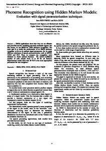
used for the transition matrices are known to be conservative since they include information on all states. Data and Analyses Dale et al. (17, 18) provide a description of the area investigated, which is on Coomera Island, Queensland (S27o 51', E153o 33') (Figure 1). The area is a major breeding site for mosquitoes, particularly Ochlerotatus vigilax (Skuse) which is a vector for alphaviruses such as Ross River Fever and Barmah Forest virus. Part of the area has been treated by runnelling to reduce mosquito numbers. Runnelling consists of linking isolated mosquito larval habitats to the tidal source via shallow ( 0.08 and >0.05 level, dependent analysis (key as in Figure 3).

20

Figure 1. Location of study area

21

Figure 2. Differences between the Independent and Dependent analyses (Values are mean values in the Dependent analysis minus the mean values in the Independent analysis (data as in Table I)

Mean number of Sporobolus 10 0 -10 0

1

2

3

4

5

6

7

8

9

7

8

9

7

8

9

8

9

Mean height of Sporobolus (mm) 10 0 -10 0

1

2

3

4

5

6

Mean number of Sarcocornia 10 0 -10 0

1

2

3

4

5

6

Mean size of Sarcocornia (mm) 10 0 -10 0

1

2

3

4

State

5

6

7

Figure 3. Linkages in terms of change at the P => 0.10, dependent analysis. Sporobolus: tall medium, short Sarcocornia: large, medium, small Density high, medium, low: No of symbols 3,2,1

P of remaining in same state P => .25 State

P> .10 < .25 (.08)

.69

.72

.52 State 7

State 1

State 6 .12

.15 .14

.44

.16

.49

State 9

State 3

.29

State 8 .70

.32

.43 .15 State 0 .93

State 2

State 4 .82

.10

.25

State 5 .76

Figure 4. Linkages at the > 0.08 and >0.05 level, dependent analysis .06

.08

.72

.69 .08

.52

State 7

State 1

State 6

.09 .15

.12

.08 .14

.07

State 9

.49

.44

.05

.05

.08

.16 State 3

State 8 .07

.32

.70

.29 .43 .05

State 0

.09

State 2

.15

State 4 .82

.93 .10

.25

.05

.05

P=> 0.05 P=> 0.08 P=> 0.10

State 5 .76