c Soudeh Ghorbani Khaledi et al. ⃝
University of Toronto SNL Technical Report TR10-SN-UT-07-10-21.
Using Memory and Random Sampling for Load Balancing in High-radix Switches Soudeh Ghorbani Khaledi, Yashar Ganjali
Amin Firoozshahian
Department of Computer Science, University of Toronto {soudeh, yganjali}@cs.toronto.edu
Hicamp Systems Inc.
[email protected]
Abstract—Dramatic increase in the size of communication networks as well as huge growth in data transmission rates have made designing high performance switches an essential part of building any interconnection network. Recent advances in fabrication technology have significantly increased the number of input and output ports in network switches. An interesting problem in designing such switches is how to balance the load among output ports of a switch when using adaptive routing algorithms. This problem is important for example in case of Clos networks and multi-stage load balanced switches; in the first stage of such a network/switch, packets from any input can be routed to any output port. Therefore, the decision of which output port to send the packets makes an important difference in the balance of the load in output ports and thus, in the throughput of the whole network. In practice, comparing the entire set of output queues to identify the best output port to direct a packet is prohibitively complex in the context of switches with a large number of ingress/egress ports (known as high-radix switches). In this paper we evaluate randomized schemes for balancing the load in such switches, both theoretically and via simulation. We prove that, despite being simple to implement, scheduling policies based on random sampling cannot guarantee stability when service rates are unequal. We also prove that simply adding one unit of memory to save the identity of least loaded queues in addition to few random samples can solve this problem: if no input port is oversubscribed, 100% throughput is achieved. We also present an extensive set of simulations to study the load distribution under different randomized scheduling algorithms with and without memory. We find that using as few as 2 or 3 random samples and one memory unit can result in balanced load in output queues regardless of low or high input loads and without any need for extra speedup.
2nd Stage
1st Stage
Fig. 1.
3rd Stage
Load balancing in multi-stage switches/Clos networks.
work switches that are very attractive substitutes for crossbar switches since they have fewer cross-points than a complete crossbar and therefore scaling them is much easier. Although Clos networks were first designed for circuit switches, they have been widely used in packet switching networks because of their nice properties like scalability, path diversity, low diameter, and their simple structure. Parallel packet switch (PPS) architectures [2], Distributed Switch Architecture (ADSA) [3], and load balanced Birkhoff-von Neuman switches [4] are other examples of multi-stage architectures in which arriving traffic is demultiplexed over lower speed switches, switched to the correct output port, and then recombined before leaving the system. A critical issue to be addressed in distributed switch architectures is the design of simple, fast and efficient loadbalancing scheduling algorithms for the first stage switches, so that they can balance the load by distributing the incoming packets evenly among the ports of the middle stage. The middle stage switches, then, route packets to their corresponding destination ports. As an example, let us consider a packet p going from input port i to output port j. The switch in the first stage which is connected to the input port i can route the packet to any of the middle stage switches. No matter which middle-stage switch receives the packet p, it can route it to the switch in the third stage connected to the output port j. Since there are k middle stage switches, the switch has a path diversity of k. We note that the path from any middle stage switch to the output port is unique (Figure 1(left)). Clearly, performance of a multistage switch architecture highly depends on how packets are routed, i.e. which middle stage switch is used to route each packet. If choosing the
I. I NTRODUCTION The size of communication networks and data transmission rates are constantly increasing. This makes designing high performance switches a must in building any interconnection network. In designing such switches, there are two main issues which need to be addressed: First, due to higher data transmission rates the time available for making routing decisions for each individual packet is very short. Therefore, routing decisions must be made very fast. Second, large networks require high-radix switches, i.e., switches with many input/output ports. Coordination among all the ports in such a switch is very costly in terms of complexity and cycle time. To remedy this situation the switching task can be parallelized by using multi-stage architectures that use lower speed and/or smaller switches operating independently and in parallel. Clos networks [1] are classical example of multi-stage net1
University of Toronto SNL Technical Report TR10-SN-UT-07-10-21.
1 (1,0) (1,1) (1,2)
0.9 0.8 0.7 0.6 0.5 0.4 0.3 0.2 0.1 0
0
10 20 30 40 50 60 70 Standard Deviation of the Occupancy of Output Queues
80
(a) d=1, m=0,1,2, 256*256 Switch 1 (2,0) (2,1) (2,2)
0.9 0.8 0.7 0.6 0.5 0.4 0.3 0.2 0.1 0
0
0.2 0.4 0.6 0.8 1 1.2 1.4 1.6 Standard Deviation of the Occupancy of Output Queues
1.8
(b) d=2, m=0,1,2, 256*256 Switch 1 (3,0) (3,1) (3,2)
0.9 0.8 0.7 0.6 0.5 0.4 0.3 0.2 0.1 0
0
0.1 0.2 0.3 0.4 0.5 0.6 0.7 Standard Deviation of the Occupancy of Output Queues
0.8
(c) d=3, m=0,1,2, 256*256 Switch Fig. 2. CDF of Standard Deviation of Output Queues’ Occupancy over Time for (d,m) Policies for Heavy Traffic and No Speedup For a 256*256 Switch.
2
middle stage is done inappropriately and too many packets are forwarded towards the same switch in the middle stage, the throughput of the network is reduced because of the congestion in the middle stage switch. To avoid this problem, each switch in the first stage of the network must try to distribute the load evenly on its output ports (Figure 1(right)). If all switches in the first stage can balance the load among their outgoing ports, the total load will be balanced in the middle stage and the throughput of the whole network is maximized. Note that if the service rate is identical for all the output ports, a simple round robin approach could achieve balanced load. Hence, we address the more challenging case where the service rates can vary among the output ports. To have perfect load balancing, there are two intertwined problems to solve. First, each input port needs to choose among a large list of output ports (for N ports, this is of time complexity O(N )). Second, we need an explicit or implicit coordination mechanism among all input ports to avoid all inputs directing their packets to the same output, as this leads to huge bursts and load imbalance in the network. To mitigate the cost of comparing the length of all output queues and avoid communication overhead, randomized version of scheduling might be considered: whenever a packet is arrived at any input port, it is assigned to the least loaded of d randomly chosen output queues, where d ≪ N . The classic load balancing problem in the literature (usually referred to as the supermarket models), considers a single input and many output queues as opposed to multiple inputs in our case. For that problem, it is well-known that with a small amount of choice d = 2 load balancing performance greatly improves over random placement d = 1 [5]. However, as we prove in Theorem 1 in Section 2, in our problem, i.e., in the switches under Bernoulli i.i.d. packet arrival processes for admissible traffic and when no input port is oversubscribed, scheduling by using only randomization can lead to instability. This problem, alas, cannot be resolved by increasing the number of samples: even for d = O(N ), where N in the number of outputs; there exists admissible traffic for which the system becomes unstable, unless d = N . On the positive side, we show that there is a simple way around this problem to guarantee stability. We theoretically prove that deploying a single unit of memory for each input port in which that port saves the identity of the output port with the shortest queue length from the previous time slots makes the system stable. We also present simulations that show random sampling with memory leads to nearly perfect load balance in system and can improve the performance of the system, e.g., it decreases the average and standard deviation of the occupancy of output queues. Our simulations show that regardless of the input load (light or heavy) and independent of the speedup of output queues (how many packets they can receive in each time slot) nearly perfect load balancing and acceptable latency is achievable with using very small number of samples, e.g., d = 2 or 3, and a single unit of memory for each input port. The organization of the paper is as follows. In Section
University of Toronto SNL Technical Report TR10-SN-UT-07-10-21.
II. L OAD BALANCING IN HIGH - RADIX SWITCHES
1 (1,0) (1,1) (1,2)
0.9 0.8 0.7 0.6 0.5 0.4 0.3 0.2 0.1 0
3
0
10
20 30 40 50 Avg. of the Occupancy of Output Queues
60
70
(a) d=1, m=0,1,2, 256*256 Switch 1 (2,0) (2,1) (2,2)
0.9 0.8 0.7 0.6 0.5 0.4
We consider an N × N combined input output queued switch with FIFO queues in which the arrivals are independent i.e., arrivals at each input are independent and identically distributed(i.i.d) and arrival processes at each input are independent of arrivals at other inputs. We further assume that arriving packets are of fixed and length. ∑equal ∑N Traffic is also N assumed to be admissible, i.e., i=1 δi ≤ i=1 µi , where δi is the arrival rate to input port i (1 ≤ i ≤ N ) and µj is the service rate of output queue j (1 ≤ j ≤ N ). (d, m) Scheduling Policy: We consider randomized scheduling that at each time slot, every input port chooses d random outputs out of possible N queues, finds the queue with minimum occupancy between these d samples and m least loaded samples from previous time slot, and routes its packet to it. At the end of each time slot, an input port will update the content of its m memory units with the identity of the least loaded output queues. In case of the contention for any given output port, that port will randomly choose K of the input ports, where 1 ≤ K ≤ N , and other input ports will be blocked. Such policies will be called (d, m) policies.
0.3 0.2
A. Load balancing using random sampling without memory
0.1 0
0
0.5
1 1.5 2 2.5 3 3.5 Avg of the Occupancy of Output Queues
4
4.5
(b) d=2, m=0,1,2, 256*256 Switch 1 (3,0) (3,1) (3,2)
0.9 0.8 0.7 0.6 0.5 0.4 0.3 0.2 0.1 0
0
0.2
0.4 0.6 0.8 1 1.2 1.4 Avg. of the Occupancy of Output Queues
1.6
1.8
(c) d=3, m=0,1,2, 256*256 Switch Fig. 3. CDF of Avg. of Output Queues’ Occupancy over Time for (d,m) Policies for Heavy Traffic and No Speedup For a 256*256 Switch.
2, the model employed for the theoretical analysis of the system and random policies are described. We also prove that scheduling policies based only upon random samples are unstable. Moreover, for admissible i.i.d. arrival processes, stability is proved for (d, m) policies when m ≥ 1. In Section 3, we explain how the policies are evaluated. The setup, components and results of our simulation are also presented. We provide an overview of related work in Section 4. The paper concludes in Section 5.
First, we consider (d, 0) policy, i.e., the algorithm in which every input port chooses d random outputs out of possible N queues, finds the queue with minimum occupancy between them and routes its packet to it. By Theorem 1, we prove that such algorithm cannot guarantee stability. Theorem 1: For unequal service rates and admissible i.i.d. arrival processes, (d, 0) policy cannot guarantee stability for any arbitrary number of samples d, where d is less than the number of outputs. Proof: Let δi be the arrival rate to input port i, and µj be the service rate of output queue j. Now consider output queue N . For any input port, the probability that it chooses output queue N as a sample is Nd . So, maximum arrival rate to queue ∑N N is Nd × i δi . Thus, the minimum arrival rate to the rest N − 1 output queues is δN −1 =
N ∑ i
∑ ∑ d d × δi = δi × (1 − ). N N i i N
δi −
N
Clearly, if δN −1 is larger than the sum of the service rates of these N − 1 queues, the system will be unstable. It should be noted that the argument does not hold 1) when there are some restriction regarding the service rates, like when the service rates are equal. Or, 2) when d = N . These two special cases, however, are of little interest. Since the former opts out some admissible patterns of traffic, and the latter will nullify the benefit of randomization. The results of our experiments suggest that the system will perform well with d ≪ N .
University of Toronto SNL Technical Report TR10-SN-UT-07-10-21.
4
1
1 (1,0) (1,1) (1,2)
0.9 0.8
0.8
0.7
0.7
0.6
0.6
0.5
0.5
0.4
0.4
0.3
0.3
0.2
0.2
0.1
0.1
0
0
50
100 150 200 Max of the Occupancy of Output Queues
250
(1,0) (1,1) (1,2)
0.9
300
0
0
20
(a) d=1, m=0,1,2, 256*256 Switch 1 (2,0) (2,1) (2,2)
0.8
0.8 0.7
0.6
0.6
0.5
0.5
0.4
0.4
0.3
0.3
0.2
0.2
0.1
0.1
0
1
2 3 4 5 6 Max of the Occupancy of Output Queues
7
(2,0) (2,1) (2,2)
0.9
0.7
8
0
0
1 2 3 4 5 90th Percentile of the Occupancy of Output Queues
(b) d=2, m=0,1,2, 256*256 Switch
6
(b) d=2, m=0,1,2, 256*256 Switch
1
1 (3,0) (3,1) (3,2)
0.9 0.8
0.8 0.7
0.6
0.6
0.5
0.5
0.4
0.4
0.3
0.3
0.2
0.2
0.1
0.1
0
0.5
1 1.5 2 2.5 3 Max of the Occupancy of Output Queues
3.5
(3,0) (3,1) (3,2)
0.9
0.7
0
200
(a) d=1, m=0,1,2, 256*256 Switch
1 0.9
0
40 60 80 100 120 140 160 180 90th Percentile of the Occupancy of Output Queues
4
(c) d=3, m=0,1,2, 256*256 Switch Fig. 4. CDF of Max of Output Queues’ Occupancy over Time for (d,m) Policies for Heavy Traffic and No Speedup For a 256*256 Switch.
0
0
0.2
0.4 0.6 0.8 1 1.2 1.4 1.6 1.8 90th Percentile of the Occupancy of Output Queues
2
(c) d=3, m=0,1,2, 256*256 Switch Fig. 5. CDF of 90th Percentile of Output Queues’ Occupancy over Time for (d,m) Policies for Heavy Traffic and No Speedup For a 256*256 Switch.
University of Toronto SNL Technical Report TR10-SN-UT-07-10-21.
5
B. Load balancing using random sampling with memory It was shown that randomized policy cannot guarantee stability without using unit of memory. By Theorem 2, we prove that having only one sample and using a single memory for each input port ensures stability for all uniform and nonuniform independent arrival processes. Theorem 2: (1, 1) policy is stable for all admissible i.i.d. arrival processes. To prove that the algorithm is stable, using the result of Kumar and Meyn [6], we show that for an N × N switch scheduled using the (1, 1) policy, there is a negative expected single-step drift in a Lyapunov function, V. In other words, E[V (n + 1) − V (n)|V (n)] ≤ ϵV (n) + k,
1 0.9 0.8 0.7 0.6 0.5 0.4 0.3 0.2 (1,0) (1,1) (1,2)
0.1
where k > 0 and ϵ > 0. We do so by defining V (n) as:
0
0 5 10 15 20 25 30 35 40 45 Standard Deviation of the Occupancy of Output Queues For 64*64 Switches
(a) d=1, m=0,1,2, 64*64 Switch
V (n) = V1 (n) + V2 (n), 1
where
(2,0) (2,1) (2,2)
0.9
V1 (n) =
N ∑
0.8
V1,i (n),
i=1
0.7 0.6 0.5
V1,i (n) = (˜ qi (n) − q ∗ (n))2 ,
0.4 0.3
V2 (n) =
N ∑
0.2
qi2 (n).
i=1 ∗
And qk (n), q˜k (n) and q (n), respectively, represent the length of the k-th output queue, the length of the output queue chosen by the input i, and the length of the shortest output queue in the system under policy (1, 1) at time instance n. Details of the proof can be found in the Appendix.
0.1 0
0 0.2 0.4 0.6 0.8 1 1.2 1.4 Standard Deviation of the Occupancy of Output Queues For 64*64 Switches
(b) d=2, m=0,1,2, 64*64 Switch 1 (3,0) (3,1) (3,2)
0.9 0.8 0.7
III. S IMULATIONS Stability of (d, m) policies, where m > 0 is proved in the previous section. Performance of different (d, m) policies are evaluated via simulation for different settings with different traffic load and speedup. In order to evaluate these policies, a reference scheme, hereafter called ideal, is used in which each input port will check the queue length of all of the output ports, and chooses the shortest one to send its packet to. It is worth emphasizing that this is done in parallel i.e. input ports cannot choose the output ports based on the results of the decision made by any other input ports. Moreover, for ideal policy, it is also assumed that any output queue can receive packets from all the input ports during each time slot, so that there will be no contention for output ports. It should be noted, however, that large number of packets that might be destined to a single output port may cause the so called ideal policy not to perform literally ideal in all scenarios.
0.6 0.5 0.4 0.3 0.2 0.1 0
0 0.1 0.2 0.3 0.4 0.5 0.6 0.7 0.8 0.9 Standard Deviation of the Occupancy of Output Queues For 64*64 Switches
(c) d=3, m=0,1,2, 64*64 Switch Fig. 6. CDF of Standard Deviation of Output Queues’ Occupancy over Time for (d,m) Policies for Heavy Traffic and No Speedup For a 64*64 Switch.
University of Toronto SNL Technical Report TR10-SN-UT-07-10-21.
A. Setup 1) Components: To keep the simulation setup simple, we have chosen to model only one node of the Clos network. Each node is an N × N combined input output queue switch. For the simulation, we ran the experiments on 256 × 256 and 64 × 64 switches. Each node contains an arbitrator, which decides which input queues have the highest priority when contending for an output port. In the experiments, these queues are chosen randomly. The switch fabric in each node is a crossbar that routes packets from the input queues to the output queues. This is done in parallel for all input ports. the router in the node decides which output port to send the packet to for every packet that is at the head of the input queues. We consider time to be slotted and that packets can arrive at the switch at the beginning of each time slot. Furthermore, we assume that at most one packet arrives at an input port and at most one packet departs from an output port during each time slot. Number of packets that can enter an output queue is also limited considering the speedup as explained in Speedup Section. Packets may have to wait at an input port if they lose the contention for the output port they choose, and may have to wait at an output port before departing. We also consider the capacity of input and output buffers to be infinitive. 2) Simulated Traffic: We assume that sum of arrival rates is smaller or equal to sum of service rates, and no input port is oversubscribed. For evaluating the policies, we consider 2 cases: when the system is heavily loaded, e.g., avg(δi )/avg(µj ) = 0.98, and when the system is lightly loaded, avg(δi )/avg(µj ) = 0.5, where δi and µj represents the arrival rate at input port i and service rate at output port j, respectively. We also assume that packets arriving to input ports have independent Bernoulli distributions. Since we are simulating a single node of a network, in order to get more realistic results we assign different service rates between zero and one. In a real system this is automatically done because of the backpressure from other switches in the system. Likewise, arrival processes are assumed to have unequal rates to mimic nonuniform traffic. 3) Speedup: In the randomized scheduling that we study, several input ports may compete for a specific output port. Our incentive for having faster internal fabrics actually stems from the need to be able to transfer more than a packet to each output port in a given time slot. Therefore, rather than enabling both input and output ports to respectively send and receive K packets during each time slot, which is feasible in switches with speedup of K, we are interested in the case that only output ports can receive up to K packets in each time slot, and akin to systems with no speedup, input ports are restricted to send out at most a single packet per time slot. Alternatively, by speedup of K, we mean that in each time slot, a given output port can grant permission to up to K of the input ports to destine their packets to it, while an input port can send out no more than a packet. Imposing the mentioned restriction on input ports causes us to only partially take advantage of potentials of switches with speedup. However, the results of
6
our experiments show that this restricted speedup still results in great improvement in system performance in terms of average latency of packets when the system is heavily loaded. In the experiments, we consider the case that the switch does not have speedup, and when it has speedup of 2. B. Simulation results 1) Heavy Traffic and No Speedup: Instability of (d, 0) policies makes exploiting memory inevitable. We dig closer into queue occupancy distributions when different number of memory units are used, and find that for small number of samples, d, taking advantage of a single memory unit considerably ameliorates balancing the load among output queues. As the number of samples increases, this effect gradually fades away. This is depicted in Figures 2, 3, 4, and 5 for d = 1, 2, 3, and for standard deviation, average, maximum and 90th percentile of output queues’s occupancy for a 256*256 switch, and in Figure 6 for standard deviation of output queues’ occupancy of a 64*64 switch. The figures suggest that the first memory unit causes the standard deviation, average, maximum, and 90th percentile of the policies with small number of sample to drop significantly which signals that balancing the load among the output ports is improved, but using the 2nd unit of memory does not have such strong effect. For other settings like light load or speedup of 2, and other values of d similar trend is observed. These results suggest that one unit of memory for each input port should be adequate. To figure out the appropriate number of samples, we measured statistical metrics of input and output queues’ occupancies for several (d, 1) policies, (256, 0) policy and ideal policy. Clearly, when the number of samples is equal to the number of input queues, 256 in this case, using memory will not alter the performance of the scheduling in any way, since at any time step the inputs will have all the information for determining the shortest output queues. Note that ideal and (256, 0) policies differ in the speedup of system (which is N for the former and 1 for the latter in this setting). As demonstrated in Figures 7 and 23 (a), the considered random policies all outperform the ideal policy by providing considerably lower average, standard deviation, max and 90th percentile of output queue occupancy. To have a better judgement of the random policies relative to each other, ideal policy is omitted from Figure 8 which demonstrates that nearly perfect load balancing in achievable with using as few as 2 or 3 samples and a single memory unit for each input port. In this setting, for random policies with several samples and m=1, average latency of packets will drop to nearly half of the latency for ideal policy. A number of these policies and their corresponding latency are mentioned in Table 1. 2) Heavy Traffic and Speedup of 2: Same experiment is repeated for the setting that speedup of switch is equal to 2, and very similar results are obtained: as Figures 9 and 23 (b) show the random policies all outperform the ideal policy. Among the random policies, as demonstrated by Figure 9, using only 2 or 3 samples and a single memory unit for each input port is sufficient to have balanced load and very small
University of Toronto SNL Technical Report TR10-SN-UT-07-10-21.
average output queue size. Note that although average and standard deviation of different policies have slightly increased compared to the setting with heavy load and no speedup, as Table 1 shows, average latency falls sharply to less than 15% of its corresponding value when the system does not have speedup for policies (2, 1) and (3, 1). Moreover, standard deviations are still very low. For (3, 1), for instance, standard deviation of the lengths of output queues is always under 0.8 which suggests that load is perfectly balanced among output ports. 3) Light Traffic and No Speedup: When the system is not heavily loaded, balancing the load is not that much of a challenge. As ρ = avg(δi )/avg(µi ) diminishes, ideal policy approaches the optimum case for balancing the load among outputs. Yet, having the speedup of N and comparing the length of all queues make it impractical. Measured metrics related to output queues’ occupancy in this case, depicted in Figures 11 and 23 (c) suggest that random policies will perform well in this setting as well when switch has no speedup. Also, as Table 1 shows, average latency for random policies is around 1/10 of its value for ideal case. 4) Light Traffic and Speedup of Two: Similar results are observed when the speedup of switch is 2, as shown by Figures 12 and 23 (d). In this case too, small number of samples and memory units guarantee low standard deviation of occupancy of output queues, and a relatively small number as the upper bound of queue occupancy. Average latency is only slightly diminished compared with the setting with no speedup. This should look trivial, considering that the switch is lightly loaded. The results suggests that when system is not heavily loaded, having speedup will not be of that much help in ameliorating the performance of switch. An Observation of Occupancy of Input Queues: For heavy traffic, when the system has no speedup, introducing memory increases the standard deviation, average, maximum and 90th percentile of input queues’ occupancy, as shown in Figures 13,14,15 and 16. However, as the number of samples increases, this increase in average and maximum occupancy gradually decreases. Intuitively, when memory is used for small number of samples, the probability that more input ports identify and target the same output ports increases. This will result in contention for a limited number of output ports, and since the switch does not have speedup, many of these input ports will lose the contention and be blocked. Consequently, the average and maximum input queues’ length increase in the system. However, these 2 numbers always remain under 100 and 275 packets, respectively, in our experiments (Figure 17). For heavy traffic when the switch has the speedup of 2, the average and maximum input queues’ occupancy are very small for small values of d, e.g., in (1,1), (2,1) and (3,1) policies (respectively, under 3 and 20 packets in all time for all these policies in our experiments, as shown by Figure 18). However, by increasing the number of samples these values increase. For light load (with or without speedup), as demonstrated in Figures 19 and 21, only for ideal policy input queues can become really large. As shown in zoomed Figures
7
20 and 22, all (d, m) policies (for small or large values of d) exhibit very small values for average and maximum input queues’ occupancy, with no considerable difference between these values for different ms and ds. In conclusion, in addition to the balanced load among output ports, (d, 1) policies with small number of samples, also provide vary small average and maximum input queues’ occupancy for light traffic, and for heavy traffic when the switch has the speedup of 2, and reasonably small values for heavy traffic in switches without speedup. IV. R ELATED W ORK The urgent need to build high speed switches has motivated many researchers to propose novel and high performance multi-stage switch architecture that scales up well. As an example of such attempts, Iyer et al. propose PPS architecture [2]. Iyer and McKeown show that the initial centralized approach used in PPS is impractical due to the large communication complexity that it requires [7]. They modify the PPS by allowing a small buffer, that runs at the line rate, in the multiplexer and the demultiplexer [7]. C.S. Chang et al.[4] have also proposed Birkhoff-von Neumann switch architecture with two-stage switching fabrics and one-stage buffering in which the 1st stage performs load balancing, while the 2nd stage is a Birkhoff-von Neumann input-buffered switch that performs switching for load balanced traffic. Although The on-line complexity of the switch is O(1), for the number of permutation matrices needed in their switch, the complexity is O(N ). ADSA architecture, proposed by Wang et al. [3] introduces a small communication overhead of log(P ) + 2log(N ) extra bits per cell in addition to the cell payload, where P is the number of parallel switch elements and N is the number of communication overhead. We believe that balancing the load in this context has a much simpler solution: randomization. While simplicity of implementation is clear, we proved the stability and evaluated the actual performance with simulation. The idea of using randomization and memory and the approach taken to theoretically prove the stability originate from previous work about load balancing. Randomization in standard load balancing problem is generally considers placing n balls into n bins by choosing d samples for each ball independently, uniformly at random and sequentially, and placing each ball in the least loaded of its chosen bins [8]. Apart from the ball and bin problem, another model, called supermarket model, is defined for dynamic settings in which arrivals occur according to a rate nλ(λ < 1) Poisson process at a bank of n independent rate exponential servers, with the ith server having service rate µi [8]. It is well established that for these problems, choosing a small number of samples significantly improves performance over random placement d = 1. Mitzenmacher et al. show that same performance gain can be achieved by deploying a small amount of memory [8]. Shah and Prabhakar introduce using a memory and prove the stability for the problems for (1, 1) policy [9]. Although supermarket problem is different
University of Toronto SNL Technical Report TR10-SN-UT-07-10-21.
TABLE I AVG . L ATENCY E XPERIENCED BY E ACH PACKET. Policy heavy traffic/sp=1 heavy traffic/sp=2 light traffic/sp=1 light traffic/sp=2
(1,1) 0.1710 0.0277 0.0142 0.0140
(2,1) 0.1648 0.0214 0.0140 0.0137
(3,1) 0.1637 0.0228 0.0138 0.0137
(100,1) 0.1674 0.0429 0.0139 0.0138
ideal/sp=256 0.2963 0.2963 0.1606 0.1606
from routing packets in high radix switches in that it has only a single arrival process and the arrivals will be served sequentially whereas in switches all arrivals in input ports are served simultaneously and in parallel, we take the same approach as Shah and Prabhakar [9] to show that the results similar to stability in supermarket problem hold valid in our switching problem as well. V. C ONCLUSION AND F UTURE W ORK In balancing the load in the output ports of a high-radix switch there are three main issues to be considered: First, in distributing the load from input ports to output queues, higher priorities must be given to shorter queues, i.e. more load must be forwarded to them. Second, the load-balancing scheme must not allow too many input ports to choose the same output queue since in this case blocking will occur. Finally, the load-balancing scheme must be very fast because of the high transmission rate of the switch and the large number of input/output ports. The randomized load-balancing methods studied in this paper have all of these properties. They are very fast since all the decisions are made based on the state of d randomly chosen output ports. They reduce the chance of blocking since output queues are chosen randomly and by choosing the shortest queue among these d random samples, they give higher priorities to shorter queues in the switch. We prove that only exploiting only random sampling can lead to instability, but also prove that using memory units for input ports can guarantee stability. Based on empirical results, we observe that using small values of samples, e.g., d = 2 or 3, and a single unit of memory for each input port results in perfect balance in the output queue lengths, and acceptable latency. The QoS guarantees that these policies may provide and their performance for different traffic patterns need to be investigated in future studies.
8
[6] P. Kumar and S. Meyn, “The randomness in randomized load balancing,” in Proc. of the 32nd IEEE Conference onDecision and Control, 15-17 1993, pp. 2730–2735 vol.3. [7] S. Iyer and N. McKeown, “Analysis of the parallel packet switch architecture,” IEEE/ACM Transactions on Networking, pp. 314–324, 2003. [8] M. Mitzenmacher, B. Prabhakar, and D. Shah, “Load balancing with memory,” Annual IEEE Symposium on Foundations of Computer Science, vol. 0, p. 799, 2002. [9] D. Shah and B. Prabhakar, “The use of memory in randomized load balancing,” in Proc. ISIT, 2002, p. 125.
A PPENDIX Theorem 1: (1, 1) policy is stable for all admissible i.i.d. arrival processes. Proof: Consider discrete instances of time when there is either an arrival or a departure, since these are the only times that the state of the system changes. We assume the speedup is K. We further assume at each time instance up to N packets arrive at the system according to N independent Bernoulli processes and the arrival rate to the input port i is δi (1 ≤ i ≤ N ). We denote by µi (1 ≤ i ≤ N ) the service rate of output port i (1 ≤ i ≤ N ). We assume that at most one packet can leave each queue at any given time instance (this assumption can be easily relaxed). Hence, the probability of having an arrival at any given time instant at δi∑ . Similarly, the probability that a input i is ∑N δ + N i=1 µi i=1 i departure occurs from output port i at any instant of time is µi ∑N ∑N . i=1 µi i=1 δi + Let qk (n), q˜k (n) and q ∗ (n) represent the length of the k-th output queue, the length of the output queue chosen by the input i and length of the shortest output queue in the system under policy (1, 1) at time instance n, respectively. If n is an arrival instant, then the probability that under (1, 1) policy input i chooses the shortest output queue, i.e., q˜i (n) = q ∗ (n), is at least 1/n. At each time instant, from up to N input ports that are contending for the same output port, at most K of them will be granted permission to direct their packets to that output. If by λi we refer to the arrival rate at output port i, then λi will be the of the ∑N ∑Nsummation arrival rate of these s input ports, and i=1 λi ≤ i=1 δi . The probability of having a packet forwarded to output port i is ∑N δ λ+i∑N µ . Moreover, by Lemma 1, proved in the i=1 i i=1 i appendix, we will show that N ∑
λi × qi (n) ≤
i=1
R EFERENCES [1] C. Clos, “A study of non-blocking switching networks,” Bell System Technical Journal, pp. 406–424, 1953. [2] S. Iyer, A. A. Awadallah, and N. McKeown, “Analysis of a packet switch with memories running slower than the line rate,” in Proc. IEEE INFOCOM, 2000, pp. 529–537. [3] W. Wang, L. Dong, and W. Wolf, “A distributed switch architecture with dynamic load-balancing and parallel input-queued crossbars for terabit switch fabrics,” in Proc. IEEE INFOCOM, 2002, pp. 352–361. [4] C.-S. Chang, D.-S. Lee, and Y.-S. Jou, “Load balanced Birkhoff-von Neumann switches, part I: one-stage buffering,” Computer Communications, vol. 25, no. 6, pp. 611–622, 2002. [5] M. Mitzenmacher, “The power of two choices in randomized load balancing,” IEEE Transactions on Parallel and Distributed Systems, vol. 12, pp. 1094–1104, 2001.
N ∑
δi × q˜i (n).
i=1
To prove that the algorithm is stable, using the result of Kumar and Meyn[6], we show that for an N × N switch scheduled using the (1, 1) policy, there is a negative expected single-step drift in a Lyapunov function, V. In other words, E[V (n + 1) − V (n)|V (n)] ≤ ϵV (n) + k, where k > 0 and ϵ > 0. Let V (n) be: V (n) = V1 (n) + V2 (n), where V1 (n) =
N ∑ i=1
V1,i (n),
University of Toronto SNL Technical Report TR10-SN-UT-07-10-21.
V1,i (n) = (˜ qi (n) − q ∗ (n))2 , V2 (n) =
N ∑
9 N ∑
i=1 δi
i=1
+
∑N i=1
qi2 (n).
i=1
1
∑N
i=1 δi
Since at most K packets can be enqueued at time instance n + 1 in q˜i when the speedup is K,
i=1 δi
And at most one packet can leave q ∗ at time instant n. So,
+
1
∑N
q˜i (n + 1) − q˜i (n) ≤ K. ∗
µi
∑N
+
(
N ∑
δi × (1 + 2
µi × (−2qi (n) + 1) =
i=1
1 +
∑N i=1
i=1
i=1 δi
[
N ∑
+
∑N i=1
1 δi )× ∑ ∑N N N i=1 δi + i=1 µi
2
i=1
∑ 1 1 × δi V1,i (n)+ ∑N ∑N N i=1 δi + i=1 µi i=1 N
i=1 δi
N ∑
1 1 × δi V1,i (n)+ ∑ ∑N N N δ + i=1 i i=1 µi i=1 N √ ∑ 2 V1,i (n) + N + N K.
2
+
i=1
µi
i=1 µi
×2
N ∑
i=1
µi (q ∗ (n) − qi (n)).
i=1
∑ 1 1 × δi V1,i (n)+ ∑N ∑N N i=1 δi + i=1 µi i=1
N √ ∑ V1,i (n)( ∑N
∑N
i=1 δi ∑N i=1 δi + i=1
∑N
i=1 δi
1 +
∑N i=1
δi
i=1 δi
∑N
E[V2 (n + 1) − V2 (n)|V2 (n)] =
i=1 δi
∑N
i=1
N
−
i=1
×(qi (n+1)−qi (n))(qi (n+1)−qi (n))+
µi
E[V (n + 1) − V (n)|V (n)] ≤
And for V2 ,
∑N
i=1
N N ∑ ∑ × 2q ∗ (n)( δi − µi )+
Thus,
i=1
λi
∑N
i=1 δi +
E[V1 (n + 1) − V1 (n)|V1 (n)] ≤
∑N
+
1
∑N
i=1
−
1
∑N
√ (2 V1,i (n) + K + 1)
So,
µi (q ∗ (n) − qi (n))].
E[V2 (n + 1) − V2 (n)|V2 (n)] ≤ ∑N i=1 δi + ∑N ∑N i=1 µi i=1 δi + √ ∑N 2 i=1 δi V1,i (n) + ∑N ∑N i=1 δi + i=1 µi
(2(˜ qi (n) − q ∗ (n)) + K + 1) ≤
N ∑
i=1
So,
N
−
N ∑ i=1
∑ 1 1 × δi (˜ qi (n) − q ∗ (n))2 + − ∑N ∑N N i=1 δi + i=1 µi i=1 N ∑
×
N N ∑ ∑ 2qi∗ (n)( δi − µi )+ i=1
((˜ qi (n + 1) − q ∗ (n + 1))2 − (˜ qi (n) − q ∗ (n))2 ) ≤
µi
√ δi × (1 + 2 V1,i )+
i=1
i=1
i=1
i=1
δi × ((˜ qi (n + 1) − q ∗ (n + 1))2 − (˜ qi (n) − q ∗ (n))2 )+
(1 −
×
i=1
1
∑N
N ∑
µi
N N ∑ ∑ √ V1,i + 2q ∗ (n)) + µi − 2 µi qi (n)) =
1 1 × ∑ ∑N N N i=1 δi + i=1 µi
i=1
µi
δi × (2˜ qi (n) + 1)+
i=1
N ∑
i=1 δi
E[V1 (n + 1) − V1 (n)|V1 (n)] =
N ∑
µi
∑N
Now consider:
N ∑
i=1
i=1
−q (n + 1) + q (n) ≤ 1. q˜i (n + 1) − q ∗ (n + 1) ≤ q˜i (n) − q ∗ (n) + K + 1.
N ∑
∑N
∑N
∗
Therefore,
×(qi (n+1)−qi (n))(qi (n+1)−qi (n)) =
µi
µi
µi
+
∑N i=1
µi
+ 1)+
+ N + N K+
N N ∑ ∑ × 2q ∗ (n)( δi − µi )+ i=1
i=1
University of Toronto SNL Technical Report TR10-SN-UT-07-10-21.
1
∑N
i=1 δi
+
∑N i=1
×2
µi
N ∑
10
µi (q ∗ (n) − qi (n)).
i=1
Hence, E[V (n + 1) − V (n)|V (n)] ≤ ∑N ∑N N ∑ −N ( i=1 δi + i=1 µi ) × δi i=1
(
)2 √ (V1,i ) δi − ( ∑N + 1) ∑N ∑N ∑N N ( i=1 δi + i=1 µi ) i=1 δi + i=1 µi ∑N ∑N ∑N δi i=1 δi i=1 µi + N + 3N + +(N + 1) ∑N i=1 ∑N ∑N i=1 δi i=1 µi i=1 δi δi
1
N K + ∑N
i=1 δi
1
+ ∑N
i=1 δi +
+
∑N i=1
∑N
i=1 µi
µi
N N ∑ ∑ × 2q ∗ (n)( δi − µi ) i=1
×2
N ∑
N(
δi
i=1 δi
δi
Bi = ∑N
i=1 δi +
+
µi (q ∗ (n) − qi (n)).
N
∑N
∑N i=1
∑N
µi
+1
µi
µi
+
+ 3N + N K
Ai ≥ 0 and Bi ≥ 0 and C ≥ 0 And, E[V (n + 1) − V (n)|V (n)] ≤ √ N ∑ V1,i Bi −( − 2 )2 + C (I) A A i i i=1 + ∑N
i=1 δi
+ ∑N
+ 1
i=1 δi +
∑N i=1
∑N
N N ∑ ∑ × 2q (n)( δi − µi ) (II) ∗
µi
i=1 µi
i=1
×2
So,
N ∑
λi × qi (n) ≤
N ∑
i=1
µi (q ∗ (n) − qi (n)) (II)
i=1
The following upper bounds are easily obtained: (I) ≤ C (II) ≤ 0, since the traffic is admissible. (III) ≤ 0, by definition of q ∗ (n). Suppose that V (n) is very large. If V1 (n) is very large, (I) will be negative, from which E[V (n + 1) − V (n)|V (n)] < −ϵ1 for V1 (n) > L1 follows. Otherwise, if V1 (n) is not very large but V (n) is, then V2 (n) should be very large which implies that length of some output queue, qi (n), is very large. If q ∗ (n) is not very large, then (III) will be less than −C which is a bounded constant. If q ∗ (n) is also
ρi,j × q˜j (n).
N ∑ N ∑
ρi,j × q˜j (n).
i=1 j=1
But since the input ports can compete for only a single output port at a time, the term ρi,j can be non-zero only for at most N pairs of (i, j). It follows that ρi,j × q˜j (n) =
i=1 j=1
Then,
1
N ∑ j=1
µi )
i=1
i=1 δi ∑N i=1 δi i=1
i=1 δi i=1 ∑N δ i=1 i
λi × qi (n) ≤
N ∑ N ∑
∑N
C = (N + 1) ∑N ∑N
It immediately follows that
i=1
i=1
∑N
∑N ∑N Lemma 1: ˜i (n). i=1 λi × qi (n) ≤ i=1 δi × q Proof: Let us define ρi,j { δj input j chooses output i ρi,j = 0 otherwise
i=1
So if we define Ai =
large, then (II) will be less than −C. In both cases, it follows that E[V (n+1)−V (n)|V (n)] < −ϵ2 for V2 (n) > L2 . Hence, there exist L and ϵ such that E[V (n + 1) − V (n)|V (n) is very large] < −ϵ for V (n) > L.
So,
N ∑ i=1
λi × qi (n) ≤
N ∑
δi × q˜i (n).
i=1 N ∑ i=1
δi × q˜i (n).
University of Toronto SNL Technical Report TR10-SN-UT-07-10-21.
1
11
1 (1,1) (2,1) (3,1) (20,1) (100,1) (256,0) ideal
0.9 0.8 0.7 0.6
0.9 0.8 0.7 0.6
0.5
0.5
0.4
0.4
0.3
0.3
0.2
0.2
0.1
0.1
0
0
10
20 30 40 50 Avg. of the Occupancy of Output Queues
60
70
0
(1,1) (2,1) (3,1) (20,1) (100,1) (256,0) 0
0.2
0.4 0.6 0.8 1 Avg. of the Occupancy of Output Queues
(a) 1
1 0.9
0.8
0.8
0.7
0.7
0.6
0.6
0.5
0.5
0.4
0.4 (1,1) (2,1) (3,1) (20,1) (100,1) (256,0) ideal
0.3 0.2 0.1
0
10 20 30 40 50 Standard Deviation of the Occupancy of Output Queues
(1,1) (2,1) (3,1) (20,1) (100,1) (256,0)
0.3 0.2 0.1
60
0
0
0.1 0.2 0.3 0.4 0.5 0.6 Standard Deviation of the Occupancy of Output Queues
(b) 1 (1,1) (2,1) (3,1) (20,1) (100,1) (256,0) ideal
0.8 0.7 0.6
0.9
0.7 0.6 0.5
0.4
0.4
0.3
0.3
0.2
0.2
0.1
0.1
0
20
40 60 80 100 120 Max of the Occupancy of Output Queues
140
(1,1) (2,1) (3,1) (20,1) (100,1) (256,0)
0.8
0.5
160
0
0
0.5
1 1.5 2 Max of the Occupancy of Output Queues
(c)
2.5
3
(c)
1
1 (1,1) (2,1) (3,1) (20,1) (100,1) (256,0) ideal
0.9 0.8 0.7 0.6
0.8 0.7 0.6 0.5
0.4
0.4
0.3
0.3
0.2
0.2
0.1
0.1
0
20 40 60 80 100 120 90th Percentile of the Occupancy of Output Queues
(1,1) (2,1) (3,1) (20,1) (100,1) (256,0)
0.9
0.5
0
0.7
(b)
1 0.9
0
1.4
(a)
0.9
0
1.2
140
0
0
0.2
0.4 0.6 0.8 1 1.2 1.4 1.6 1.8 90th Percentile of the Occupancy of Output Queues
2
(d)
(d)
Fig. 7. CDF of (a) Avg., (b) Standard Deviation, (c) Max and (d) 90th Percentile of Output Queues’ Occupancy Over Time for Heavy Traffic and No Speedup for (d,m) Policies and ideal policy in a 256*256 Switch.
Fig. 8. Zoomed CDF of (a) Avg., (b) Standard Deviation, (c) Max and (d) 90th Percentile of Output Queues’ Occupancy Over Time for Heavy Traffic and No Speedup for a 256*256 Switch.
University of Toronto SNL Technical Report TR10-SN-UT-07-10-21.
1
12
1 (1,1) (2,1) (3,1) (20,1) (100,1) (256,0) ideal
0.9 0.8 0.7 0.6
0.8 0.7 0.6
0.5
0.5
0.4
0.4
0.3
0.3
0.2
0.2
0.1
0.1
0
0
10
20 30 40 50 Avg. of the Occupancy of Output Queues
(1,1) (2,1) (3,1) (20,1) (100,1) (256,0)
0.9
60
70
0
0
1
2 3 4 5 6 Avg. of the Occupancy of Output Queues
(a) 1
1 (1,1) (2,1) (3,1) (20,1) (100,1) (256,0) ideal
0.8 0.7 0.6
0.9 0.8 0.7 0.6
0.5
0.5
0.4
0.4
0.3
0.3
0.2
0.2
0.1
0.1
0
10 20 30 40 50 Standard Deviation of the Occupancy of Output Queues
60
0
(1,1) (2,1) (3,1) (20,1) (100,1) (256,0) 0
0.2 0.4 0.6 0.8 1 1.2 Standard Deviation of the Occupancy of Output Queues
(b) 1 (1,1) (2,1) (3,1) (20,1) (100,1) (256,0) ideal
0.8 0.7 0.6
0.9 0.8 0.7 0.6
0.5
0.5
0.4
0.4
0.3
0.3
0.2
0.2
0.1
0.1
0
20
40 60 80 100 120 Max of the Occupancy of Output Queues
140
160
0
(1,1) (2,1) (3,1) (20,1) (100,1) (256,0) 0
1
(c)
2
3 4 5 6 7 8 Max of the Occupancy of Output Queues
9
10
(c)
1
1 (1,1) (2,1) (3,1) (20,1) (100,1) (256,0) ideal
0.9 0.8 0.7 0.6
0.9 0.8 0.7 0.6
0.5
0.5
0.4
0.4
0.3
0.3
0.2
0.2
0.1
0.1
0
1.4
(b)
1 0.9
0
8
(a)
0.9
0
7
0
20 40 60 80 100 120 90th Percentile of the Occupancy of Output Queues
140
0
(1,1) (2,1) (3,1) (20,1) (100,1) (256,0) 0
1
2 3 4 5 6 7 8 90th Percentile of the Occupancy of Output Queues
9
(d)
(d)
Fig. 9. CDF of (a) Avg., (b) Standard Deviation, (c) Max and (d) 90th Percentile of Output Queues’ Occupancy Over Time for Heavy Traffic and Speedup of 2 for (d,m) Policies and ideal policy in a 256*256 Switch.
Fig. 10. Zoomed CDF of (a) Avg., (b) Standard Deviation, (c) Max and (d) 90th Percentile of Output Queues’ Occupancy Over Time for Heavy Traffic and Speedup of 2 for a 256*256 Switch.
University of Toronto SNL Technical Report TR10-SN-UT-07-10-21.
13
1
1
0.9
0.9
0.8
0.8
0.7
0.7
0.6
0.6
0.5
0.5
0.4
0.4 (1,1) (2,1) (3,1) (20,1) (100,1) (256,0) ideal
0.3 0.2 0.1 0
(1,1) (2,1) (3,1) (20,1) (100,1) (256,0) ideal
0
0.1
0.2 0.3 0.4 0.5 Avg. of the Occupancy of Output Queues
0.6
0.3 0.2 0.1
0.7
0
0
0.1
0.2 0.3 0.4 0.5 0.6 0.7 Avg. of the Occupancy of Output Queues
(a) 1
1 0.9
0.8
0.8
0.7
0.7
0.6
0.6
0.5
0.5
0.4
(1,1) (2,1) (3,1) (20,1) (100,1) (256,0) ideal
0.4 (1,1) (2,1) (3,1) (20,1) (100,1) (256,0) ideal
0.3 0.2 0.1
0
0.1 0.2 0.3 0.4 0.5 0.6 Standard Deviation of the Occupancy of Output Queues
0.3 0.2 0.1
0.7
0
0
0.1 0.2 0.3 0.4 0.5 0.6 0.7 Standard Deviation of the Occupancy of Output Queues
(b) 1
1 (1,1) (2,1) (3,1) (20,1) (100,1) (256,0) ideal
0.8 0.7 0.6
0.9 0.8 0.7 0.6
0.5
0.5
0.4
0.4
0.3
0.3
0.2
0.2
0.1
0.1
0
0.5
1 1.5 2 Max of the Occupancy of Output Queues
2.5
3
0
(1,1) (2,1) (3,1) (20,1) (100,1) (256,0) ideal 0
0.5
(c)
1 1.5 2 Max of the Occupancy of Output Queues
2.5
3
(c)
1
1
0.9
0.9
0.8
0.8
0.7
0.7
0.6
0.6
0.5
0.5
0.4
0.4 (1,1) (2,1) (3,1) (20,1) (100,1) (256,0) ideal
0.3 0.2 0.1 0
0.8
(b)
0.9
0
0.9
(a)
0.9
0
0.8
0
0.1
0.2 0.3 0.4 0.5 0.6 0.7 0.8 0.9 90th Percentile of the Occupancy of Output Queues
(1,1) (2,1) (3,1) (20,1) (100,1) (256,0) ideal
0.3 0.2 0.1
1
0
0
0.2
0.4 0.6 0.8 1 1.2 1.4 1.6 1.8 90th Percentile of the Occupancy of Output Queues
2
(d)
(d)
Fig. 11. CDF of (a) Avg., (b) Standard Deviation, (c) Max and (d) 90th Percentile of Output Queues’ Occupancy Over Time for Light Traffic and No Speedup for (d,m) Policies and ideal policy in a 256*256 Switch.
Fig. 12. CDF of (a) Avg., (b) Standard Deviation, (c) Max and (d) 90th Percentile of Output Queues’ Occupancy Over Time for Light Traffic and Speedup of 2 for (d,m) Policies and ideal policy in a 256*256 Switch.
University of Toronto SNL Technical Report TR10-SN-UT-07-10-21.
1
14
1 (1,0) (1,1) (1,2)
0.9 0.8
0.8
0.7
0.7
0.6
0.6
0.5
0.5
0.4
0.4
0.3
0.3
0.2
0.2
0.1
0.1
0
0
10
20 30 40 50 60 70 80 Standard Deviation of the Occupancy of Input Queues
(1,0) (1,1) (1,2)
0.9
90
0
0
10
(a) d=1, m=0,1,2
80
1 (2,0) (2,1) (2,2)
0.8
0.8 0.7
0.6
0.6
0.5
0.5
0.4
0.4
0.3
0.3
0.2
0.2
0.1
0.1
0
10 20 30 40 50 60 70 Standard Deviation of the Occupancy of Input Queues
(2,0) (2,1) (2,2)
0.9
0.7
80
0
0
10
(b) d=2, m=0,1,2
20 30 40 50 Avg. of the Occupancy of Input Queues
60
70
(b) d=2, m=0,1,2
1
1 (3,0) (3,1) (3,2)
0.9 0.8
0.8 0.7
0.6
0.6
0.5
0.5
0.4
0.4
0.3
0.3
0.2
0.2
0.1
0.1
0
10 20 30 40 50 60 70 Standard Deviation of the Occupancy of Input Queues
(3,0) (3,1) (3,2)
0.9
0.7
0
70
(a) d=1, m=0,1,2
1 0.9
0
20 30 40 50 60 Avg. of the Occupancy of Input Queues
80
(c) d=3, m=0,1,2 Fig. 13. Effect of Memory on CDF of Standard Deviation of Input Queues’ Occupancy over Time for (d,m) Policies for Heavy Traffic and No Speedup For 256*256 Switches.
0
0
10
20 30 40 50 Avg. of the Occupancy of Input Queues
60
70
(c) d=3, m=0,1,2 Fig. 14. Effect of Memory on CDF of Avg. of Input Queues’ Occupancy over Time for (d,m) Policies for Heavy Traffic and No Speedup For 256*256 Switches.
University of Toronto SNL Technical Report TR10-SN-UT-07-10-21.
1
15
1 (1,0) (1,1) (1,2)
0.9 0.8
0.8
0.7
0.7
0.6
0.6
0.5
0.5
0.4
0.4
0.3
0.3
0.2
0.2
0.1
0.1
0
0
50
100 150 200 Max of the Occupancy of Input Queues
250
300
(1,0) (1,1) (1,2)
0.9
0
0
50 100 150 200 90th Percentile of the Occupancy of Input Queues
(a) d=1, m=0,1,2
(a) d=1, m=0,1,2
1
1 (2,0) (2,1) (2,2)
0.9 0.8
0.8 0.7
0.6
0.6
0.5
0.5
0.4
0.4
0.3
0.3
0.2
0.2
0.1
0.1
0
50
100 150 200 Max of the Occupancy of Input Queues
250
300
(2,0) (2,1) (2,2)
0.9
0.7
0
0
0
20
(b) d=2, m=0,1,2
40 60 80 100 120 140 160 90th Percentile of the Occupancy of Input Queues
180
200
(b) d=2, m=0,1,2
1
1 (3,0) (3,1) (3,2)
0.9 0.8
0.8 0.7
0.6
0.6
0.5
0.5
0.4
0.4
0.3
0.3
0.2
0.2
0.1
0.1
0
50
100 150 200 Max of the Occupancy of Input Queues
250
300
(c) d=3, m=0,1,2 Fig. 15. Effect of Memory on CDF of Max of Input Queues’ Occupancy over Time for (d,m) Policies for Heavy Traffic and No Speedup For 256*256 Switches.
(3,0) (3,1) (3,2)
0.9
0.7
0
250
0
0
20
40 60 80 100 120 140 160 90th Percentile of the Occupancy of Input Queues
180
200
(c) d=3, m=0,1,2 Fig. 16. Effect of Memory on CDF of 90th Percentile of Input Queues’ Occupancy over Time for (d,m) Policies for Heavy Traffic and No Speedup For 256*256 Switches.
University of Toronto SNL Technical Report TR10-SN-UT-07-10-21.
1
16
1 (1,1) (2,1) (3,1) (20,1) (100,1) (256,0) ideal
0.9 0.8 0.7 0.6
0.8 0.7 0.6
0.5
0.5
0.4
0.4
0.3
0.3
0.2
0.2
0.1
0.1
0
0
10
20 30 40 50 Avg. of the Occupancy of Input Queues
60
(1,1) (2,1) (3,1) (20,1) (100,1) (256,0) ideal
0.9
70
0
0
2
4
(a) 1
0.7 0.6
0.9 0.8 0.7 0.6
0.5
0.5
0.4
0.4
0.3
0.3
0.2
0.2
0.1
0.1
0
10
20 30 40 50 60 70 80 Standard Deviation of the Occupancy of Input Queues
90
0
(1,1) (2,1) (3,1) (20,1) (100,1) (256,0) ideal 0
5 10 15 20 25 Standard Deviation of the Occupancy of Input Queues
(b)
30
(b)
1
1
0.9
0.9
0.8
0.8
0.7
0.7
0.6
0.6
0.5
0.5
0.4
0.4 (1,1) (2,1) (3,1) (20,1) (100,1) (256,0) ideal
0.3 0.2 0.1
0
50
100 150 200 Max of the Occupancy of Input Queues
250
300
(1,1) (2,1) (3,1) (20,1) (100,1) (256,0) ideal
0.3 0.2 0.1 0
0
(c)
20
40 60 80 100 Max of the Occupancy of Input Queues
120
1
1 0.9
0.8
0.8
0.7
0.7
0.6
0.6
0.5
0.5
0.4
0.4 (1,1) (2,1) (3,1) (20,1) (100,1) (256,0) ideal
0.3 0.2 0.1
0
20
40 60 80 100 120 140 160 90th Percentile of the Occupancy of Input Queues
140
(c)
0.9
0
18
1 (1,1) (2,1) (3,1) (20,1) (100,1) (256,0) ideal
0.8
0
16
(a)
0.9
0
6 8 10 12 14 Avg of the Occupancy of Input Queues
180
200
(1,1) (2,1) (3,1) (20,1) (100,1) (256,0) ideal
0.3 0.2 0.1 0
0
10 20 30 40 50 60 90th Percentile of the Occupancy of Input Queues
70
(d)
(d)
Fig. 17. CDF of (a) Avg., (b) Standard Deviation, (c) Max and (d) 90th Percentile of Input Queues’ Occupancy Over Time for Heavy Traffic and No Speedup for (d,m) Policies and ideal policy in a 256*256 Switch.
Fig. 18. CDF of (a) Avg., (b) Standard Deviation, (c) Max and (d) 90th Percentile of Input Queues’ Occupancy Over Time for Heavy Traffic and Speedup of 2 for (d,m) Policies and ideal policy in a 256*256 Switch.
University of Toronto SNL Technical Report TR10-SN-UT-07-10-21.
17
1
1
0.9
0.9
0.8
0.8
0.7
0.7
0.6
0.6
0.5
0.5
0.4
0.4 (1,1) (2,1) (3,1) (20,1) (100,1) (256,0) ideal
0.3 0.2 0.1 0
(1,1) (2,1) (3,1) (20,1) (100,1) (256,0)
0
50
100 150 200 Avg. of the Occupancy of Input Queues
250
300
0.3 0.2 0.1 0
0
0.1
(a) 1
1 0.9
0.8
0.8
0.7
0.7
0.6
0.6
0.5
0.5
0.4
0.2 0.1
(1,1) (2,1) (3,1) (20,1) (100,1) (256,0)
0
50 100 Standard Deviation of the Occupancy of Input Queues
150
0.3 0.2 0.1 0
0
0.1 0.2 0.3 0.4 0.5 0.6 0.7 0.8 Standard Deviation of the Occupancy of Input Queues
(b)
0.9
(b)
1
1
0.9
0.9
0.8
0.8
0.7
0.7
0.6
0.6
0.5
0.5
0.4
(1,1) (2,1) (3,1) (20,1) (100,1) (256,0)
0.4 (1,1) (2,1) (3,1) (20,1) (100,1) (256,0) ideal
0.3 0.2 0.1
0
100
200 300 400 Max of the Occupancy of Input Queues
500
600
0.3 0.2 0.1 0
0
1
(c) 1
1 0.9
0.8
0.8
0.7
0.7
0.6
0.6
0.5
0.5
0.4
(1,1) (2,1) (3,1) (20,1) (100,1) (256,0) ideal
0.3 0.2 0.1
0
50
2 3 4 5 Max of the Occupancy of Input Queues
6
7
(c)
0.9
0
0.7
0.4 (1,1) (2,1) (3,1) (20,1) (100,1) (256,0) ideal
0.3
0
0.6
(a)
0.9
0
0.2 0.3 0.4 0.5 Avg. of the Occupancy of Input Queues
100 150 200 250 300 350 400 90th Percentile of the Occupancy of Input Queues
450
0.4 (1,1) (2,1) (3,1) (20,1) (100,1) (256,0)
0.3 0.2 0.1 0
0
0.1
0.2 0.3 0.4 0.5 0.6 0.7 0.8 90th Percentile of the Occupancy of Input Queues
0.9
1
(d)
(d)
Fig. 19. CDF of (a) Avg., (b) Standard Deviation, (c) Max and (d) 90th Percentile of Input Queues’ Occupancy Over Time for Light Traffic and No Speedup for (d,m) Policies and ideal policy in a 256*256 Switch.
Fig. 20. Zoomed CDF of (a) Avg., (b) Standard Deviation, (c) Max and (d) 90th Percentile of Input Queues’ Occupancy Over Time for Light Traffic and No Speedup for (d,m) Policies and ideal policy in a 256*256 Switch.
University of Toronto SNL Technical Report TR10-SN-UT-07-10-21.
18
1
1
0.9
0.9 (1,1) (2,1) (3,1) (20,1) (100,1) (256,0) ideal
0.8 0.7 0.6 0.5
0.7 0.6 0.5
0.4
0.4
0.3
0.3
0.2
0.2
0.1
0.1
0
0
50
100 150 200 Avg. of the Occupancy of Input Queues
250
300
(1,1) (2,1) (3,1) (20,1) (100,1) (256,0)
0.8
0
0
0.05
(a) 1
1 0.9
0.8
0.6 0.5 0.4
0.7 0.6 0.5 0.4
0.3
0.3
0.2
0.2
0.1
0.1
0
50 100 Standard Deviation of the Occupancy of Input Queues
150
0
0
0.1 0.2 0.3 0.4 0.5 0.6 Standard Deviation of the Occupancy of Input Queues
(b) 1
1 0.9 (1,1) (2,1) (3,1) (20,1) (100,1) (256,0) ideal
0.8 0.7 0.6 0.5
0.7 0.6 0.5 0.4
0.3
0.3
0.2
0.2
0.1
0.1
200 300 400 Max of the Occupancy of Input Queues
500
600
(1,1) (2,1) (3,1) (20,1) (100,1) (256,0)
0.8
0.4
100
0
0
0.5
(c)
1 1.5 2 2.5 3 Max of the Occupancy of Input Queues
3.5
4
(c)
1
1
0.9
0.9
0.8
0.8 (1,1) (2,1) (3,1) (20,1) (100,1) (256,0) ideal
0.7 0.6 0.5 0.4
0.7
0.5 0.4 0.3
0.2
0.2
0.1
0.1
0
50
100 150 200 250 300 350 400 90th Percentile of the Occupancy of Input Queues
450
(1,1) (2,1) (3,1) (20,1) (100,1) (256,0)
0.6
0.3
0
0.7
(b)
0.9
0
0.4
(1,1) (2,1) (3,1) (20,1) (100,1) (256,0)
0.8 (1,1) (2,1) (3,1) (20,1) (100,1) (256,0) ideal
0.7
0
0.35
(a)
0.9
0
0.1 0.15 0.2 0.25 0.3 Avg. of the Occupancy of Input Queues
0
0
0.1
0.2 0.3 0.4 0.5 0.6 0.7 0.8 90th Percentile of the Occupancy of Input Queues
0.9
1
(d)
(d)
Fig. 21. CDF of (a) Avg., (b) Standard Deviation, (c) Max and (d) 90th Percentile of Input Queues’ Occupancy Over Time for Light Traffic and Speedup of 2 for (d,m) Policies and ideal policy in a 256*256 Switch.
Fig. 22. Zoomed CDF of (a) Avg., (b) Standard Deviation, (c) Max and (d) 90th Percentile of Input Queues’ Occupancy Over Time for Light Traffic and Speedup of 2 for (d,m) Policies and ideal policy in a 256*256 Switch.
University of Toronto SNL Technical Report TR10-SN-UT-07-10-21.
1
19
1 (1,1) (2,1) (3,1) (20,1) (64,0) ideal
0.9 0.8 0.7
0.8 0.7
0.6
0.6
0.5
0.5
0.4
0.4
0.3
0.3
0.2
0.2
0.1
0.1
0
0
0 1 2 3 4 5 6 7 Standard Deviation of the Occupancy of Output Queues for 64*64 Switches
(1,1) (2,1) (3,1) (20,1) (64,0) ideal
0.9
0 1 2 3 4 5 6 7 Standard Deviation of the Occupancy of Output Queues for 64*64 Switches
(a)
(b)
1
1 (1,1) (2,1) (3,1) (20,1) (64,0) ideal
0.9 0.8 0.7
0.8 0.7
0.6
0.6
0.5
0.5
0.4
0.4
0.3
0.3
0.2
0.2
0.1
0.1
0
0
0 0.5 1 1.5 2 2.5 3 Standard Deviation of the Occupancy of Output Queues for 64*64 Switches
(c)
(1,1) (2,1) (3,1) (20,1) (64,0) ideal
0.9
0 0.2 0.4 0.6 0.8 1 1.2 1.4 Standard Deviation of the Occupancy of Output Queues for 64*64 Switches
(d)
Fig. 23. CDF of Standard Deviation of Output Queues’ Occupancy over Time for (a) Heavy Traffic and No Speedup, (b) Heavy Traffic and Speedup of 2, (c) Light Traffic and No Speedup, and (d) Light Traffic and Speedup of 2 for a 64*64 Switch.