[9] Donald A. Berry and Bernard W. Lindgren, âStatistics theory and. Methodsâ, 2nd ed., Duxbury Press, ITP, 1996. [10] John M. Gottman, âTime-series analysisâ, ...
1
Adaptive Random Sampling for Traffic Load Measurement Baek-Young Choi, Jaesung Park, Zhi-Li Zhang Department of Computer Science and Engineering University of Minnesota, MN, USA
Abstract— Traffic measurement and monitoring is an important component of network QoS management and traffic engineering. With high-speed Internet backbone links, efficient and effective packet sampling techniques for traffic measurement are not only desirable, but increasingly becoming a necessity. In this paper, we propose and analyze an adaptive random packet sampling technique for traffic load measurement. In particular, we address the problem of bounding sampling error within a prespecified tolerance level. We derive a relationship between the number of packet samples, the accuracy of load estimation and the squared coefficient of variation of packet size distribution. Based on this relationship, we propose a sampling technique that determines the minimum sampling probability adaptively according to traffic dynamics. Using real network traffic traces, we show that the proposed adaptive random sampling technique indeed produces the desired accuracy, while also yielding significant reduction in the amount of traffic samples, yet simple to implement.
I. I NTRODUCTION Traffic measurement and monitoring serve as the basis for a wide range of network QoS management and engineering tasks. With today’s high-speed links, however, inspecting every single packet traversing a link is extremely costly. It may significantly impact router performance depleting processing resources [15]. With off-board measurement devices, huge volumes of data are generated which can quickly exhaust storage space. Packet sampling has been suggested as a scalable alternative to address this problem. Both the Internet IETF working groups IPFIX (IP Flow Information Export) [1] and PSAMP (Packet Sampling) [2] have recommended the use of packet sampling. 1-out-of- , static systematic sampling is a popular sampling design employed in Cisco and Juniper routers [3], [4]. The foremost and fundamental question regarding sampling is its accuracy. This is especially pertinent in the Internet, where traffic is known to fluctuate frequently. Inaccurate packet sampling not only defeats the purpose of traffic measurement and monitoring, but worse, can lead to wrong decisions by network operators. Another important related question is the efficiency of packet sampling. Excessive oversampling should also be avoided for the measurement solution to be scalable. Therefore, it is important to control the accuracy of estimation so as to balance the trade-off between the utility and overhead of measurements. Given the dynamic nature of network traffic, static sampling does not always ensure the accuracy of estimation, and tends to oversample at peak periods when economy and timeliness are most critical.
In this paper we develop an adaptive random sampling technique for load change detection using sampled traffic measurement. Our adaptive random sampling technique differs from existing sampling techniques for traffic measurement in that it yields bounded sampling errors within a prespecified error tolerance level. Furthermore, the pre-specified error tolerance level allows us to control the performance of its application as well as the amount of packets sampled. The paper is devoted to the analysis and verification of the proposed adaptive random sampling technique for traffic load measurement. Our contributions are summarized as follows. We observe that sampling errors in estimating traffic load arises from dynamics of packet sizes and counts, and these traffic parameters vary over time. Consequently, static sampling (i.e., with a fixed sampling rate) cannot guarantee errors within a given error tolerance level. From our analysis, we find that the minimum required number of samples to bound sampling error within a given tolerance level is proportional ) of packet size to the squared coefficient of variation ( distribution. Using this relationship, we propose an adaptive random sampling technique that determines the (minimum) of packet sampling probability adaptively based on the size distribution and the packet count. More specifically, time is divided into (non-overlapping) observation periods (referred to as (time) blocks), and packets are sampled in each observation period. At the end of each block, in addition of to estimating the traffic volume of the block, the packet size distribution and the packet count of the block are calculated using the traffic samples. These traffic parameters of packet size distribution and are used to predict the the packet count of the next block, using an Auto-Regressive (AR) model. The sampling probability for the next block is then determined based on these predicted values and the given error tolerance level. The procedure is depicted in Figure 1. Using real network traffic traces, we show that the proposed adaptive random sampling technique indeed produces the desired accuracy, while at the same time yielding significant reduction in the amount of traffic samples. Before we leave this section, we would like to comment that in the context of traffic measurement and analysis, several sampling methods have been proposed and studied for various applications. Statistical sampling of network traffic was first evaluated in [5] for measuring traffic on the NSFNET backbone in the early 1990’s. Claffy et al. evaluated classical event and time driven static sampling methods to estimate statistics of distributions of packet size and inter-arrival time, and
���
���
���
���
2
4
x 10
sampled packets 4
Load
total packet count mk - 1 total sample count nk - 1
2
0
0
500
1000
1500
2000
2500
3000
3500
4000
4500
0 4 x 10
500
1000
1500
2000
2500
3000
3500
4000
4500
0
500
1000
1500
2000 2500 time (sec)
3000
3500
4000
4500
Avg. Pkt Size
300
packet arrivals
200 100 0
kth time block(B) Packet Count
(k-1)th time block(B)
~
estimate traffic volume Vk - 1 predict traffic parameters for next block
( SCVks- 1 , mk - 1 )
Fig. 1.
( SCˆ Vk , mˆ k )
Adaptive random sampling.
observed that event driven outperforms time driven approach. In [6], random packet sampling is used for evaluation of ATM end-to-end QoS such as cell transfer delay. Hash based sampling proposed in [11] employs the same hashing function at all links in a network to sample same set of packets at different links and to infer statistics on the spatial relations of the network traffic. In [8], a probabilistic packet sampling method is used to identify large flows. Each packet has to be inspected and its sampling probability is computed based on the packet size. A size-dependent flow sampling method proposed in [7] addresses the issue of reducing the bandwidth needed for the transmission of traffic measurements to a backoffice system for later analysis. For the purpose of usage-based charging, flows are probabilistically sampled depending on their sizes, assuming flow statistics are known a priori. None of these sampling techniques address the issue of bounding sampling errors in random packet sampling to reduce per-packet processing overhead under dynamic traffic conditions. The remainder of the paper is structured as follows. In Section II, we formally state the problem addressed in this paper. In Section III, the adaptive random sampling technique is described and analyzed. Experimental results with real network traffic traces are presented in Section IV. Section V concludes the paper. II. S AMPLING P ROBLEM FOR L OAD C HANGE D ETECTION In this section we first formulate the sampling problem for traffic load measurement. We then derive a lower bound on the number of samples needed to estimate the traffic load accurately within a given tolerance level. Based on this, we determine the sampling probability that is optimal in the sense that it guarantees the given accuracy with the minimum number of samples. We also discuss the limitations of static sampling under dynamic traffic conditions. A. Bounding Sampling Errors in Traffic Load Estimation Traffic load is the sum of the sizes of packets arriving during a certain time interval. Thus, traffic load is determined by both the number of packets and their sizes. In determining the traffic load, the variability of packet sizes is often overlooked and only packet count is considered. However, as noted in
2 1.5 1 0.5 0
Fig. 2.
Impact of packet size and packet count on traffic load (trace
).
[22], average packet size plays an important role in estimating the traffic load. Consider, for example, network traffic traces captured at University of Auckland [13] to US link. The time in Table II) series plot of the traffic loads of the traces ( is shown in the top row of Figure 2. The plot in the middle row shows the average packet sizes over time, while the plots in the bottom row show the packet counts over time. From Figure 2, we see that the increase in the traffic load around ���� sec is due to the increase in the packet size rather than the packet count. The example illustrates that the variation in packet sizes is an important factor in estimating the traffic load using sampling. In fact, we will show later that the variation in packet sizes is the key factor in determining the sampling rate and for controlling the accuracy of load estimation. Traffic loads is estimated from packets sampled during (nonoverlapping) observation periods of fixed length (see Figure 1). We refer to an observation period as a (load estimation) time block, or simply block. The length of a block is denoted by , which can be configured depending on the specific engineering purposes. We bound the sampling error in each block quantitatively. In the following we state the problem of bounding sampling errors in traffic load estimation formally.
�
� � �
packets arriving in a block, and Assume that there are be the size of the th packet. Hence the traffic load of let . To estimate the traffic load of the this block is � �� block, suppose we randomly sample , � , packets out of the packets. In other words, each packet has an equal to be sampled. Let � � , � � � , probability � denote the size of the th sampled packet. Then the traffic load can be estimated by � using the samples, where � is given by
�
�
� � �
�
�
�
�
�� � ��
� � � �
� �
� �� �
(1)
�
� ��
It can be shown that � is an unbiased estimator of , i.e., � � � � � �. The estimator can also be shown to be consistent, as � � when � .
��
�
�
�
�
�
� �
�� �
�� �
Our objective is to bound the relative error � � � within a prescribed error tolerance level given by two parameters � � �
� �
� � � �), i.e.,
��� �� � � �� � �� ��� � ��� � �
�
(2)
In other words, we want the relative error in traffic load estimation using random sampling to be bounded by with a high probability � � . Given this formulation of the bounded error sampling problem, the question is what is the minimum number of packets that must be sampled randomly so as to guarantee the prescribed accuracy. We address this question in the following subsection.
�
B. Optimal Sampling Probability and Limitations of Static Sampling From the central limit theorem of random samples1 [9], � �, the average of sampled data as the sample size approaches the population mean, regardless of distribution of population. Thus (2) can be rewritten as follows:
�
��� �� � � �� � �� ��� � ��� � � �
�
�
�
��
� � � � � ��� �
�
� � �� � �£ � � ��� � � � �� � � � � �
�
�
(4)
where � = � ��� ���� and �
� is the squared ) of the packet size distribution coefficient of variance ( in a block. Eq. (4) concisely relates the minimum number of packet samples to the estimation accuracy and the variability in packet sizes. In particular, it states the minimum required number of packet samples, £ , is linearly proportional to the squared coefficient of variance, , of the packet size distribution in a block. From (4) we conclude that the optimal sampling probability, £ , which samples the minimum required number of packets in a block, is given by ½
�
�
���
�
� �
�
£
£ � ��
(5)
� �
Hence, to attain the prescribed sampling accuracy � �, packets in a block must be sampled randomly with a probability at least £ . Note that to determine the optimal sampling probaof the packet size bility £ , we need to know the actual
0.01 50
100
150
200
250
50
100
150
200
250
50
100
200
250
0.3 0.2 0.1
3
2
1 150 time(300sec)
Fig. 3. Importance of adaptiveness: adaptive vs. static random sampling ( � �� � ���� ����), trace � .
�
distribution and the packet count in a block. Unfortunately, in practice these traffic parameters of a block are unknown to us at the time the sampling probability for the block must be determined. To circumvent this problem, in Section III we develop an AR (Auto-Regressive) model to predict these parameters of a block based on past sampled measurements of previous blocks. Before we proceed to present this model, (3)we would like to conclude this section by discussing the limitations of static sampling. Static sampling techniques such as “one-out-of-N” sampling are commonly employed in routers, as they are simple to implement. For example, Cisco’s Sampled NetFlow [3] samples one packet out of every IP packets for flow statistics.2 More generally, static random sampling technique randomly samples a packet with a fixed probability. Both techniques do not take traffic load dynamics into account, thus when applied to traffic load estimation, they cannot guarantee that the sampling error in each block falls within a prescribed error tolerance level. Furthermore, it is difficult to determine what is the appropriate fixed sampling probability (or the value for N in “one-out-ofN” sampling) to be used for all blocks. To help illustrate the importance of adjusting sampling probability to packet size variability, in Figure 3 we compare the optimal adaptive random sampling technique to the static random sampling technique using the Auckland trace � shown in Table II. To make fair comparison, the fixed sampling probability for the static random sampling technique is set such that the sampling fraction (i.e., the amount of sampled data) over the entire trace is the same as that under the optimal adaptive random sampling technique. The top plot in Figure 3 shows the optimal sampling probability used by the adaptive � ��� ) sampling technique over time (the block size as well as the fixed sampling probability used by the static random sampling. The middle plot shows the resulting relative errors by both sampling techniques. The bottom plot shows the of the packet sizes across the blocks. From the figure we see that when the variability of packet size distribution of a block is large, static random sampling
� �� �� � � �� ���� � �� � ��� � � � ���� � � � � � ��
where and are, respectively, the population mean and standard deviation of the packet size distribution in a block, and � � is the cumulative distribution function (c.d.f) of the standard normal distribution (i.e., � � ). Hence, to satisfy the given error tolerance level, the required number of packet samples must satisfy
�
0.02
SCV
�
adaptive random sampling static random samplig
0.03
abs. rel. error
(�
samplig probability
3
���
1 The requirement of samples being i.i.d (independent and identically distributed) for the condition of the theorem is achieved by random sampling from the common population. Recall that randomizing eliminates correlation. For example in [17], randomizing technique is used to destroy correlation for the purpose of investigating the impact of long range dependence on the queueing performance.
�
���
���
2 Though systematic sampling technique does not give any assessment of error, when the packet sizes are random in the arriving order, it simulates random sampling.
4
���
TABLE I N OTATION .
� �� ��� �� � � � �
��� of the population of �th block ��� of the samples of �th block predicted ��� of the samples of � th block minimum number of samples needed in � th block
predicted minimum number of samples needed in � th block actual number of samples in � th block actual number of packets in � th block predicted number of packets in � th block
tends to undersample packets, resulting in large estimation errors. On the other hand, when the variability of packet size distribution of a block is small, static random sampling tends to oversample packets, thereby wasting processing capacity and memory space of the measurement device. Moreover, the frequent oscillation between oversampling and undersampling of static random sampling causes undesirable increase in the variance of estimation errors. This example demonstrates that in order to ensure a desired accuracy in traffic load estimation while without resorting to unnecessary oversampling, packet sampling probability for each block must be adjusted in accordance with the traffic load dynamics. This is the essential idea behind our proposed adaptive random sampling technique. The key challenge remains to be addressed is how to determine the (optimal) sampling probability for each block without a priori of packet size knowledge of the traffic parameters – the distribution and packet count of a block. The next section is devoted to the analysis and solution of this problem.
In this section we present an AR (Auto-Regressive) model for predicting two key traffic parameters for traffic load estimaof packet size distribution and packet count of tion – the a block – using past (sampled) data from previous blocks. The AR model is justified by empirical studies using real network traffic traces. We also analyze the impact of the prediction errors and discuss how these errors can be controlled.
���
A. AR Model for Traffic Parameter Prediction The efficacy of prediction depends on the correlation among the past and future values of the parameters being predicted. We have analyzed many public-domain real network traffic traces, a subset of traces we studied is listed in Table II. We ’s of the packet sizes of two consecutive found that the blocks are strongly correlated; the same is also true for the packet counts, ’s, of two consecutive blocks. As an illustration, Figures 4(a) and 4(b) show, respectively, the scatter plots and of two consecutive blocks (the block size of � � ) using the trace in Table II. It is evident that and of two consecutive blocks are highly the values of correlated, in that the correlation coefficients are very close to �. In fact, there is a strong linear relationship between these values. The predictability may depend on the time scale (block size) of observation. We observed strong positive correlations to �� for long for a wide range of time scale from �
��� � ��� � � ��� ��� �
���
���
���
���
�
� ���
�
���
�
�
���
III. A DAPTIVE R ANDOM S AMPLING WITH B OUNDED E RRORS
���
to �� for short ( � ) traces [23]. As traces and � a further justification, we remark that the predictability of network traffic has also been studied by other researchers. For instance, in [16] the authors investigated the questions of how far into the future a traffic rate process can be predicted for a given error constraint. They showed that prediction works well for one step into the future, although it degrades quickly as the number of steps increases. In the context of our work, note that we only need to predict the traffic parameters for the next step (i.e., the next block). We employ an AR (Auto-Regressive) model for predicting and , as compared to other the traffic parameters time series models, the AR model is easier to understand and computationally more efficient. In particular, using the AR model, the model parameters can be obtained by solving a set of simple linear equations [10], making it suitable for online traffic load estimation. In the following we formally describe the AR model for the traffic parameter prediction. We first present an AR( ) model for predicting the of the next block using the of sampled packet sizes of the previous blocks. The notation used here and in the rest of this paper is summarized in Table I. Let be the of the packet sizes in the th block, and be the of the packet sizes randomly sampled in the th block. We can relate and as follows:
�
� �� ��
�
�
� �
��� ���
(6)
���
where denotes the error in estimating the actual the packet sizes using the random packet samples. Using the AR( ) model [10], can be expressed as
�
�
� �
� �
of
�� � �
��
� � ��� � �
��
(7)
�
where , � � , are the model parameters, and is the uncorrelated error (which we refer to as the prediction error). The error term follows a normal distribution with mean � and variance � � � � � ��� � . Here � is the lag- autocorrelation of ’s. The model parameters , �� , can be determined by solving a set of linear equations (8) in terms of past values of ’s, where � is a configurable parameter independent of , and is typically referred to as the memory size.
�
�
�
�
�
�
�
�
�
� �
��
�
�
�
��
! � � �
(8)
! �
� � � and � is lag- autocorrelation where � of the data. Using the above AR( ) model, at the end of the ( � �)th block, we predict the of the th block using values of the sampled packet sizes of the previous the blocks as follows:
�
� ���
���
�� �
�� � �
��
�
(9)
Combining (6), (7) and (9), we have
�� � � � � � �
(10)
5
8
12000
7 10000 6 8000
m(k)
SCV(k)
5
4
6000
3 4000 2 2000 1
0
0
1
2
3
4 SCV(k−1)
(a) SCV ( � � � ��
5
6
7
0
8
0
2000
� ������)
4000
6000 m(k−1)
8000
(b) Packet count ( � � � ��
10000
12000
� ������)
Relationship between past and future values of ��� and packet count.
Fig. 4.
0.25
0.12 estimation error prediction error total error 0.1
Given error tolerance level
0.2
0.08
Sample arriving packets p with probability
0.15
0.06
s Calculate ( S current , mcurrent )
no
End of block?
0.1
yes 0.04
Estimate
( Sˆnext , mˆ next )
0.05
(nˆ next , mˆ next )
0.02
Compute sampling prob. pnext = nˆnext / mˆ next
Fig. 5.
0 −4
0 −4
Flow chart of adaptive random sampling.
−3
−2
−1
���
� � �
�
We now briefly describe how the packet count � of the �th block can be estimated based on the past packet counts using the AR(�) model. Let � denote the packet count of the � th block, then using the AR(�) model, we have � � , where as before " , � � � � �, are �� " � � � is the prediction error term, the model parameters, and � which is normally distributed with zero mean. Let � � denote the predicted packet count of the � th block. Using the the � � �� " �� . AR(�) prediction model, we have � As in the case of predicting ��� of the packet sizes using the AR(�) prediction model, the prediction of the packet
�
�
�
count using the past sampled packet counts introduces both estimation error and prediction error. However, in the case of predicting the packet count , it is not unreasonable to assume that the actual packet count of a block is known at the end of the block. In this case, we can predict the packet count of the next block using the actual packet counts of the
�
2
3
4
−3
−2
−1
0
1
2
3
4
5 4
5
x 10
(b) Error in prediction.
Gaussian prediction error.
Hence we see that there are two types of errors in predicting the actual of the packet size of the next block using the sampled packet sizes of the previous blocks: the estimation error due to random sampling, and the prediction introduced by the prediction model. The total resulting error is � . In Section III-B we analyze the properties of these errors and their impact on the traffic load estimation.
1
(a) Error in SCV prediction and estimation. Fig. 6.
�
0
�
"�
previous blocks. Namely, � � ��� . Hence only the prediction error is involved when a packet counter is available. For simplicity, we will assume that this is the case in our paper. Given the predicted of the packet size distribution and packet count of the next block, we can now calculate the (predicted) minimum number of required packet samples using (4) and the sampling probability for the next block:
���
�� � � ��
�
and
� � ����
(11)
The complexity of the AR prediction model parameter computation is only where is the memory size. Through empirical studies, we have found that small values of the memory size (around 5) are sufficient to yield good prediction. Figure 5 shows the flow chart of the adaptive random sampling procedure.
#�
�
B. Analysis of Errors in Traffic Load Estimation via Sampling In this subsection we analyze the impact of estimation and prediction errors on the traffic load estimation. We first study the properties of the errors introduced by the adaptive random sampling process. We then establish several lemmas and theorems to quantify the impact of these errors on the relative error in the traffic load estimation.
6
TABLE II
4
10
S UMMARY OF TRACES USED .
x 10
origianl volume optimal sampling adaptive random sampling
Trace Auckland-II 19991201-192548-0 Auckland-II 19991201-192548-1 Auckland-II 19991209-151701-1 Auckland-II 20000117-095016-0 Auckland-II 20000114-125102-0 AIX (OC12c) 989950026-1 AIX (OC12c) 20010801-996689287-1 COS (OC3c) 983398787-1
� � � � � � �
Rate 92.49KBps 55.16KBps 49KBps 168KBps 222.14KBps 25.36MBps 21.60MBps 4.95MBps
Duration 24h 24h 24h 2.5h 21m 90sec 90sec 90sec
Recall from (10) that there are two types of errors in estimating the of the packets size of the next block using the past sampled packet sizes: the estimation error and the prediction error . From empirical studies using real network traces, we have found that the errors generally follow a normal distribution with mean 0. An example using the trace � is shown in Figure 6(a), we see that both the estimation error and prediction error as well as the total error ( � ) have a Bell-shape centered at 0. We have performed the skewness test and kurtosis test [21], and these tests conform the normality of these errors. Similar empirical studies have also shown that the error ( � ) in the packet count prediction is also normally distributed with zero mean. See Figure 6(b) for an example using the same network traffic trace as in Figure 6(a). The above results suggest that we can approximate both the estimation error and prediction error using normal distributions with zero mean. This allows us to quantify the variance of the errors introduced by the adaptive random sampling process. For example, assume, for simplicity, that an AR(1) model is of the packet sizes of the used for predicting , the th block. Then the variance of the total error in predicting is (See [23] for detail.)
��� �
�
� �
�
���
��� � � ��� � � �� � � � ���
� �
� �� �
�
�
�
� �
�� � ��
� �� ��
(13)
�
� ��
where � � denotes the packet size of the th randomly sampled packet in the th block. Using the central limit theorem for a sum of a random number of random variables (see p.369, problem 27.14 in [12]), we can establish the following two lemma and theorem. The proofs can be found in [23]. Lemma 1: ���� converges to 1 almost surely as £ � �. � Theorem 2: The variance of the relative error in estimating the traffic load of the th block is theoretically bounded as:
�
�
�
�
�
�
�� �� � � ��
��� ��� � ���
� � � �
�
�
0
50
100
150 time (300sec)
200
250
300
1 0.8 0.6 0.4 0.2 0
optimal sampling adaptive random sampling 0
0.02
0.04
0.06
0.08
0.1 error
0.12
0.14
0.16
0.18
0.2
Fig. 7. Adaptive random sampling: traffic volume estimation and bounded relative error ( � �� � ���� ����� � � ��� ).
�
�
where recall that � � � ��� ���� , and is a normally distributed random variable with mean 0 and variance 1, i.e.,
� � . Notice that the variance of adaptive random sampling is independent of the distribution of objects being sampled and is controllable by the accuracy parameter. The variance bound (14) of adaptive random sampling suggests that in order to accommodate the prediction and estimation errors introduced by the traffic parameter predictions, we can replace the error bound by a tighter bound ¼ :
�
$
½
�
$
�
� �¼ � � � � � ���� �
�
(15)
�
where is a small adjustment parameter that can be used to control the variance of the relative error.
(12)
We now quantify the impact of these errors on the relative � �� error in the traffic load estimation. Define � � � ��, which is the actual number of packets randomly sampled (on the average) in the th block, given the (predicted) minimum sampling probability � � � � . Then the estimated traffic load of the th block is given
�
4
0
�
� �
6
2
error probability
Name
traffic volume
8
(14)
IV. E MPIRICAL E VALUATION In this section we empirically evaluate the performance of our adaptive random sampling technique using the real network traces. The traces used in this study are obtained from NLANR [13], and their statistics are listed in Table II. In this study we have primarily used the long duration traces (the Auckland-II traces) that give enough number of estimates to produce more sound statistics and reliable results. But we have also investigated the short duration traces from the higher speed links in backbone. We believe that the efficacy of our adaptive random sampling technique as demonstrated in this section are applicable to other traces. For consistency of illustration, the results shown in this section are based on the trace � unless otherwise specified. To validate the prediction model used in our adaptive random sampling technique, we first compare the performance of our technique with that of the ideal optimal sampling in which the sampling probability for each block is computed of the packet sizes and packet count. using actual the The results are shown in Figure 7. The figure on the top shows the time series of the original traffic load, the estimated traffic loads using both the ideal optimal sampling and the
���
7
0.2 pre−specified error adaptive random sampling static random sampling
theoretic bound adaptive random sampling static random sampling
0.2
std. dev. of relative error
abs. rel. error at (1−eta)−th quantile
0.25
0.15
0.1
0.15
0.1
0.05
0 0.1
0.11
0.12
(a) Fig. 8.
0.13
0.14
0.15 epsilon
0.16
0.17
0.18
0.19
0.05 0.1
0.2
� � �th quantile relative error
Accuracy comparison (
0.15 epsilon
0.16
0.17
0.1, adaptive random sampling 0.1, static random sampling 0.15, adaptive random sampling 0.15, static random sampling
0.18
0.19
0.2
adaptive random sampling static random sampling
25
25
20
20
sampling fraction (%)
sampling fraction(%)
0.14
30 : : : :
15
15
10
10
5
5
0.11
0.12
0.13
0.14
0.15 epsilon
0.16
0.17
(a) Different accuracy parameters (�
0.18
0.19
0.2
� ��� )
0 50
100
150 200 time interval (sec)
(b) Different time interval (
� �� �
250
300
���� ����)
Sampling fraction comparison.
adaptive random sampling with prediction. For the accuracy parameters of � � � �� � � ��, the series are very close and hardly differentiable visually. The figure on the bottom shows the cumulative probability of relative errors in traffic load estimation for both the ideal optimal sampling and adaptive random sampling with prediction. The horizontal line in the figure indicates the � � th quantile of the errors. We see that for both the sampling methods, the traffic load estimation indeed conforms to the pre-specified accuracy parameter, i.e., the probability of relative errors larger than � � � is around � � �.
� �
�
�
0.13
� ���� � � ��� ). eta eta eta eta
Fig. 9.
0.12
(b) Standard deviation of relative error
30
0 0.1
0.11
�
To further investigate the performance of the adaptive random sampling with prediction, in Figure 8(a) we vary the error bound (while fixing at � �), and plot the corresponding � � th quantile of relative errors. We see that the � � th quantiles of relative errors for the whole range of the error bound stay close to the prescribed error bound. For comparison, in the figure we also plot the corresponding results obtained using the static random sampling. Here to provide fair comparison, the (fixed) sampling probability of the static random sampling is chosen such as the sampling fraction
�
� � �
�
over the entire trace is the same as that of the adaptive random sampling. We see that for all range of the error bound, the static random sampling produces a much larger the � � th quantile of relative errors.
�
Another key metric for comparing sampling techniques is the variance of an estimator [20], where smaller variance is preferred as the estimate is more reliable. In Figure 8(b) we compare the standard deviation of the relative errors in traffic load estimation for both the adaptive random sampling and the static random sampling. As the figure shows, the variation of errors of the adaptive random sampling is always bounded within the theoretic upper bound (14). On the contrary, due to frequent excessive undersampling and oversampling (as noted in Section II), the static random sampling has a much larger variation of errors. In particular, the error variance of the static random sampling is always larger than the theoretic variance bound for the adaptive random sampling. We now compare the adaptive random sampling and static random sampling in terms of their resource efficiency. We measure the resource efficiency using the sampling fraction – the ratio of the total amount of sampled data produced by a
8
sampling technique over the total amount data in a trace. Sampling fraction provides an indirect measure of the processing and storage requirement of a sampling technique. To compare the adaptive random sampling and static random sampling, we choose the (fixed) sampling probability for the static random sampling in such a manner that the � � th quantile of relative errors satisfies the same error bound as the adaptive random sampling. Figure 9 shows the sampling fraction of the two sampling methods as we vary the error bound . For both methods, tighter error bound requires more packets to be sampled. However, for the same error bound, the adaptive random sampling requires far fewer packets to be sampled overall. Figure 9(b) shows the impact of time block size on the sampling fraction. For both sampling methods, as the time block size increases, fewer packet samples are needed relative to the total number of packet arrivals to achieve the estimation accuracy, resulting in a smaller sampling fraction. Although a larger time block yields faster decrease in the sampling fraction for the static random sampling, even with a block size of 300 seconds (5 minutes), the sampling fraction of the adaptive random sampling is still several times smaller than the static random sampling. Note that the average data rate of the long traces (used in the studies shown in the figures) is pretty low. It is not hard to see that in highly loaded links and high speed links where the traffic load fluctuates more frequently, the adaptive random sampling will lead to more gains in terms of the sampled data reduction (i.e., smaller sampling fraction). To illustrate this, we applied our adaptive random sampling technique to the high-speed short trace � . For the accuracy parameters �� � � �� and a block size of 30 seconds, the resulting sampling fraction is only 0.022%! In summary, the our results demonstrate the superior performance of our adaptive random sampling technique over the static random sampling both in terms of accuracy and resource usage.
�
�
�
V. C ONCLUSIONS In this paper, we have addressed the packet sampling problem of traffic load as a scalable measurement solution in high-speed network link. Network traffic may fluctuate frequently and often unexpectedly for various reasons such as transitions in user behavior and failure of network elements. Therefore sampling techniques that estimate traffic accurately with minimal measurement overhead are needed. Static sampling techniques may result in either inaccurate undersampling or unnecessary oversampling. We proposed an adaptive random sampling technique that bounds the sampling error to a pre-specified tolerance level while minimizing the number of samples. We have shown that the minimum number of samples needed to maintain the prescribed accuracy is proportional to the squared coefficient ) of packet size distribution. Since we do not of variation ( have a priori knowledge about key traffic parameters – of packet size distribution and the number of packets, these parameters are predicted using AR model. The sampling probability is then determined based on these predicted parameters and thus varied adaptively according to traffic dynamics. From
���
���
the sampled packets, the traffic load is then estimated. The traffic load estimation using the proposed sampling technique is unbiased, consistent and the variance is bounded. We have experimented with real traffic traces and demonstrated that the proposed adaptive random sampling is very effective in that it achieves the desired accuracy, while also yielding significant reduction in the fraction of sampled data. As part of our ongoing efforts, we are working on extending the proposed sampling technique to address the problem of flow size measurement. R EFERENCES [1] “Internet Protocol Flow Informaion eXport (IPFIX)”. IETF Working Group. see: http://ipfix.doit.wisc.edu [2] “Packet Sampling(PSAMP)”. IETF Working Group. see: https://ops.ietf.org/lists/psamp/ [3] Sampled NetFlow. http://www.cisco.com [4] Juniper packet sampling http://www.juniper.net [5] Kimberly C. Claffy, George C. Polyzos and Hans-Werner Braun, Application of sampling methodologies to network traffic characterization, in Proceedings ACM SIGCOMM’93, San Francisco, CA, September 13–17, 1993. [6] Irene Cozzani, Stefano Giordano, “A Measurement based QoS evaluation”, IEEE SICON’98, 29th June - 3rd July 1998, Singapore [7] Nick Duffield, Carsten Lund, and Mikkel Thorup, Charging from Sampled Network Usage, ACM SIGCOMM Internet Measurement Workshop 2001 [8] Cristian Estan and George Varghese, New Directions in Traffic Measurement and Accounting, ACM SIGCOMM Internet Measurement Workshop 2001 [9] Donald A. Berry and Bernard W. Lindgren, “Statistics theory and Methods”, 2nd ed., Duxbury Press, ITP, 1996 [10] John M. Gottman, “Time-series analysis”, Cambridge University Press, 1981 [11] Nick G. Duffield and Matthias Grossglauser, ”Trajectory sampling for direct traffic observation”, Proceedings of ACM SIGCOMM 2000 pp271-28. [12] P. Billingsley, “Convergence of Probability Measures”, New York Wisley, 1968 (p.369) [13] PMA Traces Archive http://moat.nlanr.net utilization [14] Walter Willinger, Murad Taqqu, and Ashok Erramilli, “A Bibliographical Guide to Self-Similar Traffic and Performance Modeling for Modern High-Speed Networks Stochastic Networks: Theory and Applications”, Royal Statistical Society Lecture Notes Series, Vol. 4, Oxford University Press, 1996. [15] SNMP FAQ http://www.cisco.com/warp/public/477/SNMP/snmp faq.html [16] Aimin Sang, S. Q. Li, A Predictability Analysis of Network Traffic, in Proceedings of IEEE INFOCOM’2000. [17] Ashok Erramilli, Onuttom Narayan, and Walter Willinger, Experimental Queuing Analysis with Long-Range Dependent Packet Traffic IEEE/ACM Transactions on Networking, Vol. 4, No. 2, pp. 209-223, April 1996. [18] R.E. Moore, Problem detection, isolation and notification in systems network architecture, in Proc. of IEEE Infocom’86 1986. [19] John R. Wolberg, “Prediction Analysis”, Princeton, N.J., B. Van Nostrand, 1967 [20] C. R. Rao, “Sampling Techniques” 2nd ed., N.Y., Wiley. 1973 [21] A.K. Bera and C.M. Jarque, “An efficient large-sample test for normality of observations and regression residuals”, Working Papers in Economics and Econometrics, 40, Australian National University, 1981 [22] K. Thompson, G. Miller and R. Wilder, “Wide-Area Internet Traffic Patterns and Characteristics”, IEEE Network Nov/Dec. 1997 [23] B. Choi, J. Park and Z.-L. Zhang, “Adaptive Random Sampling for Load Change Detection”, University of Minnesota, Technical Report TR-01-041, 2001.