USING MID- AND HIGH-LEVEL VISUAL FEATURES

USING MID- AND HIGH-LEVEL VISUAL FEATURES FOR SURGICAL WORKFLOW DETECTION IN CHOLECYSTECTOMY PROCEDURES By Sherif Mohamed Hany Shehata A Thesis Submitted to the Faculty of Engineering at Cairo University in Partial Fulfillment of the Requirements for the Degree of MASTER OF SCIENCE in Computer Engineering

FACULTY OF ENGINEERING, CAIRO UNIVERSITY GIZA, EGYPT 2016

USING MID- AND HIGH-LEVEL VISUAL FEATURES FOR SURGICAL WORKFLOW DETECTION IN CHOLECYSTECTOMY PROCEDURES By Sherif Mohamed Hany Shehata A Thesis Submitted to the Faculty of Engineering at Cairo University in Partial Fulfillment of the Requirements for the Degree of MASTER OF SCIENCE in Computer Engineering Under the Supervision of Prof. Fathi Hassan Saleh ........................

Dr. Nicolas Padoy .......................

Professor of Computer Engineering

Assistant Professor

Computer Engineering Department

ICube laboratory

Faculty of Engineering, Cairo University

University of Strasbourg, France

FACULTY OF ENGINEERING, CAIRO UNIVERSITY GIZA, EGYPT 2016

USING MID- AND HIGH-LEVEL VISUAL FEATURES FOR SURGICAL WORKFLOW DETECTION IN CHOLECYSTECTOMY PROCEDURES By Sherif Mohamed Hany Shehata A Thesis Submitted to the Faculty of Engineering at Cairo University in Partial Fulfillment of the Requirements for the Degree of MASTER OF SCIENCE in Computer Engineering

Approved by the Examining Committee:

Prof. Fathi Hassan Saleh, Thesis Main Advisor

Prof. Magda Bahaa Eldin Fayek, Internal Examiner

Prof. Samia Abdel Razek Mashaly, External Examiner Professor at the Electronics Research Institute

FACULTY OF ENGINEERING, CAIRO UNIVERSITY GIZA, EGYPT 2016

Engineer: Date of Birth: Nationality: E-mail: Phone: Address Registration Date: Awarding Date: Degree: Department:

Sherif Mohamed Hany Shehata 14 / 09 / 1990 Egyptian [email protected] +201112686899 2 Montaser Bldgs, Haram st, Giza 01 / 10 / 2014 / / 2016 Master of Science Computer Engineering

Supervisors:

Prof. Dr. Fathi Hassan Saleh Dr. Nicolas Padoy

Examiners:

Assistant Professor at ICube laboratory, University of Strasbourg, France

Prof. Dr. Fathi Hassan Saleh

(Thesis main advisor)

Prof. Dr. Magda Bahaa Eldin Fayek

(Internal examiner)

Prof. Dr. Samia Abdel Razek Mashaly (External examiner) , Professor at the Electronics Research Institute

Title of Thesis: Using mid- and high-level visual features for surgical workflow detection in cholecystectomy procedures.

Key Words: Cholecystectomy; Surgical workflow; Deformable part models; Convolutional neural network; Surgical tool detection

Summary: We present a method that uses visual information in a Cholecystectomy procedure’s video to detect the surgical workflow. While most related work relies on rich external information, we rely only on the endoscopic video used in the surgery. We fine-tune a convolutional neural network and use it to get mid-level features representing the surgical phases. Additionally, we train DPM object detectors to detect the used surgical tools, and utilize this information to provide discriminative high-level features. We present a pipeline that employs the mid- and high- level features by using one-vs-all SVMs followed by an HHMM to infer the surgical workflow. We present detailed experiments on a relatively large dataset containing 80 Cholecystectomy videos. Our best approach achieves 90% detection accuracy in offline mode using only visual information.

Acknowledgements I would like to thank my main supervisor, Prof. Fathi Saleh, for his support and help throughout my masters. Without his support, I would not be able to reach this current stage. A major part of this research was done while I was an intern at ICube laboratory in the University of Strasbourg in France. I worked in CAMMA group under supervision of Dr Nicolas Padoy. I would like to thank Dr Nicolas Padoy for his guidance throughout the experiment and for his feedback on my work afterwards. I express my sincere gratitude to Andru P. Twinanda, PhD student in CAMMA group, for his contributions which helped me in reaching the current status in my research. First, he helped me in utilizing the features he used in one of his papers, which I use as a baseline for my work. Second, he extended the cholecystectomy dataset from 45 videos to 80 videos. Finally, he was involved in the evaluation process of the method proposed in this thesis.

i

Table of Contents ACKNOWLEDGEMENTS

i

TABLE OF CONTENTS

ii

LIST OF TABLES

v

LIST OF FIGURES

vi

LIST OF ABBREVIATIONS

vii

ABSTRACT

viii

CHAPTER 1: INTRODUCTION

1

1.1

LAPAROSCOPIC CHOLECYSTECTOMY SURGICAL PROCEDURE . .

1

1.2

SURGICAL WORKFLOW DETECTION . . . . . . . . . . . . . . . . . .

3

1.3

THESIS CONTRIBUTION . . . . . . . . . . . . . . . . . . . . . . . . . .

4

1.4

ORGANIZATION OF THE THESIS . . . . . . . . . . . . . . . . . . . . .

5

CHAPTER 2: LITERATURE REVIEW

6

2.1

SURGICAL WORKFLOW DETECTION . . . . . . . . . . . . . . . . . .

6

2.2

DEEP CONVOLUTIONAL NEURAL NETWORKS . . . . . . . . . . . .

8

2.3

DETECTING SURGICAL TOOLS . . . . . . . . . . . . . . . . . . . . .

9

ii

CHAPTER 3: METHODOLOGY 3.1

METHOD COMPONENTS . . . . . . . . . . . . . . . . . . . . . . . . .

12

3.1.1

Support Vector Machine (SVM) . . . . . . . . . . . . . . . . . . .

12

3.1.2

Hierarchical Hidden Markov Model . . . . . . . . . . . . . . . . .

14

3.1.3

Convolutional Neural Networks . . . . . . . . . . . . . . . . . . .

16

3.1.3.1

Overview . . . . . . . . . . . . . . . . . . . . . . . . . .

16

3.1.3.2

Training CNNs . . . . . . . . . . . . . . . . . . . . . . .

17

3.1.3.3

AlexNet . . . . . . . . . . . . . . . . . . . . . . . . . . .

18

3.1.3.4

Transferring learned AlexNet information to other domains

21

3.1.4 3.2

3.3

11

Deformable Part Models (DPM) . . . . . . . . . . . . . . . . . . .

22

FEATURES . . . . . . . . . . . . . . . . . . . . . . . . . . . . . . . . . .

25

3.2.1

Baseline features . . . . . . . . . . . . . . . . . . . . . . . . . . .

25

3.2.2

Mid-level features: CNN activations . . . . . . . . . . . . . . . . .

26

3.2.3

High-level features: Tools presence probabilities . . . . . . . . . .

27

FULL PIPELINE . . . . . . . . . . . . . . . . . . . . . . . . . . . . . . .

28

CHAPTER 4: EXPERIMENTS AND RESULTS 4.1

4.2

31

CHOLEC80 DATASET . . . . . . . . . . . . . . . . . . . . . . . . . . . .

31

4.1.1

Phase annotations . . . . . . . . . . . . . . . . . . . . . . . . . . .

31

4.1.2

Surgical tool annotations . . . . . . . . . . . . . . . . . . . . . . .

33

EXPERIMENTAL SETUP . . . . . . . . . . . . . . . . . . . . . . . . . .

34

iii

4.3

EVALUATION METRICS . . . . . . . . . . . . . . . . . . . . . . . . . .

36

4.4

EXPERIMENTAL RESULTS . . . . . . . . . . . . . . . . . . . . . . . .

37

4.5

MEDICAL APPLICATIONS . . . . . . . . . . . . . . . . . . . . . . . . .

41

4.5.1

Surgery indexing . . . . . . . . . . . . . . . . . . . . . . . . . . .

42

4.5.2

Clipper usage notification . . . . . . . . . . . . . . . . . . . . . . .

42

CHAPTER 5: DISCUSSION AND CONCLUSIONS

45

REFERENCES

47

iv

List of Tables 3.1

Baseline features . . . . . . . . . . . . . . . . . . . . . . . . . . . . . . .

26

4.1

Cholecystectomy phases and their duration . . . . . . . . . . . . . . . . . .

33

4.2

CNN training parameters . . . . . . . . . . . . . . . . . . . . . . . . . . .

35

4.3

Comparison of phase recognition results on Cholec80 dataset . . . . . . . .

38

4.4

Per phase results of phase recognition . . . . . . . . . . . . . . . . . . . .

39

4.5

DPM results . . . . . . . . . . . . . . . . . . . . . . . . . . . . . . . . . .

41

4.6

HHMM assessment . . . . . . . . . . . . . . . . . . . . . . . . . . . . . .

42

4.7

Surgery indexing results . . . . . . . . . . . . . . . . . . . . . . . . . . . .

43

4.8

Tool alert results . . . . . . . . . . . . . . . . . . . . . . . . . . . . . . . .

44

v

List of Figures 1.1

Surgeons performing cholecystectomy . . . . . . . . . . . . . . . . . . . .

1

1.2

Trocars inside and outside the abdomen . . . . . . . . . . . . . . . . . . .

2

1.3

Calot’s triangle . . . . . . . . . . . . . . . . . . . . . . . . . . . . . . . .

3

3.1

Proposed method . . . . . . . . . . . . . . . . . . . . . . . . . . . . . . .

11

3.2

SVM’s margin and separation hyperplane . . . . . . . . . . . . . . . . . .

13

3.3

SVM on data that are not linearly separable . . . . . . . . . . . . . . . . .

14

3.4

AlexNet architecture . . . . . . . . . . . . . . . . . . . . . . . . . . . . .

19

3.5

Kernels learned from AlexNet’s first convolutional layer . . . . . . . . . . .

20

3.6

Star model representation . . . . . . . . . . . . . . . . . . . . . . . . . . .

22

3.7

DPM model for hook tool . . . . . . . . . . . . . . . . . . . . . . . . . . .

24

3.8

Sample hook detection and its corresponding part filters . . . . . . . . . . .

24

3.9

Used CNN architecture . . . . . . . . . . . . . . . . . . . . . . . . . . . .

27

3.10 Surgical tools’ usage in sample videos . . . . . . . . . . . . . . . . . . . .

27

3.11 Sample DPM detections . . . . . . . . . . . . . . . . . . . . . . . . . . . .

28

3.12 Concatenating CNN and DPM features . . . . . . . . . . . . . . . . . . . .

30

3.13 Concatenating DPM features with SVM confidences . . . . . . . . . . . . .

30

4.1

Screenshots from surgical phases . . . . . . . . . . . . . . . . . . . . . . .

32

4.2

Cholecystectomy surgical tools . . . . . . . . . . . . . . . . . . . . . . . .

34

4.3

Dataset split . . . . . . . . . . . . . . . . . . . . . . . . . . . . . . . . . .

34

4.4

Precision-Recall curves for tool detection . . . . . . . . . . . . . . . . . .

40

4.5

Tool block metric . . . . . . . . . . . . . . . . . . . . . . . . . . . . . . .

43

vi

List of Abbreviations AP

Average Precision

AUC

Area Under Curve

BOVW

Bag of Visual Words

CCA

Canonical Correlation Analysis

CNN

Convolutional Neural Network

CRF

Conditional Random Field

DPM

Deformable Parts Models

DTW

Dynamic Time Warping

HHMM

Hierarchical Hidden Markov Model

HMM

Hidden Markov Model

HOG

Histograms of Oriented Gradients

ILSVRC

ImageNet Large Scale Visual Recognition Challenge

LSTM

Long Short Term Memory

LSVM

Latent SVM

PCA

Principal Components Analysis

ReLU

Rectified Linear Unit

RFID

Radio-frequency identification technology

SGD

Stochastic gradient descent

SVM

Support Vector Machines

vii

Abstract We present a method that uses visual information from the video of laparoscopic cholecystectomy procedure to detect the surgical workflow. This task aims at recognizing the corresponding surgical phase for each frame of the laparoscopic video. In our method, we fine-tune a Convolutional Neural Network (CNN) and use it to extract mid-level features representing the surgical phases. Additionally, we train object detectors based on Deformable Parts Models (DPM) to detect the used surgical tools, then we utilize this information to provide discriminative high-level features. We present a pipeline that employs these midand high- level features to infer the surgical workflow. Our method uses one-vs-all Support Vector Machines (SVM) trained on the mid-level features to do initial assignment of phases’ probabilities to each video frame. Afterwards, we concatenate the inferred phases’ probabilities with the high-level features and feed these signals as observations for a Hierarchical Hidden Markov Model (HHMM). We use the HHMM to enforce the temporal constraints of phases’ order and reach final recognition results. Our major contribution is the set of visual features we use in our method. Most related work relies on rich external information regarding surgical tools usage. This information is generated using manual labeling or captured using additional equipment that are not available in common laparoscopic cholecystectomy procedures. On the contrary, our method relies only on visual features extracted from the laparoscopic video that is a basic component of all laparoscopic cholecystectomy procedures. The second contribution of our work comprises using a deep CNN in the task of detecting the surgical workflow. As far as we know, this is the first time that deep learning is used in this task. Using a deep CNN provides rich representations of the visual information inherent in the laparoscopic video, which helps in achieving state-of-the-art detection accuracy without relying on rich external information. Furthermore, we present detailed experiments on a relatively large dataset, called Cholec80 dataset, which contains 80 laparoscopic cholecystectomy videos recorded and labeled at Strasbourg University. This dataset is 4-folds larger than the datasets used in previous studies. Our best approach, using only visual information, reaches state-of-the-art results on the Cholec80 dataset. Our approach achieves 90% detection accuracy in offline mode, where we process the full surgery video to infer the surgical workflow. As for the case of online mode, where video frames are processed without knowledge of future frames, our approach reaches 80% detection accuracy.

viii

Chapter 1: Introduction In recent years, the amount of technology used in medical applications increased dramatically. The goal of having fully automated surgeries have induced research in many directions. This thesis focuses on automatically detecting the surgical workflow in laparoscopic cholecystectomy surgical procedures. This would benefit in surgery automation, surgical skills assessment, and surgery summarization. In this chapter, we first introduce the laparoscopic cholecystectomy procedure and how it is performed. Next, we discuss the problem we are focusing on, surgical workflow detection, and explain our motivation and intended outcome. Then, we define our contribution in this thesis. Finally, we present the organization of this thesis.

1.1

Laparoscopic cholecystectomy surgical procedure

Cholecystectomy is the surgical removal of the gallbladder from the patient body. Laparoscopic cholecystectomy is the type of cholecystectomy in which the surgeons use small incisions to remove the gallbladder. Throughout laparoscopic cholecystectomy, a fiber optic camera is used to allow the surgeons to see inside the patient’s abdomen through a small incision (figure 1.1). Cholecystectomy could be done using an open surgery, but the standard approach used in most cases is the laparoscopic cholecystectomy [1, 2, 3]. As any surgical operation, laparoscopic cholecystectomy may result in surgical complications. These complications include bile leak, bleeding, and bile duct injuries [4, 5, 6]. In some cases, surgeons convert the laparoscopic cholecystectomy to an open cholecystectomy to be able to handle the complications. The surgery starts with preparations; first, the abdominal cavity is inflated using CO2. Inflation provides sufficient space for surgical operation, and provides visual clarity for the surgeons. Second, surgeons do four small incisions in patient’s abdomen, and then insert a hollow tube, called trocar, through each incision. The trocars are surgeons’ only access to the internal body. One of the trocars is the optical trocar, which is used to insert the laparoscopic camera. The other trocars are the operating trocars, which are used to insert surgical tools into

Figure 1.1: Screenshot from a video taken during an laparoscopic cholecystectomy procedure. It shows surgeons observing the laparoscopic video, which they utilize to see inside the patient’s abdomen. 1

(a)

(b)

(c)

(d)

Figure 1.2: Screenshots from a cholecystectomy procedure showing trocars inside and outside the abdomen. Subfigure (a) shows the four trocars from outside the abdomen, with surgical tools inserted in the two trocars on the right. Subfigure (b) shows a close-up on one of the trocars outside the abdomen. Subfigures (c) and (d) show a trocar (the grey tube) inside the abdomen, with a tool inside it shown in (d).

the abdomen. The main trocar is the one that contains tools that the surgeons use with their dominant hand. Figure 1.2 shows trocars inside and outside the abdomen in a laparoscopic cholecystectomy procedure. After inserting the four trocars, the main surgical steps start. The gallbladder resides on the external surface of the liver. It is connected to the liver by the cystic duct and the cystic artery, which are located in the region called Calot’s triangle (figure 1.3). After the preparations, the surgeon starts removing the fat from Calot’s triangle. This clears the way for the surgeon to operate on the cystic duct and the cystic artery. Additionally, the surgeon cuts the tissues between cystic duct and the cystic artery to clear enough space for the tools used in next steps. After clearing the area, the surgeon uses a clipping tool to close the cystic artery and the cystic duct by applying multiple clips on them. Then the surgeon uses scissors to cut the cystic artery and the cystic duct. Clips are used to make sure that after the cutting step, bile will not leak from the cystic duct, and blood will not leak from the cystic artery. Since now the connections between the gallbladder and the liver are cut, the surgeon starts to detach the gallbladder. The surgeon cuts the tissues attaching the gallbladder to the liver bed until the gallbladder becomes fully detached. Finally, the gallbladder is put in a specimen bag, which is retracted through one of the trocars. The main surgical work is done and the surgical team works on closing incisions, and finalizing the surgery. Throughout the surgery, the laparoscopic camera could get stains of blood or get blurred due to vapor condensation. In these cases, the surgeons retract the laparoscopic camera 2

(a)

(b)

(c)

Figure 1.3: Screenshots from cholecystectomy surgical procedure. They show (a) The gallbladder attached to liver bed, with Calot’s triangle appearing below the gallbladder, (b) Calot’s triangle before dissection, (c) Calot’s triangle after dissection, showing the cystic duct (bottom) and the cystic artery (top). All screenshots are from the same surgical procedure. outside the body and clean it. As a result, some parts of the cholecystectomy video does not show the abdominal cavity.

1.2

Surgical workflow detection

Having an intelligent system that detects performed phases of a surgical procedure has many benefits. This task, called surgical workflow detection, could help in monitoring the surgery’s progress and its events. To be used in surgery monitoring, detection of surgical workflow needs to be performed online; the intelligent system needs to recognize current surgical phase while the surgery is being operated. Each surgical phase has its characteristics; as a result, each phase has different complication risks. A system for online surgical workflow detection could identify problems and risks in the operated surgery by identifying the current phase, then predicting the risks of complication specific to that phase. Furthermore, this online system could assist in setting the operating room schedule. Through monitoring the ongoing surgery, it could estimate the remaining time and notify the room management to adjust the schedule accordingly. A system for surgical workflow detection has another set of applications if it works offline, where it processes the surgery’s whole video after the surgery is completed. An offline system could be used for generating documentation of the surgery by identifying the operated 3

surgical phases and their operating time. The system could generate a report identifying each operated phase, its start and end times, and the main events in the surgery. Moreover, surgeons could use the system to seek specific phases or events in the finished surgery’s video. They could use this to easily analyze certain details of the surgery, which could help them in identifying the patient’s post-surgery conditions and possible complication risks. The system could suggest a set of complications that the patient may suffer from according to certain cues in the finished surgery. Since the operating surgeon is not always an expert surgeon, an offline system could be used to automatically assess surgical skills for junior surgeons. It could suggest certain skills that need developing or further training, and assess the improvement of these skills over time. These set of applications for a surgical workflow detection system, online or offline, form the main motivation of this thesis. In this thesis, we aim at providing a system to do surgical workflow detection in online and offline modes. We present an approach which could be employed in any of the applications presented above. Reaching a workflow detection system to be used in the automation of surgeries is a goal ahead of us, but reaching it needs further development in current detection approaches. We present in this thesis a novel approach that directs the research in this area to new grounds, which could lead to developing systems with higher detection accuracy.

1.3

Thesis contribution

In this thesis, we focus on detecting the surgical workflow in laparoscopic cholecystectomy surgical procedures. We present a novel method for performing the detection task. As we will explain in details in the literature survey, most related work use rich information about surgical tools’ usage as the main cue for the detection task. The problem with this approach is that although these surgical tools are used in laparoscopic cholecystectomy procedures, the required rich information about tools’ usage is not directly available. In contrast, the laparoscopic video is an integral part of the procedure; all laparoscopic cholecystectomy procedures would have an laparoscopic video. Our main contribution in this thesis is presenting a method that uses only the laparoscopic video for surgical workflow detection. In our method, only visual information from the laparoscopic video is used and no need for any external information about surgical tools usage. The second contribution of this thesis is presenting experimental results on a uniquely large dataset of laparoscopic cholecystectomy videos. We work on a dataset of 80 videos collected in Strasbourg University, which is 4-folds larger than datasets used in previous studies. The third contribution of this thesis, and its extension in [7], is using deep learning for the first time in surgical workflow detection. We follow recent advances in deep learning and present a method that uses a deep convolutional neural network for extracting discriminative features from the laparoscopic video, then use these features for detecting surgical workflow in laparoscopic cholecystectomy procedures. Our experimental results show that we reach state-of-the-art results through using these features. Extracting features through deep learning allows us to depend only on visual information from laparoscopic videos, consequently abandoning the need for external information about surgical tools usage, which is not always available. Our last contribution is training object detectors that utilize visual information in 4

the video to detect the usage of the surgical tools. These trained tool detectors complement the information extracted by deep learning, and further improve the surgical workflow detection results.

1.4

Organization of the thesis

The remainder of this thesis is organized as follows. Chapter 2 provides a survey of the literature, showing how this thesis is related to previous work. In chapter 3 we introduce our work and the methodology we propose. We define the pipeline devised to solve the problem, in addition to introducing used features and their training approaches. Afterwards, we explain our experimental setup in chapter 4, and explain in details the properties of the dataset used in our experiments. Then we provide our results on this dataset, and explain how they compare to previous work. Furthermore, we discuss some applications for our proposed method. Finally, we provide in chapter 5 a discussion on the thesis’s overall work, and possible directions for future improvement on the presented results.

5

Chapter 2: Literature Review In this chapter, we explore previous studies related to our work, and illustrate their main contributions. First, we discuss studies focusing on surgical workflow detection. Next, we discuss studies introducing convolutional neural networks and their applications. Last, we discuss studies focusing on detecting surgical tools.

2.1

Surgical workflow detection

In recent years, a variety of studies addressed surgical workflow detection, with a special focus on cholecystectomy procedures. These studies tackled the task with the aid of rich information about surgical tools’ usage. Determining surgical tools’ usage could be done using automatic detection [8, 9, 10], or using manual annotations [11, 12]. Although some of the previous studies used the visual information present in the laparoscopic video, their methods also relied on rich external information about tools’ usage. Blum et al. [11] use a mixture of tools’ information and visual features to segment cholecystectomy video into 14 phases defined in their paper. Their definition of phases is designed to maximize the benefit of tools’ information; the end of each phase is characterized by the use of certain instruments. They extract 1932-dimensional visual features from all the channels of the RGB and HSV versions of video frames. These features consist of horizontal and vertical gradient magnitudes, histograms, and pixel values of the image resized to 16x16 pixels. Additionally, they use two sets of surgical tool signals in the training phase. The first set is created by using a video of the surgery captured by external cameras to manually label tools’ usage. The second set is generated from electric signals specifying which trocars are being used, and other signals specifying usage of coagulation and cutting tools. Since this rich tools’ information has strong semantic meanings, they use them to reduce the dimensionality of visual features into 17 dimensions through Canonical Correlation Analysis (CCA) [13]. At test time, tools’ information is not needed as they use the already trained CCA transformation. They model surgical phases using a 14-state Hidden Markov Model (HMM). To generate the HMM observations, they use simple classifiers that utilize the 17 dimensional visual features. Additionally, instead of using HMM, they experiment using Dynamic Time Warping (DTW) to build a model of an average surgery. At test time, they wrap the tested video to the average surgery to get phase predictions. In both approaches, HMM and DTW, they provide results for offline mode only, in which they have the whole video available. For their experiments, they use a dataset of 10 videos in a leave-one-out cross-validation scheme. They attribute their small dataset to the fact that generating the needed manual tools information from external videos is a hard and tedious process, which is one of the main disadvantage of techniques based on rich tools information. Similar to Blum et al., Padoy et al. [12] work on segmenting cholecystectomy videos to the same 14 phases used by Blum et al. However, they do not use visual features in their work, they only use the binary tool signals which indicate surgical tools’ usage in cholecystectomy procedures. They use DTW to model surgical workflow in offline mode, and use HMM 6

to model the workflow in both offline and online modes. Using HMM provides a more robust alternative since it works in online mode, and it permits detecting non-linear workflow, while DTW cannot be used in online mode since it needs the full video sequence. A major contribution of this paper is providing an approach to learn from partially labeled data. This allows their system to benefit from videos that have labels for only a subset of the phases. In their experiments, they initialize HMM using three different topologies; (a) sequential HMM where the number of states is inferred from training data, (b) fully connected HMM with fixed number of states, and (c) a topology that adapts to the training set. They use a small dataset consisting of 16 cholecystectomy surgeries performed by four different surgeons. Similar to Blum et al., they label tool usage manually with the aid of videos captured by external cameras. They do their experiments using leave-one-out cross-validation scheme. They claim that the used binary signals could be obtained automatically using RFID technology, related work performing this task is presented in section 2.3. However, surgical tools equipped with RFID tags are not usually available in common cholecystectomy procedures. Their method work on linear workflow, where surgical phases always occur in the same order. They choose to only support linear workflow due to the lack of a large dataset; a model capable of detecting a workflow with multiple alternatives needs larger dataset to train. Another line of work focuses on recognizing surgical phases in cataract surgical procedures, which possess different characteristics than the cholecystectomy surgical procedures. Although it is a common practice to record cataract surgical procedures for documentation purposes, the recorded video is not an essential component of the surgery. However, in laparoscopic cholecystectomy the video is an integral component of the surgery. Additionally, the laparoscopic camera moves inside the abdomen throughout cholecystectomy, and is retracted out of the body for cleanup during the procedure. While the camera in a cataract surgery is mostly fixed, resulting in subtle movements in the captured video. Furthermore, the challenges of phase recognition in cholecystectomy surgical procedures is different from cataract surgical procedures. Since cholecystectomy surgeries is operated inside the abdomen, various organs appear during the laparoscopic video. Moreover, bleeding and leaking of bile occurs frequently throughout cholecystectomy procedures, leading to visual variations in the captured video. These factors make visually separating surgical tools from surrounding organs a challenging task. On the contrary, in cataract surgical procedures it is more feasible to accurately separate foreground surgical tools from the operated eye surface. Despite the discrepancies between cholecystectomy and cataract procedures, studies on cataract surgical procedures give insights on relevant surgical phase recognition methods that could inspire studies working on cholecystectomy surgical procedures. Lalys et al. proposed in [14] a framework that uses visual information from cataract surgical procedures video to infer surgical phase recognition. Initially they detect the eye pupil, which acts as the region of interest for subsequent processing. This is performed through color-based segmentation, which utilizes the color difference between the pupil and the rest of the eye. Afterwards, they extract six binary visual cues representing discriminative semantic information, which are used to segment cataract procedures into 12 surgical phases. These binary cues are derived through using four types of visual features; surgical tools’ existence, color histogram, textural information and global features. Similar to Blum et al. [11], they use HMM and DTW to enforce the temporal constraints for phase recognition.

7

In [15], Quellec et al. proposed a different approach to handle surgical workflow detection in cataract surgical procedures. They employ the fact that surgical procedures contain idle periods between main phases in which no surgical tasks are performed. They define a surgery to be an alternating sequence of idle and action phases, and use this definition to facilitate phase recognition. Their approach recognizes phases in a near real-time manner; they classify a whole surgical phase as soon as it ends. Their motivation is to provide information and recommendations to surgeons at the beginning of each surgical phase. They propose to use idle phases to identify the ends of surgical phases. As soon as an idle period is detected, the current surgical phase is considered finished, hence they work on recognizing it. Since they process a phase as a whole, this transforms the problem to content-based video retrieval, where phase recognition relies on the similarity between query phase and reference segments. These reference segments are generated from the set of previously archived videos. To describe a phase, they extract simple motion features from optical flow, which captures the motion of surgical tools and the operated eye. To focus on surgically relevant motion, they estimate camera motion and subtract it from the optical flow. Additionally, they extract color and texture features from each frame in the query segment. For inferring phase recognition and modeling surgery’s temporal information, they propose to use Conditional Random Field (CRF). They present a CRF-based design that recognizes the query phase by utilizing information about phases temporal order, in addition to similarity between query phase and references phases. One of the main differences between this work and Lalys et al. is that Lalys et al. worked on 20 videos performed by three surgeons, while this work uses a more comprehensive dataset containing 186 videos performed by ten different surgeons,

2.2

Deep convolutional neural networks

Two decades ago, LeCun et al. introduced LeNet [16, 17]; a convolutional neural network (CNN) for character recognition to be used in a check-reading system. LeNet performed well in the character recognition task, but CNNs did not work well in more complex problems. In 2012, CNNs got into the spotlight with AlexNet introduced by Krizhevsky et al. [18]. AlexNet was used for the object recognition task in ImageNet challenge [19], and it resulted in a 10-points improvement in recognition error. The success of AlexNet in ImageNet challenge inspired using AlexNet, and other CNNS, in other domains. Currently many state-of-the art approaches in different computer vision domains rely on a CNN. One of the factors that helped in the recent rise of CNNs is the advancements in GPUs performance. AlexNet deep CNN has 60 million parameters to be learned, which makes training on CPU unfeasible. Krizhevsky et al. provided an optimized code for training and testing their network, AlexNet, on GPUs [20]. Afterwards, Berkeley vision team introduced a deep learning framework based on C++, called Caffe [21], which provided a fast implementation for training and testing CNNs. It also provided a simple protocol for defining new CNN architectures. These factors made training and testing CNNs easier, thus enhancing the feasibility of using CNNs in many domains. Transferring learned CNN information through fine-tuning was used by Krizhevsky et al. [18] in their best performing method. They pre-trained their network, AlexNet, on the 8

entire ImageNet Fall 2011 release, consisting of 15M images in 22,000 object categories, then they fine-tune the resulted network on ILSVRC-2012 data to transfer learned information from 22,000 categories to 1000 categories. Following studies utilized fine-tuning to transfer learned information to other domains, including object classification [22], action recognition [22] and object detection [23, 24].

2.3

Detecting surgical tools

Detecting surgical tools’ usage during different surgical procedures was the focus of multiple previous studies. The ability to identify the usage of certain surgical tools contributes to the automatic analysis and documentation of these surgeries. It could also be used as a cue to recognize certain surgical activities. Previous studies used different approaches to identify surgical tools’ usage, this includes using additional equipment to facilitate the task and using visual detection techniques. In this section, we present some examples of previous studies that tackled the surgical tools detection problem. Radio-frequency identification technology (RFID) was used in [8, 9, 10] to detect usage of surgical tools. Kranzfelder et al. [8] suggest an approach to detect usage of RFID-tagged surgical tools in cholecystectomy surgical procedures. Since the tools that are not in use are placed on the tools tray, they use an antenna to detect which RFID-tagged tools are placed on the tools tray, and consequently not in use. In a similar work, Neumuth and Meißner [9] propose to use four RFID antennas to gather data about RFID-tagged tools’ usage. They place two antennas, one horizontal and one vertical, at the tools tray, while the other two antennas are similarly placed at the intervention site. A surgical tool would be detected either at the tools tray or at the intervention site, thus making the antennas’ data redundant. Their system gathers the redundant information from the four antennas, then accordingly determines tools’ usage. As these two studies determine tools’ usage by monitoring the surgery’s external environment, this information does not accurately represent which tools are actually placed in trocars and used by surgeons. Miyawaki et al. [10] suggested a more accurate approach that included putting RFID antennas on the trocars so that they could detect insertion of RFID-tagged tools into patient’s abdomen and its extraction as well. Although these three systems, and similar studies, provide high accuracy results for tools’ usage detection, using RFID-tagged instruments is not standard in laparoscopic procedures, which makes these approaches infeasible in ordinary procedures. Additionally, some laparoscopic surgical tools use electric signals in their operations, which result in electromagnetic inference that affects RFID detection accuracy. Lalys et al. [14] used surgical tool detection as a visual cue in their framework for surgical workflow recognition in cataract surgical procedures. They derive two categories of tool information from the surgical video. The first category is the result of detecting the usage of certain instrument throughout the surgery. They train a Viola-Jones object detector [25] to detect each specific surgical tool. The Viola-Jones object detector works well with rigid objects, but fails to handle highly articulated tools and major variations in viewpoint. Due to the limitations of this method, they use it to recognize the usage of one surgical tool only; all other tools are difficult to recognize using this approach. Additionally, they detect the inserted 9

Intra Ocular Lens using spatial features and an Support Vector Machine (SVM) classifier. The second category of tool information they use is the presence of surgical tools regardless of their specific type. First, they extract potential regions of interest by using the distinct color difference between the surgical tools and the operated eye. Afterwards, they generate Bag of Visual Words (BOVW) on SURF descriptors [26] from the segmented regions, which are used to recognize existence of surgical tools in these regions using a trained SVM classifier. In our proposed method, we use Deformable Part Models (DPM) [27] to perform surgical tools detection. DPM was used recently in [28] to detect the uterus in laparoscopic images. This work is motivated by using augmented reality on the detected uterus to provide surgeons with information about blood vessels and other sub-surface structures. Since DPM could provide multiple detections, this work chooses the detection with the highest confidence, given that it passes a confidence threshold, as an indicator of uterus visibility. The authors claim that their work is the first to use DPM for organ detection in laparoscopic images. An extension of this work, proposed in [29], uses the aforementioned DPM uterus detector as a base for segmentation of the uterus in laparoscopic Images. This work uses the bounding box detected by DPM to train appearance models for the uterus and the background, which are used as color-based segmentation cues. Furthermore, it uses an expanded version of DPM’s bounding box as a region of interest to guide the segmentation process; any pixels that are outside the bounding box with distance more than 20 pixels are considered sure background pixels. Additionally, since the uterus shape is highly convex, it sets the pixels around the center of the detected box to be sure foreground pixels.

10

Chapter 3: Methodology

In this chapter, we discuss in details the method we propose for detecting surgical workflow in cholecystectomy procedures. Our method uses features generated on cholecystectomy videos to assign a surgical phase to each frame in the tested surgery. The method we propose is capable of inferring surgical workflow in offline mode, where we process the whole recorded video, and in online mode, where the inference for each video frame is not affected by future frames. An overview of our method is shown in figure 3.1. We use a set of Support Vector Machines (SVM) to infer an initial assignment of the surgical phases for each video frames in the tested surgery. For each of the N p surgical phases, we train an SVM to recognize the phase using one-vs-all approach. Using the N p trained SVMs, each frame is assigned confidence scores V p ∈ RN p , which correspond to the N p surgical phases. We use these confidences to generate the observations of a Hierarchical Hidden Markov Model (HHMM), which enforce the temporal order of phases. The HHMM refines the assignment of surgical phases to the video frames and results in our final inference. Although our pipeline is similar to other studies, such as [30, 31, 11, 12], we use a unique combination of mid- and highlevel features, which provide discriminative visual information for our task. Additionally, we follow [32] in using Hierarchical Hidden Markov Model (HHMM), instead of using a simple Hidden Markov Model (HMM). In the next sections, we discuss in details our method and its main components. First, we introduce the main components of our pipeline, explaining in details their functionality. This includes discussing the techniques we use to generate the mid- and high- level features. Afterwards, we describe the specific usage of the described components in our pipeline. Last, we explain in details the full pipeline and the approach we use to generate the phase predictions.

Figure 3.1: Our proposed pipeline. 11

3.1 3.1.1

Method components Support Vector Machine (SVM)

Support Vector Machine (SVM) [33, 34] is a powerful machine learning algorithm, which influenced major developments in different domains, including computer vision. It is a discriminative classifier defined by a linear hyperplane, which is used to separate input data into two classes. Given input data labeled into two classes, i.e. supervised learning, SVM learns hyperplane’s parameters that best categorize new data into the two defined classes. SVM training finds the optimal hyperplane that maximizes the minimum distance to all training samples. The training samples closest to the hyperplane are called support vectors. These support vectors play an essential role in SVM training, thus giving SVM its name. SVM’s hyperplane is defined by the equation: f (X) = w · X + b

(3.1)

where w is called SVM weights vector, X is the vector representing data samples, w · X is the dot product, and b is called SVM bias. The only unknowns in the hyperplane equation are SVM’s weights and bias, respectively w and b. For support vectors, two equation are defined: w · xi + b = 1

(3.2)

for the positive class support vectors, and: w · xi + b = −1

(3.3)

for the negative class support vectors, where xi is a vector representing one support vector. These equations define the margin, which have the separation hyperplane in its center (see figure 3.2). An optimal hyperplane is reached by maximizing its distance to support vectors, thus maximizing margin’s width. It could be deduced geometrically that margin’s width is: M=

2 kwk

(3.4)

2

In order to maximize the margin, we need to minimize the objective function kwk 2 . Since support vectors are the most near samples to the margin, for other training samples, SVM weights w are constrained by the equations: w · xi + b ≥ 1

(3.5)

w · xi + b ≤ −1

(3.6)

for the positive class samples, and:

for the negative class samples. If we define the label for positive and negative classes 12

Figure 3.2: This figure shows SVM’s margin and separation hyperplane. Red triangles represent training samples belonging to the positive class (label = 1), while blue circles represent training samples belonging to the negative class (label = -1). Filled circles and triangles are the support vectors, with margin borders passing through them.

respectively to be yi = 1 and yi = −1, equations 3.5 and 3.6 could be combined to be: yi ( w · xi + b ) ≥ 1

(3.7)

for all training samples xi with label yi . Consequently, reaching SVM’s optimum separation 2 hyperplane is done by minimizing kwk 2 with the constraint in equation 3.7. For more details regarding solving this minimization problem, we refer reader to [35]. Cortes and Vapnik [34] introduced using soft-margin to generalize SVM for cases where data is not linearly separable (e.g. figure 3.3). Since the data is not linearly separable, it is not possible to satisfy the constraint in equation 3.7. Consequently, we need to find a hyperplane that separates most of the data points, but not all of them. A slack variable ξi is added to constraint equations, where i is the training sample number, resulting in new constraint equations: w · xi + b ≥ +1 for yi = +1 − ξi w · xi + b ≤ −1 for yi = −1 + ξi with ξi ≥ 0 ∀ i

(3.8) (3.9) (3.10)

An error occurs if the slack variable ξi is greater than 1. The objective function to be 2 P kwk2 minimized change from kwk 2 to 2 + C i ξi , where C is a variable chosen by user to determine the degree of penalty for error. At test time, in order to classify a test sample xi , we calculate classification score ti as: ti = w · xi + b

(3.11)

, where w and b are the SVM’s weights and bias that define its optimal hyperplane. The position of the test sample with respect to SVM’s hyperplane is determined by ti . If ti is positive, then the test sample is classified as positive class, else it is classified as negative class. Sometimes a classification threshold is used to control results precision and recall 13

Figure 3.3: An example of training data that are not linearly separable, because of existing outliers, showing SVM’s margin and separation hyperplane. according to the application. If ti is higher than the threshold then it is classified as positive class, else it is classified as negative class. Since SVM is designed for binary classification, multiple approaches could be used in order to adapt SVM to multiclass classification. A common approach to use is one-vs-all SVMs; an SVM is trained for each class, with the class’s samples as positive and other classes’ samples as negatives. We will call the SVM trained on class K as positive to be SVMk , with weights wk and bias bk . Classification of test sample xi is done using the equation: C = argmaxk (wk · xi + bk )

(3.12)

where C is the output class. First, all SVMs are used to get classification score (equation 3.11) of the test sample. Then, the test sample is classified to be of the class which its SVM resulted in the maximum classification score. The aforementioned approach separates data using a linear separator, thus called linear SVM. In many applications, it is required to find a non-linear separator for the data, this could be achieved using kernels. Kernels essentially define a similarity measure between two data points. This property is used to transform input data so that it could be separated by a linear hyperplane. Readers interested in more details about using kernels in SVM are referred to [33, 35]. Vedaldi and Zisserman [36] introduced an approximation of kernel maps, which have indistinguishable performance from the full kernel, yet result in much faster training and testing times. Additionally, it allows training kernel SVMs using algorithms optimized for training linear SVMs. Accordingly, we utilize this approximation when using kernel SVMs in our experiments.

3.1.2

Hierarchical Hidden Markov Model

Hidden Markov Model (HMM) [37] is a statistical model which consisting of a sequence of hidden states, which is used to model sequential data. Since the states are hidden, one can only read a sequence of states’ observations, without knowing the sequence of hidden states the model went through to generate these observations. HMM’s state path follows a Markov 14

chain, thus the next step in the path depends only on the current state. HMM could be used to infer the most probable sequence of passed hidden states given a sequence of observations. It could also be used as a generative model. An HMM is defined by the following parameters: Set of states: Finite set of all possible hidden states. Transition probabilities: Probability of transition from state i to state j, defined for all possible states. Initial state probabilities: Probability of each hidden state being the starting state. Observations: Sequence of observed emissions resulting from the sequence of hidden states that the model went through. At test time, the sequence of observations is used to infer the hidden states path. There exist three basic problems of interest in HMMs. The first problem is given a sequence of observations and an HMM model, what is the probability that these observations was generated by that HMM’s hidden states. This is considered an evaluation problem, which could be used to choose between competing HMM models. The second problem is given a sequence of observations and an HMM model, what is the most probable sequence of hidden states which resulted in these observations. The last problem focuses on how to adjust the HMM model’s parameters to maximize the probability of certain observation sequences. This is used to train the HMM parameters given a set of training observation sequences. In the second problem, it is important to distinguish between two different cases; inferring the current hidden state given the previous observations, and inferring the full sequence of hidden states given a complete set of observations. The first task, calculating the probability of any possible hidden states being the current state, is performed using the forward algorithm [38]. As for the second task, finding the path of hidden states that best explains the sequence of observations, it is solved using the Viterbi path algorithm [39]. The main difference between the two algorithms is that the forward algorithm uses the sum of all possible paths that leads to a certain hidden state, while the Viterbi path algorithm examines all the possible state sequences and chooses the sequence with the maximum probability. For more details regarding training and inference in HMM models, we refer you to [38]. Following the approach suggested in [32], we use a two-level Hierarchical Hidden Markov Model (HHMM) [40] to enforce temporal order of the inferred phases. HHMM is a recursive extension to the traditional Hidden Markov Model, where each state in HHMM is itself an HHMM. In our approach, we use a two-level HHMM. The top-level states model the surgical phases, while the bottom-level states model the transitions during each phase. We train the HHMM using the procedure described in [32]. Number of states in the top-level of our HMM is equal to the number of surgical phases N p . The number of states in the bottom-level is derived from the average length of the corresponding phase’s training data. The observations of the HHMM are given by the output of previous stages in our proposed pipeline, this is further explained in section 3.3. The transition probabilities are derived from phases’ duration so that the expected duration of each phase is proportional to its actual duration in the training set. 15

We use the same trained HHMM in both online and offline modes, the difference between the two modes is in the procedure used to infer phases predictions. For prediction in offline mode, we use the Viterbi path algorithm [39] which infers the most probable state sequence given a full sequence of observations, which means it processes the whole surgical video. As for the case of online mode, we use the forward algorithm that calculates at a certain time the probability of each phase given the history of evidence from the observations sequence. This implies that only the past frames of tested surgical video affects current phase inference, while future parts of the video have no effect.

3.1.3

Convolutional Neural Networks

In the next subsections, we begin with introducing Convolutional Neural Networks (CNNs). Then, we explain the training details for CNNs. Afterwards, we discuss the specific CNN architecture we use, called AlexNet. Finally, we discuss how to transfer the learned information in AlexNet to other domains.

3.1.3.1

Overview

Similar to neural networks, convolutional neural networks (CNNs) [16, 17] are inspired by the biological structure of neurons in human brain. Hubel et al. [41] explained that animals’ visual cells have receptive fields; each neuron in the visual cortex is stimulated by a local area of the retina. CNNs are designed to emulate the receptive fields concept to reach a strong visual processing system. CNNs architecture consists of multiple convolutional layers, each convolutional layer outputs a set of feature maps representing particular features extracted at all input locations. A convolutional layer convolves its input with a bank of N trainable 3D filters, resulting in an output of N 2D feature maps. The parameters of the filter banks are learned through CNN’s training process, while the number of used filter banks (N) is defined in network’s architecture. Each convolutional layer is usually followed by a non-linearity layer such as a pointwise tanh() sigmoid or a rectified sigmoid. Let a convolutional layer C have N input feature maps, and M output feature maps. Each output feature map y j is generated by the convolution between the N input feature maps and a 3D filter K j . The 3D filter K j consists of N 2D filters (denoted ki j ) of size a × b, thus the output feature map y j is calculated as: X yj = bj + ki j ∗ xi (3.13) i

where b j is a trainable bias parameter, operator ∗ is the 2D convolution, and xi is the ith input feature map. Convolutional layers have an interesting property of being invariant to shifts; a shift in input feature maps results in a corresponding shift in the output maps, but the maps are unchanged otherwise. This increases CNNs’ robustness to input shifts and distortions. 16

Another type of layers commonly used in CNNs is feature pooling layers, which usually follows a convolutional layer. A feature pooling layer sub-samples its input feature maps, resulting in the same number of feature maps but in smaller dimensions. It transforms a neighborhood of input locations into one output location. This transformation could be the average of input values, their minimum or their maximum. Using feature pooling layers makes the network less sensitive to location shifts or distortions in input image. The intuition behind using feature pooling is based on the fact that features’ relative positions is important, not their exact position. Additionally, relying on features’ exact positions is harmful as it decreases the network’s robustness to input variability. The strength of CNNs comes from the fact that they learn rich representation from raw input images. As we go deeper in a CNN, the extracted features are of higher complexity and abstraction. Each convolutional layer combines its input feature maps, extracted by previous layers, to output more complex high-order feature maps. Since all the kernels underlined in convolutional layers are learned, CNNs synthesize their feature extractors and learn it according to the nature of the problem. CNNs ability to learn complex non-linear mappings from a large collection of training samples justifies their wide usage in computer vision tasks. Furthermore, they use minimal preprocessing on input images, relying on the carefully designed architecture to replace the need for handcrafted feature extractors. Moreover, CNNs combine three architecture ideas that make it robust to distortions and shifts in input; local receptive fields, weight sharing, and feature sub-sampling. In contrary to fully connected neural networks, CNNs employ the local correlation and 2D structure of images. This is done by the convolution layers, which restrict the receptive fields of output feature maps to be local, hence the extracted features depend only on neighboring values in input feature maps. Additionally, the kernels used for feature extraction are the same for all output locations, resulting in a weight sharing constraint on convolutional layers. Last, feature sub-sampling increases CNNs robustness to distortions in input data, leading to more generic representations of the data. Compared to traditional neural networks with the same number of neurons, CNNs have smaller number of parameters and are easier to train, while pertaining comparable performance. This could be attributed to two factors. First, each neuron depends on the inputs from its receptive field only, thus dramatically reducing the number of connections in CNNs. Second, since weights in CNNs are shared, this restricts weights update in backpropagation algorithm, resulting in reduced number of free parameters in training.

3.1.3.2

Training CNNs

Similar to traditional neural networks, CNNs are trained by the backpropagation algorithm [42]. Training a neural network or a CNN aims at finding weights that minimize average discrepancy between predicted labels and actual labels. This optimizing in backpropagation algorithm is performed using gradient descent, in which all training samples are fed to the network, and then the average gradient of the loss function is backpropagated to update network’s weights. 17

Stochastic gradient descent (SGD) is commonly used as a replacement for the normal gradient descent. In both techniques, network weights are updated by the backpropagated gradient. The difference is that SGD updates weights using a noisy approximation of the average gradient, which is calculated for a small batch of training data, not all training data as in normal gradient descent. Although SGD uses an approximation of the gradient, training converges faster when it is used. This makes SGD the standard approach for training CNNs. SGD updates network weights W using a linear combination of backpropagated gradient and the previous weight update. Updating model weights wi+1 at iteration i + 1 follows the following equations: vi+1 = µ vi − α ∇L(wi ) − α λ wi wi+1 = wi + vi+1

(3.14) (3.15)

where wi is the weights at the previous iteration, vi is the previous value for weights update, α is the learning rate, µ is the momentum, λ is the weight decay, and ∇L(wi ) is the gradient of the loss function L(wi ) with respect to w evaluated at wi . Momentum [43] is a parameter which helps in making SGD stable by smoothing weight updates across iterations. This helps in avoiding dramatic changes in weights in individual iterations, consequently accelerating SGD’s convergence. It is reported in [43] that using momentum gives up to 10-fold speed up in convergence time. Moreover, it was showed in [44] that using momentum in training deep convolutional neural networks markedly improved the resulting networks’ performance. Typically a good choice of momentum ranges from 0.8 to 0.99 [43]. Weight decay is a regularization parameter, which helps reducing model overfitting, in addition to reducing the model’s training error. This is done by penalizing large weights, thus forcing the training procedure to reach a simple and smooth model. To ensure that SGD consumes a diversity of frames in each batch, the training dataset is randomly shuffled before training. This provides SGD with a variety of information in each iteration, consequently allowing it to learn a generalized model and avoid overfitting. Training deep CNNs requires a large number of labeled training data, which is not always available. Several studies [45, 46, 47, 48] showed that it is possible to use unsupervised learning to train each layer individually, one after another, starting from the first layer. This unsupervised pre-training could be used to initialize CNN weights, reducing significantly the required training data, and improving the overall performance of the trained CNN. However, Krizhevsky et al. did not use unsupervised learning in training AlexNet [18], even though they expected it would improve the network’s performance.

3.1.3.3

AlexNet

The rise of deep learning in recent years was highly motivated by the AlexNet deep architecture [18]. AlexNet is a deep CNN that is designed and trained to solve ImageNet Large Scale Visual Recognition Challenge (ILSVRC) [49]. ImageNet is a large dataset of 15 18

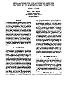
Figure 3.4: An illustration of the architecture of AlexNet deep convolutional neural network, showing the dimensions of each layer. The input layer is followed by 5 convolutional layers (Conv1-5), the output of the fifth convolutional layer is fed into two Fully-connected layers (FC6-7), then the output is a fully-connected 1000-way soft-max layer (FC8).

million labeled images, belonging to roughly 22,000 object categories. ILSRVC is an annual competition on a subset of ImageNet dataset in which it is required to classify images into 1000 object category, with roughly 1000 training images for each categories. Evaluation of results in ILSRVC are done using top-1 and top-5 error rates. Top-1 error rate is the fraction of images for which the correct label is not the predicted label, and top-5 error is the fraction of images for which the correct label is not in the top 5 classes which the method considers most probable. AlexNet achieved a significant improvement in classification results in ILSVRC 2012, with a top-5 error rate of 15.3%, while the second-best competitor achieved a top-5 error rate of 26.2%. AlexNet architecture, shown in figure 3.4, consists of an input layer that takes a 224x224 RGB image, followed by five convolutional layers (called Conv1-5), followed by two fullyconnected layers (called FC6 and FC7), and finally a fully-connected output layer which is fed to a 1000-way softmax (called FC8). The softmax maps the 1000 arbitrary values to 1000 probabilities in range [0,1] with sum 1, hence producing prediction probabilities across the 1000 object categories. Each convolutional layer convolves its input with a set of 3D kernels, and then applies point-wise non-linearity. The fully-connected layers are normal neural network layers, which also apply point-wise non-linearity. Each of the first, second and fifth convolutional layers are followed by max-pooling layers. The full network contains 650K neurons and 630M connections, which lead to 60M parameters to learn. The gap between number of connection and number of parameters is attributed to the weight sharing property in convolutional layers. More detailed information about the architecture is in the paper [18]. A common approach to apply non-linearity in neural networks is using sigmoid or tanh functions, which are considered saturating nonlinearities. AlexNet use Rectified Linear Unit (ReLU), defined as f (x) = max(0, x), to provide non-saturating nonlinearity. Using ReLUs nonlinearities results in training several times faster than using tanh non-linearity. In AlexNet, ReLUs are applied to the output of all convolutional and fully-connected layers. Similar to all CNNS, each convolutional layer in AlexNet acts as a feature extractor. As an example, figure 3.5 shows the learned kernels in the first convolutional layer (Conv1). Conv1 19

Figure 3.5: Kernels learned from AlexNet’s first convolutional layer. learns 96 kernels of size 11x11x3, which operate on the input RGB images. As appearing in the figure, these kernels are similar to a variety of edge filters. Subsequent convolutional layers learn kernels that recognize more complex structures, thus generating rich mid-level representations of the input images. Following the feature extracting convolutional layers, fully connected layers are used to perform feature reduction and classification on top of the extracted rich mid-level representations. One of the strengths of AlexNet is that it takes raw RGB images as its input; no feature extraction is needed prior to feeding the network. The only preprocessing step is calculating a mean image from the training set, and subtracting this mean image from each input image in training and testing. To handle images of variable resolutions, as in the case of ImageNet dataset, images are down-sampled to a resolution of 256x256. First, the image is scaled so that its shortest dimension is 256. Then a rectangular patch of size 256x256 is cropped from the center of the image. As explained next, this 256x256 image is used to generate the 224x224 input for AlexNet. Since the network has 60M parameters to learn, it is prune to overfitting the training data. To decrease the probability of overfitting, AlexNet uses two data augmentation techniques to increase the amount of training data. At training time, random patches of size 224x224 are extracted from the 256x256 images generated by down-sampling training images. They further increase the training set by generating horizontal reflections for each of the 224x224 patches. Consequently, the input layer of AlexNet is 224x224x3 as it takes these generated 224x224 RGB patches. Without this data augmentation approach, AlexNet suffers from significant overfitting. At test time, they generate ten 224x224 patches from each of the 256x256 test images, and average the prediction probabilities on the ten patches. These patches are generated by taking four 224x224 corner patches and one center patch, in addition to their horizontal reflections. The second technique used for data augmentation is altering the intensities of the RGB channels in training images. They perform Principal Components Analysis (PCA) [50] on RGB pixel values in the training set images. Then for each training image, they add to each RGB pixel random values proportional to the found principal components and their corresponding eigenvalues. This technique introduces variations in intensity and color of image’s illumination, forcing the model to learn object properties invariant to illumination changes. A successful method commonly used to reduce overfitting is combining predictions of multiple trained models. This method is hard to use in the case of deep learning as training one model takes several days. A method called dropout [51] was introduced to mimic this 20

models-combination technique while costing only double the training time. While processing each training sample, half the neurons in a layer are randomly disabled by setting their output to zero. The dropped out neurons do not contribute to this training iteration, practically forming a different network architecture with each training sample. As a result of using dropout, a hidden neuron cannot rely on other hidden neurons being present, this forces it to learn detecting features given a large variety of context modeled by its inputs, therefore, it learns robust features. At test time, dropout is not used and all neurons are enabled. To compensate for the fact that twice as many neurons are active, the network weights are set to half their trained values. In AlexNet, dropout is used in the first two fully-connected layers (FC6 and FC7), which as a result doubles the required training iterations to reach convergence.

3.1.3.4

Transferring learned AlexNet information to other domains

AlexNet is trained on a massive data set, ImageNet ILSVRC, which comprises 1.2 million training images across 1000 object categories. Due to the variety and size of the training data, AlexNet learns generic feature extractors, which generate rich mid-level representations. In order to train AlexNet on new data, massive amount of labeled data is needed, which is not always available. Multiple approaches were suggested in previous studies to adapt AlexNet’s learned rich mid-level representations to new domains, without losing the information learned from ImageNet. An interesting method to utilize the information captured by AlexNet is using the 4096dimensional activations at the last fully-connected hidden layer (FC7) as discriminative features. This method is used in AlexNet’s paper [18] to provide qualitative demonstration of AlexNet’s capabilities. Two images are considered similar if their corresponding 4096dimensional activation features have small Euclidean distance. They generated the 4096dimensional for some query images from the test set, and used the aforementioned method to retrieve similar training set images. This experiment resulted in retrieving images that are semantically similar to the query image, although they have significantly different visual properties. Although FC7 features provide discriminative features in many domains, this technique does not utilize training data from the target domain. Transferring learned information from source domain (ImageNet) to target domain could be performed through fine-tuning process, which requires much less data than training from scratch. Fine-tuning uses an already trained CNN as a base, and performs the following steps: 1. Replace the last layer (FC8) with a fully-connected output layer with N-way softmax, where N is the number of classes in the target domain. 2. Initialize the newly added output layer with random weights. Keep weights of other layers as trained in source domain. 3. Train the whole network using target data. Usually the learning rate of old layers are set to be lower than the newly added output layer. This is done to adapt network weights to new domain data, without losing the rich representation learned from source domain. 21

Figure 3.6: Representation of star-shaped structure of DPM, showing spring connections between parts (yellow boxes) and root (red box). Figure is from [52]. As detailed in the literature review, many recent studies applied fine-tuning to use AlexNet in other domain, which helped them reach state-of-the-art results.

3.1.4

Deformable Part Models (DPM)

Object detection is one of the integral tasks in computer vision; various research was done to tackle the challenge of detecting and localizing certain objects in images. One of the interesting lines of research is using part-based models to perform object detection. Partbased models represent an object using attributes of object parts and their geometric relations. These techniques are robust to object variability; they are capable of representing objects that possess various shapes and orientations. We use the state-of-the-art part-based technique introduced by Felzenszwalb et al. [27], called Deformable Part Models (DPM). Since surgical tools are seen from different angles in laparoscopic videos, and they change their shapes dramatically during usage, this motivates the choice of using part-based models for detecting surgical tools. DPM’s strength comes in three-folds; first, it represents an object using a mixture of part-based models, called components, which accommodates for the different viewpoints. Second, each part-based model is a multiscale star-shaped model, which captures nonrigid deformations in object shape. Finally, it uses a discriminative training procedure that accommodates for partially labeled data, and is robust to inaccuracies in the labels. Although we are only interested in detecting usage of surgical tools in video frames, DPM provides a powerful system that helps inferring reliable information about surgical tools’ existence in video frames. A DPM model consists of a root filter and a set of part filters, all based on Histograms of Oriented Gradients (HOG) features. The root filter represents the shape of the whole object, while part filters represent discriminative regions in the object. Each part has an anchor position, relative to the root, where it is expected to be found. Geometric alignment of parts relative to the root is subject to a star-shaped structure, where each part have a spring-like connection to root’s center; i.e. each part is allowed to move far or near to the root, but with a penalty. The penalty of a part deviating from its anchor position is called deformation cost. Figure 3.6 illustrates the star-structure of DPM model. It is worth noting that parts in DPM does not have semantic meanings, their positions are set during the training procedure according to variability in object shape, hence they do not correspond to physical parts of the object. 22

Part filters in DPM capture HOG features from a resolution twice the resolution where root filter capture HOG features. As a result, the root filter describes coarse object information, such as its outline and basic shape, while part filters describe fine details in the object. Incorporating coarse and fine information leads to higher accuracy in object detection and localization. To demonstrate DPM models, we show in figure 3.7 the trained DPM model for one of cholecystectomy surgical tools; the hook. The figure shows that each component captures different viewpoint of the hook tool. By examining part locations, you can confirm the fact that DPM parts are not associated with the object’s physical parts. Moreover, we show in figure 3.8 a sample detection for hook tool using this model, and the corresponding part filters. Training DPM object detectors is done using a discriminative procedure called Latent SVM (LSVM), this procedure requires only bounding boxes, labeled around training instances, to learn DPM models. Since the locations of parts in objects are not labeled, they are considered latent variables during training. LSVM is designed to deduce latent variables, and use them in optimizing the trained models. One advantage of using LSVM is that labeling bounding boxes around objects of interest is faster and easier than labeling all object’s parts. Furthermore, this allows the training framework to learn parts’ shapes and locations automatically, which eliminates the need for a manual definition of object’s parts, which could be suboptimal and results in inferior training. One could expect that, during training, root locations should be taken from the ground truth bounding boxes. However, in training DPM, root locations are treated as latent variables with a constraint that they have high overlap with the ground truth bounding boxes. This approach accommodates for noisy labeling of bounding boxes, which commonly occurs due to human labeling errors. This approach produces strong object models without the need to correct noisy labels. We refer readers interested in more details about DPM training to [27]. In order to detect a certain object, DPM utilizes a sliding window approach across different scales of the test image. A window of the same size as model’s root is slided across the image, each location is considered a hypothesis for an object’s root location. For each root hypothesis, there exists large number of possible placements of parts relative to the root. DPM scores an object hypothesis, consisting of hypotheses of root and parts positions in the test image, using the equation: score = Froot · φ(proot ) +

n X

Fi · φ(pi ) −

i=1

n X

di · (dxi , dyi , dxi2 , dy2i ) + b

(3.16)

i=1

where Froot is the root filter, Fi is the i-th part filter, proot is the hypothesized root location, pi is the hypothesized location of the i-th part, n is the number of parts, φ(p) is the HOG features extracted at location p in the test image, di is the deformation parameters for the i-th part, dxi and dyi are the displacement of the i-th part from its anchor position, operator · is the dot product, and b is the bias term. Note that Froot , Fi , di , and n are parameters of the trained model, while other parameters are derived from the scored hypothesis. Typically, a DPM model is associated with a threshold, if the score of an object hypothesis is less than the threshold, this detection is discarded, else an object instance was found.

23

(a)

(b)

(c)

Figure 3.7: DPM model for hook tool. Each row shows the figures for one component. Each component is defined by (a) a root filter, (b) eight part filters at double the resolution, and (c) parts deformation cost. White color represents the highest value, and black color represents the least value.

(a)

(b)

Figure 3.8: Sample hook detection (a), and its corresponding part filters (b). 24

The first and second terms in equation 3.16 represent the scores of the root and part filters, while the third term, the deformation cost, enforces spatial constraints on part locations. Deformation parameter di defines how part deformation from its anchor position is penalized. The resulting deformation cost is a quadratic function of part displacement from its anchor position. As an example, if di is (0,0,1,1), the deformation cost would be the square of the distance between part location and its anchor position. Testing all possible part locations, for a certain root hypothesis, is an expensive procedure. Felzenszwalb et al. [27] devised a fast dynamic programming algorithm, based on distance transform, to find the placement of parts that results in the highest score for a certain root position. This makes testing all possible hypotheses more feasible than the exhaustive approach. Since DPM represents different viewpoints of the object using a mixture of components, the aforementioned sliding window approach is repeated to generate object detections for each component in the DPM model. The bias term in equation 3.16 makes detection scores comparable across DPM components. Since detection is done using a sliding window at different scales, DPM usually results in multiple overlapping detections for the same object instance. To solve this problem, Felzenszwalb et al. use the non-maximum suppression procedure. If two detections have more than 50% overlap, the detection with higher score is taken, and the lower scoring detection is deleted.

3.2

Features

In this section, we first introduce the handcrafted features used as baseline in our experiments. Afterwards, we introduce the features we use in our proposed pipeline, which are a mixture of mid- and high- level features. Mid-level features are complex and rich features that represent the underlying semantic information, but does not provide full semantic information. As for high-level features, they are features that give independent information that could be used directly in other tasks. We discuss in this section the specific mid- and high- level features we use, and we explain the method we employ for extracting these features.

3.2.1

Baseline features

For establishing our baseline for the surgical workflow detection task, we chose the handcrafted features used by Twinanda et al. [53] as the features to train the one-vs-all SVMs. We chose these features as our baseline features for two main reasons; a) they consist of low-level features similar to those used by Blum et al. [11] with an addition of SIFT [54] descriptors, b) Twinanda et al. used these features for classification of laparoscopic videos, which is a task similar to our problem. Twinanda et al. use three categories of features, which are: 25

Feature

Dimensionality

Number of Words

RGB

48

300

HS

72

300

SIFT

128

1000

HOG

288

1000

Table 3.1: Twinanda et al. [53] features’ dimensionality, and number of words for BoVW models.

Color Histograms. Inspired by the color differences between human organs and surgical tools, this work extracts histograms of Hue-Saturation (HS) from the HSV color space and extracts histograms of Red-Green-Blue (RGB) colors. It uses 36 bins for each of the two HS histograms, and it uses 16 bin for each of the three RGB histograms. SIFT. Since the position and scale of inner body organs and surgical tools vary tremendously in laparoscopic videos, this work uses SIFT key point detectors and SIFT descriptors [54] to benefit from SIFT’s scale and rotation invariance. HOG. To capture possible information in the video frames from a global perspective, this work uses Histograms of Oriented Gradients (HOG) [55]. Twinanda et al. use bag-of-visual-words (BoVW) model [56] on top of the aforementioned features. We show in Table 3.1 the features’ dimensions, and the number of words used in their corresponding BoVW models.

3.2.2

Mid-level features: CNN activations

The first type of features we propose to use is mid-level features extracted using a finetuned AlexNet Convolutional Neural Network. We employ finetuning in order to transfer AlexNet’s learned information from ImageNet domain to cholecystectomy phase recognition domain. Following the finetuning process, we replace the last layer in AlexNet with a fullyconnected output layer with N p -way softmax (called FC8 phase), which infers recognition probabilities for the N p possible phases. We illustrate the resulting architecture in figure 3.9. We randomly initialize the added layer’s weights, and follow the finetuning procedure described in section refsec:finetune. To extract the mid-level CNN features, we follow Girshick et al. [23] in using the last hidden layer’s activations (FC7) as our features. First, we resize the cholecystectomy video frame to 256x256 pixels. Next, we crop a patch from the resized frame’s center, with dimensions equal to the fine-tuned CNN’s input layer’s dimensions, i.e. 224x224. Afterwards, we subtract ImageNet mean image from the cropped path, and feed the resulting image into the fine-tuned CNN. Finally, we extract the 4096-D output activations from FC7 to be our features. This results in mid-level features φCNN ∈ R4096 . 26

Figure 3.9: The CNN architecture we use for extracting mid-level features, based on AlexNet architecture. We replace the last layer in AlexNet (FC8) with a fully connected layer with 7-way softmax (FC8 phase), and then fine-tune the network on our data.

Figure 3.10: Representation of tools’ usage in two sample cholecystectomy procedures. Vertical dashed lines represent surgical phases’ boundaries. Horizontal bars represent usage of corresponding tool across time. It is clear that some tools’ usage information could be used to identify some surgical phases.

3.2.3

High-level features: Tools presence probabilities

By examining surgical tools’ usage in cholecystectomy procedures, as in figure 3.10, we can evaluate the relationship between used tools and surgical phases. Some surgical tools, such as grasper, are used throughout the surgery. Yet, other tools are mostly used in specific phases, such as clipper and scissors that are usually used in the clipping and cutting phase. This observation emphasizes the importance of utilizing tools’ usage as a discriminative feature for surgical phase recognition. Furthermore, as discussed in the literature review, previous work used rich information about tools’ usage to do the surgical workflow detection task. Tools’ usage information is provided either manually by an expert, or automatically such as using radio frequency identification (RFID). Since we aim at using only visual information in our method, we propose to train DPM object detectors to detect the presence of surgical tools, and use the output of these detectors as high-level features. For each of the Nt surgical tools used in cholecystectomy surgical procedure, we train a DPM detector to detect the presence of this tool. To be used as features, we use the Nt trained 27

(a)

(b)

(c)

Figure 3.11: Sample DPM detections for (a) grasper, (b) hook , and (c) clipper surgical tools. Root filter detection is shown as a red box, and part filter detections are blue boxes.

DPM detectors to get the probability of tools’ presence in each video frame. Each DPM detector results in multiple tool hypotheses, we choose the highest hypothesis confidence to be the confidence of corresponding tool’s existence in this video frame. Thus we get high-level features φDPM ∈ RNt , which represent the probability of presence for the Nt surgical tools. We show in figure 3.11 sample detections for some of the surgical tool in cholecystectomy procedure.

3.3

Full pipeline

In our proposed method, we use the 4096-dimensional activation values from FC7 from our fine-tuned CNN as the mid-level features φCNN ∈ R4096 . The second type of features we use is the high-level features φDPM ∈ RNt , which are generated using the trained DPM tool detectors, where Nt is the number of surgical tools used in cholecystectomy surgical procedure. We incorporate the information from both types of features through two different approaches. In both approaches, we calculate V which is utilized to generate the observations for the used HHMM. The first proposed pipeline is represented in figure 3.12. We calculate V ∈ RN p , where N p is the number of surgical phases, as follows: 28

Algorithm 1 PhaseNet + DPM 1: Generate DPM probabilities φDPM 2: Generate CNN features φCNN 3: Concatenate φCNN and φDPM to get φboth 4: for each phase k do 5: Use concatenated features φboth to calculate SVM score vk 6: Concatenate the SVM scores v1 to vN p to get V The second pipeline is represented in figure 3.13. We calculate V ∈ RN p +Nt , where Nt is the number of detected surgical tools, as follows:

Algorithm 2 PhaseNet + direct DPM 1: Generate CNN features φCNN 2: for each phase k do 3: Use the features φCNN to calculate SVM score vCNNk 4: Concatenate the SVM scores vCNN1 to vCNNN p to get vCNN 5: Generate DPM probabilities φDPM 6: Concatenate VCNN and φDPM to get V The difference between both pipelines is in the way we incorporate DPM features φDPM in our pipeline; The first pipeline concatenates DPM and CNN features, then feeds both of them to the one-vs-all SVMs as shown in figure 3.12, then the outputs of the SVMs are fed to the HHMM to generate its observations. The second pipeline considers DPM features φDPM to be comparable with the confidence scores VCNN resulting from the one-vs-all SVMs, consequently concatenating φDPM with VCNN , then feed the result to the HHMM to generate its observations, as shown in figure 3.13. We chose to use the second pipeline in our proposed method. This choice is motivated by the fact that this approach considers the high-level nature of the DPM features in incorporating it with the CNN features. Moreover, the number of CNN features is much larger than the DPM features, which leads to a bias in the first approach since they are concatenated without any processing. However, the first pipeline is useful for comparing our features with the other types of features.

29

Figure 3.12: Concatenating DPM confidences with CNN features, then using them as input to the one-vs-all SVMs.

Figure 3.13: Concatenating DPM confidences with outputs of the one-vs-all SVMs.

30

Chapter 4: Experiments and Results 4.1

Cholec80 Dataset

We performed our experiments on the Cholec80 dataset [7], which was recorded at the University Hospital of Strasbourg and labeled at ICube Laboratory, Strasbourg University. This dataset consists of 80 videos of cholecystectomy procedures performed by 13 surgeons. We split the dataset into two equal sets; 40 videos for training our feature extractors, and use the remaining 40 videos for evaluating the performance of our proposed features. Cholec80 dataset was recorded at 25 fps, but we use the first frame at each second for our experiments. We do this downsampling of the videos to 1 fps to reduce the redundancy in training and evaluation data, in addition to reducing the computational overhead of the experiments. The dataset contains two types of annotations; (a) phase annotations, and (b) surgical tool annotations. We present details about these annotations in the following subsections.

4.1.1

Phase annotations

With the guidance of a senior surgeon in Strasbourg University Hospital, we defined seven surgical phases for the cholecystectomy procedure. The defined phases are consecutive; a phase starts with the end of another phase. We define the phases as follows: • Preparation (P1): Starts with inserting the laparoscopic camera into the patient’s abdomen and ends with the first usage of a cutting tool. • Calot’s triangle dissection (P2): Starts with the surgeon removing the fat in Calot’s triangle and ends with inserting the clipper tool. • Clipping and cutting (P3): Starts with the clipper tool inserted into the patient’s abdomen and ends with both the cystic duct and the cystic artery clipped and cut. • Gallbladder dissection (P4): Starts with the gallbladder disconnected from the liver and ends with the gallbladder completely detached from the liver bed. • Gallbladder packaging (P5): Comprises putting the detached gallbladder into a specimen bag. • Cleaning and coagulation (P6): During this phase the surgeon stops any hemorrhaging inside the abdomen and clean the traces of blood or bile leaked during the procedure. • Gallbladder retraction (P7): Comprises retracting the specimen bag, with the gallbladder inside it, from one of the trocars. To further understand these phases, we refer you to the details about cholecystectomy procedure in section 1.1. Figure 4.1 shows video screenshots representing each phase. We defined these seven phases according to the main surgical events in cholecystectomy procedure, consequently the resulted phases’ duration vary tremendously. We show the mean and standard deviation of phases’ duration in Table 4.1. Phases occur in the same order as 31

Preparation (P1)

Calot’s triangle dissection (P2)

Clipping and cutting (P3)

Gallbladder dissection (P4)

Gallbladder packaging (P5)

Cleaning and coagulation (P6)

Gallbladder retraction (P7)

Figure 4.1: Video screenshots representing each of the seven phases labeled in Cholec80 dataset.

32

ID

Phase

Duration (s)

P1 P2 P3 P4 P5 P6 P7

Preparation Calot triangle dissection Clipping and cutting Gallbladder dissection Gallbladder packaging Cleaning and coagulation Gallbladder retraction

125±95 954±538 168±152 857±551 98±53 178±166 83±56

Table 4.1: List of phases in the Cholec80 dataset, including the mean ± std of phases’ durations in seconds across all videos. Table from [7]. defined, except for some cases where P6 occur before P5 or after P7. All phases are labeled in each video, with an exception of some videos that do not go through P6 (cleaning and coagulation phase). It is worth noting that phases boundaries are artificially defined; in reality there exists some transitional periods between phases, with no surgical activities, which do not belong to any of the defined phases.

4.1.2

Surgical tool annotations

Surgeons use seven surgical tools in cholecystectomy procedure, which are: • • • •

Grasper: Used for holding and handling organs and tissues throughout the surgery. Hook: Used for removing fat and dissecting tissues. Clipper: Used for putting clips on ducts and arteries to stop fluids flow. Scissors: Used for cutting ducts and arteries. Sometimes it is used for dissecting tissues. • Biploar: Used for stopping any bleeding that occur throughout the surgery. • Irrigator: It has two modes, in the first mode it releases water inside the abdomen. In the second mode it is used to suck fluids. Both modes are used for cleaning. • Specimen bag: After the gallbladder is completely detached, it is put in this bag to be retracted to outside the body. Figure 4.2 shows these seven tools, and samples from their usage in cholecystectomy procedures. In each video frame across the Cholec80 dataset, we labeled the presence of each of the seven tools. These annotations are binary annotations that only describe the visibility of these tools in each video frame. We consider a tool to be visible if at least half of its tip is visible in the frame. In some cases, we can see the shaft of the tool but the tip is not visible, we consider the tool not visible in this case. We call this the tool presence annotations. The second type of annotations labeled for surgical tools is the bounding box annotations. In some videos from the Cholec80 dataset, we labeled a tight box on the surgical tool’s tip. These bounding boxes are needed for training DPM tool detectors. A bounding box is 33

Grasper

Hook

Clipper

Scissors

Biploar

Irrigator

Specimen bag

Figure 4.2: The seven surgical tools used in cholecystectomy surgical procedures that comprise the Cholec80 dataset. Top row are the seven tools, and bottom row are samples of their usage in Cholec80 videos.

Figure 4.3: This figure shows the split of Cholec80 dataset into fine-tuning and evaluation subsets. It illustrates that the 10 DPM training videos are part of the fine-tuning subset. labeled in the cases where the tool is visible, following the same criteria defined for tool presence annotations. This implies that whenever a bounding box is present, the tool presence label is set to 1. On the contrary, in some frames the tool presence label is 1, but there are no bounding boxes for this tool. This happens when the tool is far from the camera or is blurry. We decided to avoid labeling bounding boxes for these cases as they will be difficult to localize by the trained tool detectors. These cases will confuse the detectors and will not have any added value in the training process. We labeled the bounding boxes for the tools in 10 videos, except for the grasper and the hook where we found that 3 videos resulted in sufficient number of instances.

4.2

Experimental setup

We split the Cholec80 dataset into two equal subsets, each containing 40 videos. The first subset is used for fine-tuning the CNN. Additionally, we use 10 videos from the finetuning for training the DPM tool detectors. These are the 10 videos that have bounding box annotations. The second 40-videos subset is used for evaluating the proposed features. Figure 4.3 illustrates these splits. We use Caffe framework [21] to fine-tune the CNN and extract our mid-level features. Our base CNN model is the ”bvlc reference caffenet” model (called CaffeNet) provided with Caffe framework [57]. It is based on the AlexNet architecture [18] with minor variations in architecture and training. There are three main differences between CaffeNet and AlexNet; 34

Parameter

Value

Number of iterations

310 K

Batch size

256

Initial learning rate

0.01

Momentum

0.9

Weight Decay

0.0005

Step size

100 K

Gamma

0.1

(a) Pre-training parameters.

Parameter

Value

Number of iterations

50 K

Batch size

50

Pre-trained layers learning rate

0.001

New layers learning rate

0.01

Momentum

0.9

Weight Decay

0.0005

Step size

20 K

Gamma

0.1

(b) Finetuning parameters.

Table 4.2: Values for training parameters used in a) pre-training our CNN on ImageNet data, and b) fine-tuning the CNN on our data.

First, CaffeNet is not trained with the data augmentation method used by AlexNet. Second, max pooling is done in CaffeNet before local response normalization, while in AlexNet it is the opposite. Third, there are minor changes in layers dimensions between AlexNet and CaffeNet, e.g. input layer in CaffeNet is 227x227, while in AlexNet it is 224x224. CaffeNet is pre-trained using ImageNet Large Scale Visual Recognition Challenge 2012 dataset (ILSVRC 2012) [19]. In pre-training CaffeNet, the weights of the network layers are initialized using a zeromean Gaussian distribution with standard deviation 0.01, except for FC6 and FC7 where the standard deviation is 0.005. As for fine-tuning, the weights of the added layer (FC8 phase) are initialized similarly with standard deviation 0.01, while the weights of the other layers are taken from the pre-trained models. We list in table 4.2 the rest of the parameters used in pre-training CaffeNet on ImageNet data, and in fine-tuning the model on our data. For tool detection, we train the DPM models using the code provided by Girshick et al. [58]. We set the number of components to be 3, and use the other parameters as set by the authors. As specified in [59], the trained models contain 8 parts, where each part consists of 35

6x6 HOG cells (48x48 pixels). We train a separate DPM model for each of the 7 tools. We use bounding box annotations as the positive samples. Negative samples are extracted from the frames where the tool is not visible; i.e. tool presence annotation is 0. We do not use other tools’ bounding boxes as negative samples, which might improve the trained models. However, they are implicitly included as they appear in the negative frames. To evaluate the proposed features, we perform 4-folds cross-validation on the 40 evaluation videos. Three folds are used to train the one-vs-all SVMs and the HHMM, while the 4th fold is used for testing the whole pipeline. Since our proposed pipeline contains stochastic modules, such as the SGD training algorithm, we repeat each evaluation experiment five times and report the average of the five runs. We use VLFeat library [60] for training and using SVMs. In the cases where we use kernel SVMs, we use VLFeat to approximate kernel maps as proposed in [36]. As for the HHMM, we used the code from [32] with minor modifications.

4.3

Evaluation metrics

In order to evaluate phase recognition results, we use the following metrics: • Average Precision (AP): Calculated as the average of recognition precision for all phases, where recognition precision for each phase is: Number of frames successfully detected as belonging to this phase Number of frames detected as belonging to this phase • Average Recall : Calculated as the average of recognition recall for all phases, where recognition recall for each phase is: Number of frames successfully detected as belonging to this phase Number of frames in ground truth that belong to this phase • Accuracy : Calculated as: Number of frames successfully recognized Total number of frames As for evaluating tool detection, we follow the PASCAL Visual Object Classes (VOC) Challenge [61] in using precision-recall curve and average precision (AP), however, we define precision and recall differently. Since we are not interested in object localization, tool detection is defined per frame, not per tool instance. A tool is considered successfully detected if its detection confidence in the frame is higher than a defined threshold. The precision-recall curve is generated by calculating detection precision and recall at all possible threshold values. Average Precision (AP) is a replacement of the Area Under Curve (AUC) measure, which provides a more sensitive metric to highlight differences between methods. To obtain high AP, an object detector should provide precise results at different recall levels. This penalizes 36

detectors that provide results of high precision for only a subset of testing examples. In PASCAL VOC Challenge [61], AP is defined as: AP =

1 11

X

pinterp (r)

(4.1)

r ∈ {0,0.1,...,1}

where pinterp (r) is the interpolated precision for a certain recall level, which is calculated as the maximum precision achieved with recall higher than r: pinterp (r) = max p(˜r) r˜ : r˜ ≥ r

(4.2)

where p(˜r) is the precision at recall r˜. Interpolation is used to reduce the effect of ”wiggles” in the precision-recall curve.

4.4

Experimental results

We compare our proposed features to the following features: • GT binary tool: Using manual annotations for tool presence as features. This provides a simulation for using external tool information. • Handcrafted: The baseline features presented in section 3.2.1. • Handcrafted + CCA: Similar to the approach suggested by [11], we employ tool presence annotations to perform feature selection on handcrafted features through canonical correlation analysis (CCA). • AlexNet: Output activations from FC7 in the CNN after pre-training on imagenet. • PhaseNet: Output activations from FC7 in AlexNet after fine-tuning on Cholec80 dataset. • PhaseNet + DPM: Concatenation of the aforementioned PhaseNet features with DPM confidences, as explained in figure 3.12. Each of these features are used as input to the pipeline in figure 3.1. Additionally, we compare the phase recognition results using the above features to our method using the pipeline presented in figure 3.13. Comparison of the different features against our proposed method are shown in table 4.3. In all these experiments, we model HHMM observations using a mixture of 5 Gaussians, except for the case of GT binary tool features, where we use 1 Gaussian. In the handcrafted features experiment, we use histogram intersection kernel SVMs, while in the rest of the experiments we use linear SVMs. Table 4.3 shows that replacing handcrafted features with AlexNet features improves the accuracy by 15 points in offline mode, and 29 points in online mode. This major improvement is achieved by the CNN trained on ImageNet data, which proves the strength of the learned network and its capability to represent general structures in different domains. Further improvement is achieved by using PhaseNet; the CNN fine-tuned on Cholec80 dataset. It increases accuracy by 13 points in offline mode, and 11 points in online mode. Using both CNN and DPM features, following the pipeline in figure 3.13, results in minor improvement 37

Feature

Overall-Offline (%) Avg. Precision

Avg. Recall

Accuracy

GT binary tool

68.4±24.1

75.7±13.6

69.2±8.0

Handcrafted

40.3±20.4

40.0±17.8

36.7±7.8

Handcrafted + CCA

54.6±23.8

57.2±21.2

61.3±8.3

AlexNet

70.9±12.0

73.3±16.7

76.2±6.3

PhaseNet

82.5±9.8

86.6±4.5

89.1±5.4

PhaseNet + DPM

82.65±0.42

87.61±3.99

89.03±5.51

PhaseNet + direct DPM

83.70±10.50

88.25±4.90

90.47±3.46

(a) Results in offline mode.

Feature

Overall-Online (%) Avg. Precision

Avg. Recall

Accuracy

GT binary tool

54.5±32.3

60.2±23.8

47.5±2.6

Handcrafted

31.7±20.2

38.4±19.2

32.6±6.4

Handcrafted + CCA

39.4±31.0

41.5±21.6

38.2±5.1

AlexNet

60.3±21.2

65.9±16.0

67.2±5.3

PhaseNet

71.3±15.6

76.6±16.6

78.8±4.7

PhaseNet + DPM

72.3±15.6

78.2±8.1

79.9±5.4

PhaseNet + direct DPM

73.3±17.4

78.9±6.3

80.6±5.1

(b) Results in online mode.

Table 4.3: Comparison of phase recognition results (mean ± std) on Cholec80 dataset in: (a) offline mode, and (b) online mode. The best result for each evaluation metric is written in bold. Some of the presented results are from [7]. Results from our proposed method (figure 3.13) are presented in the last row.

38

P1

P2

P3

P4

P5

P6

P7

Prec.

89.6±10.7

98.1±1.2

72.7±13.7

94.6±3.7

71.5±7.1

80.4±8.2

79.0±11.6

Rec.

92.4±4.3

90.3±7.8

86.5±10.3

93.6±3.0

90.8±2.9

80.1±10.4

84.1±10.2

(a) Per phase results in offline mode.

P1

P2

P3

P4

P5

P6

P7

Prec.

91.5±9.2

97.0±1.1

70.4±13.2

81.3±6.8

50.4±8.7

65.5±9.2

57.2±17.6

Rec.

80.4±11.0

78.4±9.9

70.0±11.8

86.3±4.1

80.1±3.7

71.3±12.0

85.7±7.9

(b) Per phase results in online mode.

Table 4.4: Precision and recall of phase recognition for each phase on Cholec80 using the proposed features (PhaseNet + direct DPM). in both modes. This minor improvement suggests that the fine-tuned CNN already captured much information about the used tools. For all the compared features, the performance in offline mode is better than in online mode. This is the result of the different nature of the two modes. In online mode, the video is processed frame by frame, only given the knowledge of the previous frames. As a result, the HHMM corrects phase predictions along the video as soon as it gets information from new frames. On the contrary, in offline mode the video is processed as a whole. This gives HHMM enough information to provide a more accurate prediction for the whole video. To further examine the performance of our proposed method, we provide detailed perphase results in table 4.4. In offline mode, all the phases yield high numbers in both precision and recall. In online mode there is a drop in performance in the last three phases, this is attributed to the fact that the order of these phases interchange in some training and testing videos. This result in multiple transition options for these phases, which increases the difficulty of the HHMM decision. This problem does not occur in offline mode, since the Viterbi path algorithm is capable of inferring the correct order of these phases given the knowledge of the whole video. To evaluate the trained surgical tool detectors separate from the whole pipeline, we show in figure 4.4 the precision-recall curves of the trained DPM detectors, which illustrate the performance of each of the seven tool detectors. Additionally, we show in table 4.5 the average precision evaluated on the 40-videos evaluation subset. All tool detectors yield high average precision, except for the scissors. The low performance of scissors’ detector could be attributed to its low number of training instances. Furthermore, the shape of the scissors is similar to the grasper, which is more abundant in the dataset. Since the DPM detector only captures shape information, it fails to model the scissors effectively, resulting in a confusion between the grasper and the scissors. To demonstrate the added value of using HHMM in our method, we compare in table 4.6 the results of our method without using HHMM versus the full method. To provide a fair comparison, we present results of using the method proposed in figure 3.12 as it utilizes 39

Grasper

Hook

Clipper

Scissors

Biploar

Irrigator

Specimen bag

Figure 4.4: Precision-Recall curves for surgical tool detection using DPM.

40

Tool

Avg. precision (%)

Bipolar

60.6

Clipper

68.4

Grasper

82.3

Hook

93.4

Irrigator

40.5

Scissors

23.4

Specimen bag

40.0

Mean

58.4

Table 4.5: Average precision (AP) for DPM tool detectors, computed on the 40 videos forming the evaluation dataset of Cholec80. Results from [7].

both mid- and high- level features in inferring phase prediction using one-vs-all SVMs, thus the HHMM refines initial predictions done by the SVMs without using any additional information. As explained in section 3.1.2, the predictions performed by the one-vs-all SVMs is the same in both online and offline modes, the difference between online and offline modes is in the procedure used for inferring the phases using HHMM. Accordingly, table 4.6 compares the results of our method without using HHMM versus using HHMM in both online and offline modes. It is clear from table 4.6 that adding HHMM refines the inferred phase detection in both online and offline modes. In online mode, adding HHMM to our pipeline achieves 5 points increase in average precision and 15 points increase in average recall. Further improvement is achieved in offline mode with 15 points increase in average precision, and 24 points increase in average recall. We highlight in table 4.6 the results where using HHMM decreases the prediction precision, which is the case for P3 and P5. Nevertheless, the recall of these phases is improved by using HHMM. This is attributed to the fact that these phases have short duration, thus they does not possess enough discriminative information. The HHMM confuses these phases with the other phases, yielding a dramatic drop in precision.

4.5

Medical applications

In this section, we provide examples of medical applications for our proposed method. First, we discuss using surgical workflow detection for indexing cholecystectomy procedures, providing experimental results using our method. Second, we demonstrate that the tool detectors we trained could be used for providing notifications to supervising surgeons when certain surgical tools are used. 41

P1

P2

P3

P4

P5

P6

P7

Average

No HHMM

57.7±9

77.1±5

71.3±14

76.2±5

72.7±12

61.1±6

54.3±11

67.2±9

Online mode

87.2±8

95.1±3

63.2±15

81.4±7

54.8±11

66.1±11

58.0±17

72.3±16

Offline mode

86.0±10

95.6±4

68.7±20

95.4±3

72.7±6

81.4±8

78.7±13

82.7±10

(a) Comparison of per phase percision.

P1

P2

P3

P4

P5

P6

P7

Average

No HHMM

48.7±5

78.5±7

55.1±3

77.9±8

68.3±4

61.5±8

54.0±4

63.4±12

Online mode

79.5±12

78.9±10

64.8±14

84.8±5

80.6±4

70.4±16

88.3±9

78.2±8

Offline mode

92.1±3

88.8±11

85.0±8

91.2±5

89.9±4

80.9±10

85.5±10

87.6±4

(b) Comparison of per phase recall.

Table 4.6: Comparison of precision and recall for each phase on Cholec80 using the method in figure 3.12. First row in each table is the results without using HHMM, second row is using HHMM to refine results in online mode, and the third row is using HHMM to refine results in offline mode. We highlight in magenta the results where using HHMM decreases the precision.

4.5.1

Surgery indexing

Recorded cholecystectomy videos is usually used for training purposes, for documenting of the procedure, and for evaluating surgeons’ skills. One application of surgical workflow detection is indexing the surgical phases in a dataset of cholecystectomy videos. This indexing help in fast access of specific parts of the surgery, which save time and effort for the aforementioned applications. The task of surgery indexing is done after the surgery ends, which mean it is an offline mode application. In Table 4.7, we provide the results of Surgery indexing on the 40 test videos. Our method perform indexing with an error less than 30 seconds for 79% of the phases, and only 7.3% of the phases are indexed with an error more than 2 minutes. It is worth noting that these results are evaluated against the annotated phase boundaries, which are strict boundaries, while in practice there are idle period between phases that do not belong to any of the adjacent phases. As for this, an error less than 2 minutes yields the indexing to be correct in many cases. Since cholecystectomy procedures are in average more than 40 minutes long, correcting an error less than 2 minutes is a task faster and easier than indexing phases manually from scratch.

4.5.2

Clipper usage notification

One byproduct of our method is the trained tool detectors. These tool detectors could be used to provide notifications when certain surgical tools are used. The usage of some surgical tools provides interesting information about the surgery status, and could give an indication for upcoming complications. When a junior surgeon is performing the surgery, the tool detectors 42

Tolerance (s)

Phase P1

P2

P3

P4

P5

P6

P7