World Journal of Engineering and Technology, 2015, 3, 1-14 Published Online February 2015 in SciRes. http://www.scirp.org/journal/wjet http://dx.doi.org/10.4236/wjet.2015.31001
Using Neural Networks for Simulating and Predicting Core-End Temperatures in Electrical Generators: Power Uprate Application Carlos J. Gavilán Moreno Cofrentes Nuclear Power Plant, Iberdrola Generación Nuclear, Valencia, Spain Email:
[email protected] Received 13 January 2015; accepted 30 January 2015; published 3 February 2015 Copyright © 2015 by author and Scientific Research Publishing Inc. This work is licensed under the Creative Commons Attribution International License (CC BY). http://creativecommons.org/licenses/by/4.0/
Abstract Power uprates pose a threat to electrical generators due to possible parasite effects that can develop potential failure sources with catastrophic consequences in most cases. In that sense, it is important to pay close attention to overheating, which results from excessive system losses and cooling system inefficiency. The end region of a stator is the most sensitive part to overheating. The calculation of magnetic fields, the evaluation of eddy-current losses and the determination of loss-derived temperature increases, are challenging problems requiring the use of simulation methods. The most usual methodology is the finite element method, or linear regression. In order to address this methodology, a calculation method was developed to determine temperature increases in the last stator package. The mathematical model developed was based on an artificial intelligence technique, more specifically neural networks. The model was successfully applied to estimate temperatures associated to 108% power and used to extrapolate temperature values for a power uprate to 113.48%. This last scenario was also useful to test extrapolation accuracy. The method is applied to determine core-end temperature when power is uprated to 117.78%. At that point, the temperature value will be compared to with the values obtained using finite elements method and multivariate regression.
Keywords Neural Network, Error, Temperature, Core-End, Generator, Power Uprate
How to cite this paper: Gavilán Moreno, C.J. (2015) Using Neural Networks for Simulating and Predicting Core-End Temperatures in Electrical Generators: Power Uprate Application. World Journal of Engineering and Technology, 3, 1-14. http://dx.doi.org/10.4236/wjet.2015.31001
C. J. Gavilán Moreno
1. Introduction
In the power generation industry, there is a question with no consistent answer over time: should we invest in new generation assets and increase installed power? Or on the contrary, should we improve existing installations to increase their performance and therefore their power output as well? In economic scenarios such as the current one, in which power demand is stagnated and the expansion policies of most Western Europe utilities are a thing of the past, the question answered is the second one, relating to increased performance and power output of existing generation assets. By choosing the second option, investment is minimized and production unit costs optimized because, although actual production expenditure remains stable, energy generation increases. For all these reasons, many authors develop solutions based on power uprates or comprehensive performance enhancements [1]. The solution presented in this paper involves a power uprate applied to a synchronous generator, which considering that voltage is constant and increased intensity through stator coils. Without getting into the peculiarities of steam generation process limitations or combustion improvements, this type of solutions has a common bottleneck: the thermal capacity and margin of generator winding insulation. In terms of power uprate, these essential parameters are constraining because an increase of associated intensity results in higher generator conductor temperature, especially in the critical area known as end-core. That is the reason why it is vital to determine expected temperatures in these generator areas beforehand, as actual temperature values will condition the feasibility of power uprate and additional power. In other words, this determination will ultimately impact power uprate viability. After determining end-core temperature as a limiting parameter [2], it is time to perform calculations and extrapolations aimed at verifying if final extrapolated or calculated temperature is in fact below the acceptance criterion, which in this case will be the type B insulation limit (130˚C) [3]-[7]. Currently, there are two types of techniques to estimate end-core temperature: the finite element method (FEM) [8] and the regression estimation method [9]. The first method (FEM) is numerical, complex, more precise, resource intensive and requires an accurate internal generator geometry knowledge, which means that it is usually limited to OEMs or costly reverse engineering processes. Mathematically speaking, the second method is simpler and more accessible, but it renders more inaccurate results since the simulated process is significantly non-linear. The method proposed here is based on artificial neural networks because of their predictability, universal prediction, reality-adapted results, accessibility and easy implementation. The main challenge of this method is the need to have operational data from the machine under analysis so as to learn and create a reliable database from which to extrapolate power uprate results. Out of all neural networks, Feedforward architecture is chosen as it adapts to the purpose of adjusting and extrapolating. Using the abovementioned neural network requires a training process based on actual machine conditions and data, which means that it is necessary to have information on known operating states. Once the network simulates end-core temperatures with a minimum error under known conditions, it is time to extrapolate temperature values under power uprate conditions. In this case, there are available data for generator and end-core temperatures for an initial rated generator power of up to 108.57%. These data will be used to train the network and extrapolate end-core temperature values for power levels of up to 113.48%. Once this power is reached, the accuracy of the first extrapolation value will be checked. If extrapolation is accurate, the network will be rendered adequate and data will be gathered for a 113.48% power level which, together with available 108.57% power values, will be used to train the network and extrapolate data for a power level of 117.78%, which is what the licensee actually wants. The extrapolated value will be compared to the results obtained using the abovementioned two methods so as to analyze numerical values, calculation capabilities and method advantages.
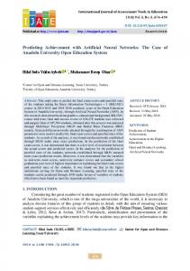
2. Case Description and Methodology The problem described will be analyzed in an energy production plant with the aim of determining the expected electrical generator core-end temperature for a power uprate. The model is developed to estimate, simulate or extrapolate the core-end temperature in a liquid and gas cooled 4-pole [10] [11], electrical generator once the power uprate is finalized. That is the simulation should provide the expected temperature under conditions in which the generator has never operated or being tested. The ultimate reason for this simulation and its results is to verify that type B insulation limits are not exceeded. An example of this type of generators is seen in Figure 1.
2
C. J. Gavilán Moreno
Figure 1. Modeled generator layout.
After defining the problem and determining the equipment (generator) on which power uprate simulations and forecasts will be carried out, it is time to establish the physical model so that target parameters can be known, calculated and extrapolated. Inside the generator there are several physical phenomena: electrical, magnetic, thermal and fluid-mechanical. The phenomenon favoring energy creation inside the generator is the rotation of the magnetic field, which is in turn caused by the electrical phenomenon of rotor turning and subjected to intensity. In this case study, turning speed is considered to be constant. A secondary phenomenon is stator electricity, characterized mostly by phase (3) intensity and terminal voltage. These two phenomena are responsible, together with grid conditions (reactive power), for heat and thermal generation due to parasite processes and losses. Inside the water-and hydrogen-cooled generator there are two heat sinks: one for water and the other for hydrogen. The variables regulating the hydrogen heat sink are hydrogen purity and pressure as they impact the thermal coefficient of the gas, the thermal difference of hydrogen inside the coolers and also hydrogen temperature at the cooler outlet. In the case of coil water, the key variables are coil water flow rate and water temperature in generator inlet and outlet. These variables, which can be seen in Table 1, will be used to develop the model. These parameters will be neural network inputs. The critical part in this type of generators is the core-end, which is exposed to magnetic flux and significant eddy current-induced losses in the tooth tips of the first magnetic plate packs. In this location the cooling effect of the hydrogen and water is not fully developed so the temperature is always higher than any other location. Output variables will be the core-end tooth tip. Table 2 shows the name and location of thermocouples installed in these unfavorable locations. For the purposes of this study, an artificial neural network has been selected as the best method because it is a general tool [12] and therefore works well for both lineal and non-lineal phenomena, hence covering a wide range of possibilities. It is important to take into consideration that the neural network is a universal approximator [13] [14] allowing for generalization and extrapolation [15]. Once the conceptual model, tool and calculation process input and output variables have been determined, it is time to present the model scheme in which calculation stages, acceptance criteria values and admissible error rates will be developed. Figure 2 shows a graphic representation of this process. The process starts by measuring the value of variables in Table 1 and Table 2 under operating conditions in which generator power is below 108.57%. These data are used to test the network based on the following criterion: variable values in Table 1 should allow the network to generate Table 2 values which should be compared to real values to ensure a maximum difference of 0.1˚C. This neural network is used to extrapolate end-core temperature values (Table 2) for a power level of 113.48% of initial rated generator power. Extrapolated values are compared to those obtained when the plant reaches the specific power level. If extrapolation values have a difference of less than 5% compared to plant-measured values, the network is rendered adequate and can be used
3
C. J. Gavilán Moreno
Table 1. Independent variables. Description
Units
Gross generator power
MW
Reactive generator power
MVAR
Generator phase A current
A
Generator phase B current
A
Generator phase C current
A
Generator field voltage
V
Generator field current
A
H2 generator purity
%
H2 generator pressure
KG/CM2
Hydrogen temperature, cooler 1 inlet
˚C
Hydrogen temperature, cooler 1 oulet
˚C
Hydrogen temperature, cooler 2 inlet
˚C
Hydrogen temperature, cooler 2 oulet
˚C
Water temperature, stator inlet coils
˚C
Water temperature, stator outlet coils
˚C
Table 2. Model output variables. Description
Units
Temperature between slots 70 & 71 (tooth tip) TC80
˚C
Temperature between slots 69 & 70 (tooth tip) TC82
˚C
Temperature between slots 68 & 69 (tooth tip) TC84
˚C
Temperature between slots 67 & 68 (tooth tip) TC86
˚C
Temperature between slots 64 & 65 (tooth tip) TC89
˚C
Temperature between slots 63 & 62 (tooth tip) TC93
˚C
for final extrapolation. As previously mentioned, the power uprate value targeted by the licensee is 117.78%, for an apparent power of 1277 MVA and a power factor of 0.95. For end-core temperature value extrapolation, a network entry data sheet needs to be put together, similar to Table 1. Values should include measurements of up to 108.57% plus those measured at the 113.48% stage of initial rated power. The same variables (Table 2) measured under the same conditions, are used to establish network training parameters. In parallel, the values of Table 1 variables are established, as determined by design, for an extended power level of 117.78% (represented in Table 3). Given extrapolation criticality and the stochastic nature of neural networks, this final step will be described in further detail. The neural network will be tested using known data (108.57% and 113.48%). When the point in which the calculated error of end-core temperature values is lower than 0.1˚C, temperature values are calculated in the same point for a power level of 117.78%. In this case, the input variables included in Table 3 will be used as input neural network data. This process will be repeated 30 times, which means that for every point of interest (Table 2), 30 temperature values will be obtained. The expected value will be the average of all of them in each point of interest; temperature values will be determined for a confidence interval of 95%.
3. Model Definition The method based on artificial neural networks provides a solution of acceptable quality with very little effort.
4
C. J. Gavilán Moreno
Figure 2. Flow schematic of the temperature determination process at 117.78% power. Table 3. Variables and values used in the extrapolation to 117.78%. Description
Value
Units
Gross generator power
1150
MW
Reactive generator power
−378
MVAR
Generator phase A current
34940
A
Generator phase B current
34940
A
Generator phase C current
34940
A
Generator field voltage
424
V
Generator field current
5831
A
H2 generator purity
98
%
H2 generator pressure
5.27
KG/CM2
Hydrogen temperature, cooler 1 inlet
52
˚C
Hydrogen temperature, cooler 1 oulet
38
˚C
Hydrogen temperature, cooler 2 inlet
43
˚C
Hydrogen temperature, cooler 2 oulet
38
˚C
Water temperature, stator inlet coils
27.5
˚C
Water temperature, stator outlet coils
45
˚C
5
C. J. Gavilán Moreno
A multilayer neural network (Feedforward) has a feature that was mentioned before: it is a universal approximator. The neural network is conditioned by the input layer, the output layer, as well as the transfer functions that together with the synaptic weights and biases, make up network parameters. Figure 3 shows a proposed network layout. Focusing on the problem under analysis, a multilayer Feedforward network will be adopted. The neural network will have three layers: input, output and hidden. The first layer (input) will have as many neurons as variables in Table 1 [15]. The output layer will have six neurons, one for each output variable included in Table 2. The design of the hidden layer is critical to convergence, error evolution and training performance [16] [17]. The number of neurons in the hidden layer will be selected as follows: • The number of hidden neurons should be in the range between the size of the input layer and the size of the output layer. So the range will be between 15 and 6. • The number of hidden neurons should be 2/3 of the input layer size, plus the size of the output layer. In this particular case they are 16. • The number of hidden neurons should be less than twice the input layer size, so the number should be less than 12. Obviously only the second condition is not coherent with the first and third, therefore, it will be neglected. So finally 12 neurons will be implemented in the hidden layer (see Figure 4).
Figure 3. Typical layout of a Feedforward-type neural network.
Figure 4. Neural network architecture for this model.
6
C. J. Gavilán Moreno
3.1. Training
Once the architecture to be used in a particular problem has been defined, it is necessary to adjust the neural network weight through the training process. The training process is composed of three sub-processes: learning, validation and test. The learning algorithm includes a problem of inference associated to free network parameters and related neuron connections. The learning process of a Feedforward neural network is ought to be supervised because network parameters, known as weights and biases, are estimates based on a set of training patterns (including input and output patterns). In order to estimate network parameters, a backpropagation algorithm is used as generalization of the delta rule proposed by Widrow-Hoff [13] [14]. Learning implies weight adjustment by comparing the neural network output to measured value, to minimize error. The error will be calculated as the mean squared error between the simulated temperature and the real (measured) temperature. Figure 5 shows a detailed training process including three clearly differentiated phases. The first phase is learning as such. In this phase, weights and biases characterizing neurons and their connections are determined by means of the learning process described above. In this phase, 90% of available data is used. After training, it is necessary to determine the error made when comparing network output to actual data and if error is lower than a specific value (0.1˚C in this case), the next phase can be initiated. The second phase is validation. In this phase, output values are calculated using 5% of available data not used during the training phase. If error is less than 0.1, a test is performed and the network rendered “trained”; if the error is not less than 0.1˚C, the learning phase must be repeated until the validation error value meets the target. Figure 6 shows the evolution of the learning error, validation and test. This error estimates how the neural network can be adapted to the problem under analysis. Process results include not only error evolution during the learning phase, but also error distribution throughout the different phases as well as fitting between network-simulated values and real values. These results are specifically addressed in the following section. START
TRAINING
NO ERROR