Using One-Class SVMs and Wavelets for Audio ... - CiteSeerX

1

Using One-Class SVMs and Wavelets for Audio Surveillance Systems Asma Rabaoui∗ , Manuel Davy† , St´ephane Rossignol† , Zied Lachiri∗ and Noureddine Ellouze∗ ∗

Unit de recherche Signal, Image et Reconnaissance des formes, ENIT, BP 37, Campus Universitaire, 1002 le Belvdre, Tunis Tunisia. †

LAGIS, UMR CNRS 8146, and INRIA SequeL Team, BP 48, Cit Scientifique, 59651 Villeneuve d’Ascq Cedex, Lille France.

e-mails:

[email protected],

[email protected]

Abstract This paper presents a procedure aimed at recognizing environmental sounds for surveillance and security applications. We propose to apply One-Class Support Vector Machines (1-SVMs) together with a sophisticated dissimilarity measure as a discriminative framework in order to address audio classification, and hence, sound recognition. We illustrate the performance of this method on an audio database, which consists of above 1,000 sounds belonging to 9 classes. Additionally, the use of a set of state-of-the-art audio features is studied. Additionally, we introduce a set of novel features obtained by combining elementary features. Experimental results are presented and show the superiority of this novel sound recognition method. We show that the 1-SVM clearly overperforms the conventional HMM-based system and we emphasize that the largest improvement is achieved when the system is fed by a set of features that comprises wavelet coefficients. Index Terms Audio surveillance, One-Class SVM, Sounds recognition, Feature combinations, Wavelets.

2

I. I NTRODUCTION Environmental sounds are those sounds which fill our everyday acoustic environment [1]. Recently, some efforts have been directed towards systems capable of detecting and classifying these sounds [1], [2], [3]. The panoply of environmental sounds is vast, it includes the sounds generated in, e.g., domestic, business, and outdoor environments. Hence, most investigations concentrate on a restricted domain. For example, a system able to recognize indoor environmental sounds may be of great importance for surveillance and security applications [3]. These functionalities can also be used in portable tele-assistive devices, to inform disabled and elderly persons affected in their hearing capabilities about specific environmental sounds (door bells, alarm signals, etc.). The system developed in this paper is intended for the recognition of a limited number of classes of environmental sounds and is motivated by a sound-based surveillance application. Such monitoring systems, which are able to classify a number of different environmental sounds related to daily life events, seem to be better accepted by humans than video monitoring. This work forms part of wider investigations about the integration of sound surveillance in monitoring applications. In standard sound recognition approaches [1], [4], [5], [6], [7], [8], the classification of a sound is usually performed in two steps. First, a pre-processor employs Signal Processing techniques to generate a set of features characterizing the signal to be classified. These features form a so-called feature vector. In the space of feature vectors, a decision rule (i.e., a classifier) is then implemented to assign a pattern to a class. During the training phase, the classifier learns how to discriminate between the classes by optimizing some performance criterion with respect to training data. Training data are composed of sounds together with their class labels (which indicate to which class a sound belongs). Once the system has been sufficiently trained for a particular pattern recognition application, its parameters are “frozen” and the classifier is put into service. A key issue is that for successful classification, a good representation of data by audio features is necessary. Results of a given classifier basically depend on the quality of these features: none is a priori good or bad. The quality of a feature has to be analyzed in context of the input data, the application domain, and the sound classes. Similarly, classifiers cannot be evaluated alone; instead, they have to be designed jointly with the features they operate on. In conclusion, a sound classification system should be designed within a given sound context by jointly selecting the set of features and the classifier. A. Previous works Bregman’s book [6] describes a coherent framework for understanding the perceptual organization of sounds. This seminal work has stimulated much interest in computational studies of hearing. Such studies are motivated in part by the need for practical sound separation systems and sound source recognition [4], which have many applications including noise-robust automatic speech recognition [9] and automatic music transcription [10]. This emerging field has become known as computational auditory scene analysis (CASA). Many previous works address CASA. The development of an environmental sound recognition system, in turn, contributes to the development of intelligent machines that are capable of understanding sound. One immediate application is as a core component in a security system [11], [3], [12]. CASA aims at splitting a polyphonic sound source (that may contain speech, but also music and environmental sounds) into separate sounds to be recognized individually using pattern recognition techniques.

3

A full survey of CASA is beyond the scope of this paper, see [13] for a recent overview of the field. Among previous CASA works, we emphasize the emerging research in [14] in the field of speech and speaker recognition, which demonstrates that non-stationary (time-frequency) techniques can be applied to sound classification and can produce good results. Therefore, in [11], [15], [16], [17] both stationary frequency-based techniques and nonstationary time-frequency-based feature extraction techniques were tested in combination with several common classification techniques (traditionally used in speech or in musical instrument recognition) for their suitability to environmental sound recognition. Still in the field of environmental sound recognition, many previous works [1], [2], [9], [18] have focused on recognizing single sound events. Few studies have been reported concerning the broader task of automatic sound recognition when many sound classes are considered. Early works in this vein proposed systems devoted to specific tasks such as sound alerting aid [19], considering some classes of stationary signals (bells, phone, door rings, etc.) and using standard statistical classification procedures based on spectral and temporal features. Later, new classifiers were explored using Hidden Markov Models [20] and Neural Networks [21]. Many other works deal with stationary sounds. For example, ringing sounds classification [22], helicopter noise identification [23], and recognition of music instruments [24] or music types [25]. An extensive thesis was published by Couvreur [1], including a complete bibliographic review of the sound recognition domain and introducing three classifiers for use in separate noise event recognition (car, truck, airplane etc.). Peltonen [2] demonstrated that mel-frequency cepstral coefficients out-performed other feature representations. El-Maleh [9] used various pattern recognition frameworks (such as the Quadratic Gaussian Classifier, Least-Square Linear Classifier, Nearest-Neighbor Classifier, and Decision Tree Classifier), to design noise classification algorithms. Dufaux [12] and Istrate [3] evaluated several audio signal analysis methods using several classifiers and in their works, great interest is devoted to impulsive sound analysis techniques, including traditional time-frequency transformations, speech-typical coefficients and psycho-acoustical features. B. Notations In the remainder of this paper, we adopt the following notations. Let X be the set of training sounds, shared in N classes denoted X1 , . . . , XN . Each class contains mi sounds, i = 1, . . . , N . Sound #j in class Xi is denoted si,j , (i = 1, . . . , N, j = 1, . . . , mi ). Generally, the pre-processor converts a recorded acoustic signal si,j into a

time-localized representation, such as the Short Time Fourier Transform (STFT). Such representations are obtained by splitting the signal si,j into Ti,j overlapping short frames and computing a vector of features zt,i,j , t = 1, . . . , Ti,j with dimension n which characterize each frame. The output of the pre-processor will then be a series of timelocalized features. C. Contributions and paper organization This paper focuses on the applicability of a classifier based on one-class Support Vectors Machines (1-SVMs) in the domain of environmental sound recognition for audio surveillance. Though they have been less studied than two-class SVMs (2-SVMs), 1-SVMs have proved extremely powerful in audio applications [26], [27]. Moreover, we propose to use a set of dedicated audio features, composed of several classical ones together with original waveletbased features. The efficiency of this set of audio features as well as the way they are combined is evaluated and

4

compared to established, standard features. The performance of our technique is evaluated on a data set of sounds collected from the commercial databases [28], [29], which include sounds ranging from screams to explosions, gun shots or glass breaks. The remainder of this paper is organized as follows. Section II gives an overview of the 1-SVM-based sound classifier: pre-processing, 1-SVM theory and introduction of an advanced dissimilarity measure. Section III discusses the advantages of the wavelet-based features and the utility of the 1-SVMs versus other classical frameworks. Experimental set-up and results are provided in Section IV. Section V concludes the paper with a summary and discussion. II. A 1-SVM- BASED

SOUND CLASSIFIER

A. Pre-processing: Features extraction Feature extraction is a key issue when designing an efficient sound recognizer. Perfect features contain all the information relevant to sound classification, are robust to noise while not being corrupted by unnecessary information, and are low-dimensional (generally, this means that features are not correlated with each other). With such features, the type of classifier is not so important. Oppositely, with non-perfect features, the classifier should be selected carefully so as to compensate for the features drawbacks. In this paper, we consider environmental sounds, thus features initially designed for speech seem well adapted. However, environmental sounds may differ significantly from speech, thus we additionally consider features that take care of the possible high non-stationarity of the sounds. Thus, the features selected include those derived from the Fast Fourier Transform (FFT), the Discrete Cosine Transform (DCT) and the Discrete Wavelet Transform (DWT). The advantage of FFT and DCT is that a few coefficients suffice to represent most of the original signal. However, we note that the DWT takes the original signals in time/space domain and transforms them into time/frequency or space/frequency domain, thus keeping the time variable in a natural way. Though some of the features selected are quite standard, we now describe them shortly for completeness, grouped into four categories. 1) Time-domain features: •

The Zero-Crossing Rate (ZCR) is defined as the number of times the sign of a time series st changes within a frame. It roughly indicates the frequency that dominated during that frame. It is defined for the frame t with the length L as: L

ZCR(t) =

1X |sign(st (τ + 1)) − sign(st (τ ))| L

(1)

τ =1

•

The short-time average energy (referred to as “Energy” in the following) is the energy of a frame: Energy(t) =

L−1 1 X |st (τ )|2 L

(2)

τ =0

2) Frequency-domain features: •

The Spectral Centroid (SC) represents the balancing point of the spectral power distribution. It is calculated as the average of the frequencies, weighted by the amplitudes. This is the first moment of the spectrum with

5

respect to frequency. SC is commonly associated with the measure of brightness of a sound. The individual centroid of a spectral frame is defined as: PN −1

kSt [k] SC(t) = Pk=1 N −1 k=1 St [k]

(3)

For the tth frame, St [k] is the magnitude corresponding to the k th frequency and N is the length of the Discrete Fourier Transform (DFT). •

The Spectral Roll-off point (SRF) measures the frequency below which a certain amount of the power spectrum lies. This feature is related to the spectral skewness and it changes for sounds with different frequency ranges. It is calculated by summing up the power spectrum samples until the desired percentage or threshold (referred to as T H below) of the total energy is reached. Considering the DFT of a frame, the SRF is defined as: SRF (t) = max{K\

K X

2

|St (k)| < T H

k=0

where T H is between 0 and 1. The commonly used value is 0.93.

N X

|St (k)|2 }

(4)

k=0

3) Linear Prediction, Perceptual Linear prediction and cepstral features: These features are used to describe the spectral shape of a signal. •

The Mel-Frequency Cepstral Coefficients (MFCCs) are extracted by applying the discrete cosine transform to the log-energy outputs of mel-scaling filter-bank [30].

•

Linear Prediction Cepstral Coefficients (LPCCs) are extracted using the autocorrelation method [31]. Given the linear predictive coefficients ak , k = 1, . . . , N , see [32], the Linear Predictive Cepstral Coefficients (LPCCs) are determined by the following recursive relationship: ( c1 = a 1 , P k cn = n−1 k=1 (1 − n )an cn−k + an , n = 1, . . . , P

(5)

where P ≤ N is the desired number of cepstral coefficients. •

Perceptual Linear Prediction analysis (PLP) is a variation of the original linear prediction analysis. The main idea of this technique is to take advantage of three main psycho-acoustical properties of the human ear for estimating the audible spectrum, namely: spectral resolution of the critical band, equal-loudness curve and intensity-loudness power law. PLP maps the linear prediction spectrum to the nonlinear frequency scale of the human ear. The perceptual linear prediction coefficients (PLPCC) are an extension of the LPCCs. In its original formulation, PLPCCs are not robust to signal distortion. By employing a RASTA (Relative Spectral) filter [33], PLP analysis becomes more robust to distortion. The resulting technique is called RASTA PLP analysis which consists in a special filtering of the different frequency channels of a PLP analyzer. The RASTA method replaces the conventional critical-band short-term spectrum in PLP and introduces a less sensitive spectral estimation. RASTA PLP makes PLP more robust to linear spectral distortions.

4) Wavelet-based features: We propose a new set of wavelet-based feature vectors, derived from wavelet coefficients. The wavelet coefficients capture time and frequency localized information about the sound waveform that standard Fourier analysis cannot capture: Different from Fourier-based analysis, Wavelet Transforms (WT) use short duration basis functions to measure the signal high frequency content and long duration basis functions for low frequency content (constant-Q analysis) [34].

6

The WT actually implements a bank of filters, which are scaled versions of a prototype filter ψ(t) given by: 1 τ ψτ,a (t) = a− 2 ψ(t − ), ψ ∈ L2 (L2 is a finite energy space) a

(6)

where parameters τ and a are called translation and scaling parameters respectively. The term a −1/2 is used for energy normalization. The DWT of a signal s can be obtained as: X D(j, k) = 2−j/2 s(i)ψ ∗ (2−j i − k)

(7)

i

where i, j and k are integers and ·∗ denotes complex conjugation. By choosing the scaling factor as dyadic (2j ) the resultant transform is known as dyadic DWT. If the wavelet decomposition is computed up to a scale 2 j , the

resultant signal representation is not complete. The lower frequencies corresponding to scales larger than 2 j must also be computed and added. These lower frequency components can be evaluated by using the following equation: X A(j, k) = 2−j/2 s(i)φ∗ (2−j i − k) (8) i

where

φ∗ (i)

is the complex conjugate of the scaling function φ(i).

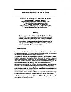
The DWT can be viewed as the process of filtering the signal using a low pass (scaling) filter and high pass (wavelet) filter. Thus, the first layer of the DWT decomposition of a signal splits it into two bands giving a low pass version and a high pass version of the signal. The low pass signal gives the approximate representation of the signal while the high pass filtered signal gives the details or high frequency variations. The second level of decomposition is performed on the low pass signal obtained from the first level of decomposition (as shown in Fig .1). Thus a wavelet decomposition results in a binary tree like structure which is left recursive (where the left child usually represents the lower frequency band). The wavelet decomposition of the signal S analyzed at level j has the following structure: [cAj , cDj , . . . , cD1 ].

Fig. 1.

Block diagram of the dyadic discrete wavelet transform (DWT).

For more information about the Wavelet Transform (WT) and its implementations, interested readers may refer to [35], [34]. In this paper, we consider two approaches based on WTs. The main idea of the first approach was introduced in [36], [37], [38], where the WT is applied to a speech signal, and the WT sub-band energies replace the Mel filterbank sub-bands energies. By using this approach the time information in the wavelet sub-bands is lost into the sub-band energies. Our approach differs in that we use the actual wavelet coefficients, and not the sub-band energies. This retains the time information.

7

Another approach that uses the wavelet transform consists of using it instead of the cepstrum [39], [40], [41]: Mel filterbank sub-band energies are computed, the log is taken, and then a Discrete Wavelet Transform (DWT) is performed. The features obtained are called the Mel Frequency Discrete Wavelet Coefficients (MFDWCs). 5) Features normalization: After the features are extracted, they should be normalized in order to avoid that the typical amplitude of one feature is one or two orders of magnitude larger than that of another feature. When forming feature vectors, and comparing them with standard distances such as the Euclidean, the largest amplitude features dominate, and the others have no influence. This explains why feature normalization is required. We consider the following simple second order normalization technique applied to a n-dimensional feature vector, zˆ = (z − µ) · /σ , where z and zˆ are the original and normalized feature vectors, respectively, and µ and σ are the

mean and standard deviation vectors (·/ is the term-by-term division). Supposing that one n-dimensional feature vector zt = [zt1 , . . . , ztn ] is extracted from the tth frame. Then, for T frames, the features can be presented in the form of an observation matrix M = [z1 , z2 , . . . , zT ] of dimension n × T . This set of frames can be used to estimate P the global mean vector µ given by µ = [µ1 , µ2 , . . . , µn ] with the mean elements µi = [ Tt=1 zti ]/T for each feature 1 2 n i dimension i = 1, . . . , n. Similarly, the global variance q P vector σ is given by σ = [σ , σ , . . . , σ ] and the variance σ in the ith features dimension is given by σ i = [ Tt=1 (zti − µi )2 ]/(T − 1). The normalization consists of scaling

the feature range in each dimension i, to get zero mean values and unit variances.

6) Feature combinations: As mentioned above, the sound classification performance is quite dependent on the set of features selected. In order to approach the perfect feature set, we propose to combine the above features by including them, or not, into the feature vector used to perform classification. Our approach is different from the commonly used feature selection process which consists of choosing a maximal informative subset from a given set of features. Statistical methods, such as the Principal Component Analysis (PCA) [42] that maximizes the variance among the features, are often applied for feature selection. Besides, PCA can be used to generate new features based on existing ones [43]. In this paper, the proposed method is not dealing with features selection but with feature vectors selection. It consists of evaluating several feature vectors separately and selecting the most performing ones for use as elementary feature vectors which are provided by basic Signal Processing transforms (such as DWT, DCT and FFT). Then, to each selected elementary vector, is added a set of other feature vectors and the performance of the resulting feature vector is evaluated. The empirical research for an optimal solution is described in Algorithm 2 in Section II-E. The classification of such feature vectors requires a classification technique adapted to large dimensional data shared into many classes. The approach we present below relies on an original combination of several one-class SVMs (1-SVMs), which can practically deal with large dimensional data. Before describing the approach, it is necessary to reduce the feature vector description of all the signals (with different durations) to a fixed dimensional vector. 7) Handling sounds signals with different durations: An important problem when considering real sounds is that the time series have different lengths. In order to use SVM classifiers, we must encode the waveform information into a fixed-length vector. Furthermore, it is important to consider the nonstationarity as it may carry discriminant information. A simple but effective approach used in most state-of-the-art speech recognition systems is to assume that the sound signals are composed of a fixed number of sections [44], [45], [46]. Though the sounds considered here have time and frequency characteristics that may differ significantly from those of speech sounds, we have found

8

that a similar technique could be used. We propose to convert each signal s from its waveform representation into a sequence of feature vectors by first splitting it into T overlapping short frames (where T depends on the duration of s) and then computing a vector of features zt , with dimension d which characterize each frame t = 1, . . . , T . Then, the frames are shared into three portions (P1 , P2 and P3 ) with durations proportional to 3-4-3, and construct P a composite 3n dimensional vector from the mean vectors of the three regions, xi = [ Pi zt ]/Ii , ∀i ∈ {1, 2, 3}, where each region Pi is represented by the indexes of the Ii frames contained in it, see Fig .2.

Fig. 2. Composite vector construction for a sound signal s. Starting from the time series of T feature vectors in dimension n, their means are computed over three regions with length proportional to 3-4-3, and grouped into a single composite vector with dimension 3n.

B. The One-class Approach The 1-SVM approach1 [51] has been successfully applied to various learning problems [27], [52], [53], [54], [46]. It consists of learning the minimum volume contour that encloses most of the data in a dataset. Its original application is outlier detection, to detect data that differ from most of the data within a dataset. More precisely, let X = {x1 , . . . , xm } a dataset in Rd . Here, each xj is the full feature vector of a signal, i.e., each signal is represented by one vector xj in Rd , with d = 3n. The aim of 1-SVMs is to use the training data so as to learn a function fX : Rd 7→ R such that most of the data in X belong to the set RX = {x ∈ Rd with fX (x) ≥ 0} while the volume of RX is minimal. This problem is termed minimum volume set (MVS) estimation,

see [55], and we see that membership of x to RX indicates whether this datum is overall similar to X , or not. 1

Various terms have been used in the literature to refer to one-class learning approaches. The term single-class classification originates

from Moya [47], but also outlier detection [48], novelty detection [26], [49] or concept learning [50] are used.

9

Thus, by learning regions RXi for each class of sound (i = 1, . . . , N ), we learn N membership functions fXi . Given the fXi ’s, the assignment of a datum x to a class is performed as detailed in Section II-C. 1-SVMs solve MVS estimation in the following way. First, a so-called kernel function k(·, ·) ; R d × Rd 7→ R is selected, and it is assumed positive definite, see [51]. Here, we assume a Gaussian RBF kernel such that £ ¤ k(x, x0 ) = exp − kx − x0 k2 /2σ 2 , where k · k denotes the Euclidean norm in Rd . This kernel induces a so-called

feature space2 denoted H via the mapping φ : Rd 7→ H defined by φ(x) , k(x, ·), where H is shown to be reproducing kernel Hilbert space (RKHS) of functions, with dot product denoted h·, ·iH . The reproducing kernel property implies that hφ(x), φ(x0 )iH = hk(x, ·), k(x0 , ·)iH = k(x, x0 ) which makes the evaluation of k(x, x0 ) a linear operation in H, whereas it is a nonlinear operation in Rd . In the case of the Gaussian RBF kernel, we see that kφ(x)k2H , hφ(x), φ(x)iH = k(x, x) = 1, thus all the mapped data are located on the hypersphere with radius one, centered onto the origin of H denoted S(o,R=1) , see Fig 3. The 1-SVM approach proceeds in feature space by determining the hyperplane W that separates most of the data from the hypersphere origin, while being as far as possible from it. Since in H, the image by φ of RX is included in the segment of hypersphere bounded by W , this indeed implements MVS estimation [55]. In practice, let W = {h(·) ∈ H with hh(·), w(·)i H − ρ = 0} , then its parameters w(·) and ρ results from the optimization problem m

1 1 X min kw(·)k2H + ξj − ρ w,ξ,ρ 2 νm

(9)

j=1

subject to (for i = 1, . . . , m) hw(·), k(xj , ·)iH ≥ ρ − ξj ,

and ξj ≥ 0

(10)

where ν tunes the fraction of data that are allowed to be on the wrong side of W (these are the outliers and they do not belong to RX ) and ξj ’s are so-called slack variables. It can be shown [51] that a solution of (9)-(10) is such that w(·) =

m X

αj k(xj , ·)

(11)

j=1

where the αj ’s verify the dual optimization problem m 1 X min αj αj 0 k(xj , xj 0 ) α 2 0

(12)

j,j =1

subject to 0 ≤ αj ≤

Finally, the decision function is fX (x) =

1 , νm

m X

X

αj = 1

(13)

αj k(xj , x) − ρ

(14)

j

j=1

and ρ is computed by using that fX (xj ) = 0 for those xj ’s in X that are located onto the boundary, i.e., those that verify both αj 6= 0 and αj 6= 1/νm. An important remark is that the solution is sparse, i.e., most of the αi ’s are zero (they correspond to the xj ’s which are inside the region RX , and they verify fX (x) > 0). 2

We stress on the difference between the feature space, which is a (possibly infinite dimensional) space of functions, and the space of

feature vectors, which is Rd . Though confusion between these two spaces is possible, we stick to these names as they are widely used in the literature.

10

As plotted in Fig. 3, the MVS in H may also be estimated by finding the minimum volume hypersphere that encloses most of the data (Support Vector Data Description (SVDD) [54]), but this approach is equivalent to the hyperplane one in the case of a RBF kernel.

Fig. 3.

In the feature space H, the training data are mapped on a hypersphere S (o,R=1) . The 1-SVM algorithm defines a hyperplane with

equation W = {h ∈ H s.t. hw, hiH − ρ = 0}, orthogonal to w. Black dots represent the set of mapped data, that is, k(x j , ·), i = 1, ..., m. For RBF kernels, which depend only on x − x0 , k(x, x0 ) is constant, and the mapped data points thus lie on a hypersphere. In this case, finding the smallest sphere enclosing the data is equivalent to maximizing the margin of separation from the origin.

In order to adjust the kernel for optimal results, the parameter σ can be tuned to control the amount of smoothing, i.e. large values of σ lead to flat decision boundaries, as shown in Fig. 4. Also, ν is an upper bound on the fraction of outliers in the dataset [51]. Fig. 4 displays an example of a 2-dimensional data to which a 1-SVM using an RBF kernel was applied for different values of ν and σ .

Fig. 4.

A Single-class SVM using an RBF kernel is applied to a 2-dimensional data; the parameter ν characterizes the fractions of SVs

(Support Vectors) and outliers (points which are on the wrong side of the hyperplane). The parameter σ characterizes the kernel width. For these plots, the parameters are (a) ν = 0.1, σ = 1 (b) ν = 0.3, σ = 1 (c) ν = 0.3, σ = 4.

11

C. A dissimilarity measure The 1-SVM described above can be used to learn the MVS of a dataset of feature vectors which relate to sounds. This is not yet a multiclass classifier, and we now describe how to build such a classifier, by adapting the results of [27], [56]. Assume that N 1-SVMs have been learnt from the datasets {X1 , . . . , XN }, and consider one of them, with associated set of coefficients denoted ({αj }j=1,...,m , ρ). In order to determine whether a new datum x is similar to the set X , we define a dissimilarity measure, denoted d(X , x) as follows d(X , x) = − log[

m X

αj k(x, xj )] + log[ρ]

(15)

j=1

in which ρ is seen as a scaling parameter which balances the αj ’s. Thanks to this normalization, the comparison of such dissimilarity measures d(Xi , x) and d(Xi0 , x) is possible. Indeed, ¡ ¢¤ £ hw(·), k(x, ·)iH ¤ £ kw(·)kH cos w(·)∠k(x, ·) d(X , x) = − log = − log ρ ρ

(16)

because kk(x, ·)kH = 1, where w(·)∠k(x, ·) denotes the angle between w(·) and k(x, ·). By doing elementary ρ b , see Fig.3. This yields the following interpretation = cos(θ) geometry in feature space, we can show that kw(·)kH

of d(X , x)

¡ ¢ £ cos w(·)∠k(x, ·) ¤ d(X , x) = − log b cos(θ)

(17)

which shows that the normalization is sound, and makes d(X , x) a valid tool to examine the membership of x to a given class represented by a training set X .

D. Multiple sound classes 1-SVM-based classification Algorithm The sound classification algorithm comprises three main steps. Step one is that of training data preparation, and it includes the selection of a set of features which are computed for all the training data. The value of ν is selected in the reduced interval [0.05, 0.8] in order to avoid edge effects for small or large values of ν . Algorithm 1: Sound classification algorithm Step 1: Data preparation •

Select a set of features among those presented in Subsection II-A

•

Form the training sets Xi = {xi,1 , ..., xi,mi }, i = 1, . . . , N by computing these features and forming the feature vectors for all the training sounds selected.

•

Set the parameter σ of the Gaussian RBF kernel to some pre-determined value (e.g., set σ as half the average euclidean distance between any two points xi,j and xi0 ,j 0 , see [57]), and select ν ∈ [0.05, 0.8].

Step 2: Training step •

For i = 1, . . . , N , solve the 1-SVM problem for the set Xi , resulting in a set of coefficients (αi,j , ρj ), j = 1, . . . , mi

Step 3: Testing step •

For each sound s to be classified into one of the N classes, do – compute its feature vector, denoted x, – for i = 1, . . . , N , compute d(Xi , x) by using Eq. (15)

12

– assign the sound s to the class bi such that bi = arg mini=1,...,N d(Xi , x)

E. Parameters optimization and feature selection The above algorithm requires the selection of parameters ν and σ , as well as a set of features. For a sufficiently large training set, it is possible to select the optimal set by applying an original cross-validation procedure [58], as described in Algo. 2. Note that the value of ν is not learnt, as this may lead to overfitting. Throughout all this study, we have kept ν = 0.2. Algorithm 2: Optimization procedure for the parameters and feature combinations •

Step 0: Initialization – Select an initial combination of features – Select ν

•

Step 1: Iterations – Add or remove one feature from the combination, resulting in a new set of features – for p = 1, . . . , P , do ∗ For i = 1, . . . , N , randomly split Xi in two approximately equal parts denoted Xi1 and Xi2 respectively. ∗ Evaluate the value of σ by using the rule of Algorithm 1 ∗ Compute the N 1-SVMs for the sets {X11 , . . . , XN1 } ∗ For each datum x in {X12 , . . . , XN2 }, compute d(Xi1 , x) for i = 1, . . . , N and assign x to the class that minimizes d(Xi1 , x) ∗ Evaluate Ep , the number of missclassifications (i.e., the number of data assigned to a class they do not belong to) – compute the average number of errors E =

£ PP

p=1

¤ Ep /P

III. D ISCUSSION The algorithm presented below has several original aspects, the most prominent being the use of several 1-SVMs to perform multiple classes classification and the use of wavelet-based audio features. A. On the use of several 1-SVMs to perform multi-class classification Machine learning has recently seen a number of works about multi-class classification by using SVMs. Most of these works aim at designing either a direct multiple classes algorithm which requires a unique global training step, or try to split the problem into several two classes sub-problems. These approaches are generally quite precise when the number of classes is small (typically up to 5), and when the number of training data is reasonable. Indeed, all the data ¢ ¡PN PN 3 to of all classes are used to train the multiclass-SVM, which scales typically from O i=1 i0 =1,...,N (mi + mi0 ) i0 6=i ¢ ¡P 3 . However, the 1-SVM approach can be generalised to any number of classes, and the computational m ) O ( N i=1 i ¡ PN ¢ 3 cost for training scales with O i=1 mi , which may be far quicker than any of the multiple class approaches.

Also, the application addressed here concerns sound classification. In real environment, there might be many

sounds which do not belong to one of the pre-defined classes, thus it is necessary to define a rejection class, which

13

may gather all sounds which do not belong to the training classes. An easy and elegant way to do so consists of estimating the regions of high probability of the known classes in the space of features, and considering the rest of the space as the rejection class. Training several 1-SVMs does this automatically, and a sound with feature vector x is (optionally) assigned to the rejection class whenever d(Xi , x) > η for all i, where η is a rejection threshold

tuned by the user.

B. SVMs vs. Common Classifiers In a number of problems, SVMs have been shown to have important advantages over more traditional techniques. For SVMs, few parameters need to be tuned, the optimization problem to be solved does not have numerical difficulties – mostly because it is convex. Moreover, their generalization ability is easy to control through the parameter ν , which admits a simple interpretation in terms of the number of outliers, see [51]. In audio recognition and especially speech recognition, the most popular approach is based on Hidden Markov Models (HMMs) with Gaussian mixture observation densities. These systems typically use a representational model based on maximum likelihood decoding and expectation maximization-based training. Though powerful, this paradigm is prone to overfitting and does not directly incorporate discriminative information. It is shown that HMMbased sounds recognition systems perform very well on closed-loop tests but performance degrades significantly on open-loop tests. In [59], we showed that this is specially true for impulsive sounds classification. As an attempt to overcome these drawbacks, Artificial Neural Networks (ANNs) have been proposed as a replacement for the Gaussian emission probabilities under the belief that the ANN models provide better discrimination capabilities. However, the use of ANNs often results in over-parametrized models which are also prone to overfitting. Overall, we found the 1-SVM methodology more easy to implement and tune and well adapted to large dimensional feature vectors, while having a reasonable training cost.

C. On the use of wavelet-based features Features based on standard sliding window Fourier analysis implicitly assume that the analyzed signal is stationary over each window. However, in the case of surveillance sound signals, impulsive events are often met, and the local stationarity assumption is inaccurate. One could select a short duration window, but this makes the frequency resolution poor, due to the Heisenberg-Gabor inequality [60]. By using wavelets, which somehow implements multiple time resolution analysis, two very short bursts can be separated in time by going to the high frequencies. Therefore, this analysis can be used for the signals which have short-duration high-frequency components and long-duration low-frequency components. This is indeed a property of most impulsive sounds. IV. E XPERIMENTAL

SET- UP AND EVALUATIONS

In this section, we first describe the database used to evaluate the sound classification system. Then, we provide the implementation details as well as values for the algorithm parameters. Then, we present the results obtained, and compare them to the celebrated HMM/GMM classifier.

14

A. Database description The major part of the sound samples used in the recognition experiments is taken from different sound libraries available [29], [28]. Considering several sound libraries is necessary for building a representative, large, and sufficiently diverse database. Some particular classes of sounds have been built or completed with signals recorded by us. All signals in the database have a 16 bits resolution and are sampled at 44100 Hz, enabling a good time resolution and wide frequency band, which are both necessary to cover harmonic as well as impulsive sounds. During database construction, great care was devoted to the selection of the signals. When a rather general use of the recognition system is required, some kind of intra-class diversity in the signal properties should be integrated in the database. As a result, each class includes sounds with very different temporal or spectral characteristics, amplitude levels, duration and time alignment. The selected sound classes are given in Tab. I, and they are typical of a surveillance application. TABLE I C LASSES OF SOUNDS AND NUMBER OF SAMPLES IN

THE DATABASE USED FOR PERFORMANCE EVALUATION .

Classes

Class number

Train

Test

Total

Human screams

C1

48

25

73

Gunshots

C2

150

75

225

Glass breaks

C3

58

30

88

Explosions

C4

41

21

62

Door slams

C5

209

105

314

Dog barks

C6

36

19

55

Phone rings

C7

34

17

51

Children voices

C8

58

29

87

Machines

C9

40

20

60

674

341

1015

Total

An important remark about this database is that it includes both impulsive sounds classes and harmonic sounds such as phone rings (C7) and Children voices (C8). These have been considered as these sounds are quite likely to be recorded by a surveillance system, while not necessary being related to an emergency situation. A proper surveillance system should be able to correctly recognize these sounds, in order to have few false alarms. Another remark is that some classes of sounds are very close for human listeners. In particular, Explosions (C4) are pretty similar to Gunshots (C2). The system should be able to discriminate sounds from these classes.

B. Results with individual features In order to enlight the usefulness of the features presented in Subsection II-A, we first present classification results obtained when retaining only one feature in the feature vector, and applying Algo 1. Features are computed from all the samples in each sound. The analysis window in Hamming with length 25 ms and 50 % overlap. The feature vectors are formed and normalized as explained in Subsection II-A. Concerning wavelet-based features, the Daubechies wavelets with 4 vanishing moments are used. This family of wavelets has minimum support size of 2ζ − 1 for a given number of vanishing moments ζ . These compactly supported wavelet filters are designed by using a finite impulse response conjugate mirror filter [35].

15

Based on preliminary experiments, we noticed that adding the first and second derivatives of the features had negligible effects on the performance. Evaluations on the 1-SVM-based system (using a Gaussian RBF kernel) with individual features are compared to the results obtained by the baseline HMM-based classifier with 3 hidden states and 3 Gaussians components in each state (whose parameters are learnt by 5 iterations in the Baum-Welch algorithm [61], [62]). Tab. II provides the results obtained by the two techniques, where the performance rate is computed as the percentage number of sounds correctly recognized and it is given by (H/N) × 100%, where H is the number of correct sounds and N is the total number of sounds to be recognized. No results are proposed for the HMM classifier fed by the Wavelet-based coefficients, as these features have too large dimension to enable GMM modelling. TABLE II R ECOGNITION RATES USING VARIOUS INDIVIDUAL FEATURES APPLIED TO 1-SVM S AND HMM S BASED CLASSIFIERS . Recognition rate (%) Features

1-SVM

HMM

P LP C

88.82

88.73

LP CC

91.56

90.46

M F CC

92.8

91.69

DW C

72.22

—-

M F DW C

78.93

82.15

RAST A P LP C

90.22

89.23

The results in Tab. II show that the 1-SVM performs slightly better in almost all the cases. Another remark is that non of the individual features is able to achieve very high performance. This justifies the use of combinations of features, as exposed in the next subsection. C. Results with combinations of features In this section, results obtained with various feature combinations are discussed. We illustrate that different feature combinations can lead to quite different performance, see Tab. III, where the combinations displayed are obtained by including incrementally in the combinations other features that are known to be little correlated with the already selected ones (feature correlations has been investigated in many previous works, see [12], [63], [64] for instance). The results for each combination are evaluated by the 1-SVM-based classifier and compared to the results of the HMM-based classifier. Tab.’s IV–VII present the confusion matrices for several of the feature combinations of Tab. III, for the 1-SVM multi-class classifier. D. Comments and discussion In [64], it is shown that the information of LPC coefficients is already captured by the more expressive MFCCs. Our experiments confirm this conclusion. This is also true for PLP features. Hence, we do not include LPC and PLP coefficients in the combination whenever MFCCs are already included. For highly redundant groups of features we choose only individual representative components. [12] shows that adding temporal features can improve the classification performance. Thus, we added ZCR and the average energy which are one-dimensional features. ZCR

16

TABLE III R ECOGNITION RATES FOR VARIOUS FEATURES COMBINATIONS APPLIED TO 1-SVM S AND HMM S BASED CLASSIFIERS . Coefficients Number Features

Recognition Rate

(per frame)

SVM

HMM

MFCC + Energy + Log energy

14

92.89

91.22

MFCC + Energy + Log energy + SRF + SC

16

93.79

91.89 89.15

PLPCC + Energy + Log energy

14

93.99

RASTA PLP + Energy + SRF + SC + ZCR

16

94.22

89.48

LPCC + Energy + Log energy + SRF + SC + ZCR

17

92.45

90.89

MFDWC + Energy + SRF + SC + ZCR

16

87.48

85.33

DWC + Energy + SRF + SC + ZCR

115

86.80

—-

DWC + MFCC + Energy + Log energy + SRF + SC + ZCR

117

96.89

—-

TABLE IV C ONFUSION M ATRIX OBTAINED BY USING A L OG

ENERGY

FEATURE VECTOR CONTAINING

12

CEPSTRAL COEFFICIENTS

MFCC + E NERGY +

+ SC + SRF. 1-SVM S ARE APPLIED WITH AN RBF KERNEL (σ =10).

C1

C2

C3

C4

C5

C6

C7

C8

C9

C1

100

0

0

0

0

0

0

0

0

C2

0

90.66

0

9.33

0

0

0

0

0

C3

0

0

93.33

0

6.66

0

0

0

0

C4

0

20.05

0

75.19

4.76

0

0

0

0

C5

0

0.95

0

1.9

97.14

0

0

0

0

C6

0

0

0

0

5.26

94.73

0

0

0

C7

0

0

0

0

0

0

100

0

0

C8

0

0

0

3.45

3.45

0

0

93.1

0

C9

0

0

0

0

0

0

0

0

100

Total Recognition Rate = 93.79% TABLE V C ONFUSION M ATRIX OBTAINED BY USING A L OG

ENERGY

FEATURE VECTOR CONTAINING

12

CEPSTRAL COEFFICIENTS

LPCC + E NERGY +

+ SRF + SC + ZCR. 1-SVM S ARE APPLIED WITH AN RBF KERNEL (σ =12). C1

C2

C3

C4

C5

C6

C7

C8

C9

C1

100

0

0

0

0

0

0

0

0

C2

0

82.66

0

14.66

2.67

0

0

0

0

C3

0

10

82.33

7.66

0

0

0

0

0

C4

0

10.04

0

85.19

4.76

0

0

0

0

C5

0

2.86

0

3.81

81.9

1.9

0

9.52

0

C6

0

0

0

0

0

100

0

0

0

C7

0

0

0

0

0

0

100

0

0

C8

0

0

0

0

0

0

0

100

0

C9

0

0

0

0

0

0

0

0

100

Total Recognition Rate = 92.45%

is closely related to the fundamental frequency over a frame. In the case of environmental sounds the fundamental frequency may be similar for different classes; this is why ZCR is not suited to classification as a single feature.

17

TABLE VI C ONFUSION M ATRIX OBTAINED BY USING A L OG

ENERGY.

FEATURE VECTOR CONTAINING

12

CEPSTRAL COEFFICIENTS

PLPCC + E NERGY +

1-SVM S ARE APPLIED WITH AN RBF KERNEL (σ =10)

C1

C2

C3

C4

C5

C6

C7

C8

C9

C1

100

0

0

0

0

0

0

0

0

C2

0

82.66

2.66

13.33

1.33

0

0

0

0

C3

0

0

93.33

0

6.66

0

0

0

0

C4

0

19.05

0

76.66

4.76

0

0

0

0

C5

0

0

4.76

1.9

93.33

0

0

0

0

C6

0

0

0

0

0

100

0

0

0

C7

0

0

0

0

0

0

100

0

0

C8

0

0

0

0

0

0

0

100

0

C9

0

0

0

0

0

0

0

0

100

Total Recognition Rate = 93.99% TABLE VII C ONFUSION M ATRIX OBTAINED BY USING A FEATURE VECTOR CONTAINING DWC (DAUBECHIES OF MOMENT 4 DECOMPOSITION LEVEL =7, ABOVE

100

COEFFICIENTS ARE USED )

+ 12 MFCC + E NERGY + L OG

ENERGY

WITH

+ SRF + SC + ZCR.

1-SVM S ARE APPLIED WITH AN RBF KERNEL (σ =2) C1

C2

C3

C4

C5

C6

C7

C8

C9

C1

100

0

0

0

0

0

0

0

0

C2

0

97.66

0

2.33

0

0

0

0

0

C3

0

0

96.33

0

3.66

0

0

0

0

C4

0

9.05

0

86.19

4.76

0

0

0

0

C5

0

0.95

0

1.9

97.14

0

0

0

0

C6

0

0

0

0

5.26

94.73

0

0

0

C7

0

0

0

0

0

0

100

0

0

C8

0

0

0

3.45

3.45

0

0

100

0

C9

0

0

0

0

0

0

0

0

100

Total Recognition Rate = 96.89%

Due to the low-dimension of the tested temporal features (ZCR and the average energy) and the frequency features (SRF and SC), they fail to represent data information. Nevertheless, these features may improve retrieval quality in combination with the preselected basis features (as showed in Subsection II-A). In general, combinations involving spectral and time-based features are useful, since they combine information of the two complementary domains: while spectral features characterize the frequency contents, time-based features incorporate temporal information and loudness. The results in Tab. II show that some features are not able to discriminate between the classes successfully when used alone. The DWT coefficients do not separate well some classes. This can be partly explained by the fact that DWT coefficients are mostly informative for low frequencies, and they tend to neglect high frequencies. This justifies the use of 12 MFCCs in addition to DWT coefficients. As can be seen in Tab. VII, this significantly improves the discrimination ability. The use of 1-SVMs is plainly justified by the results presented here, as it yields consistently lower error rates and

18

a high classification accuracy for the major part of the feature combinations. It appears that the most informative feature combinations have large dimension, which does not allow the use of GMMs/HMMs techniques. 1-SVMs, by mapping the data in the feature space, are less sensitive to the dimension d of the data space, thus they permit the use of these informative feature combinations. Some additional conclusions about the tests presented here are: •

While simple features, such as coefficients of basic time/frequency transforms (DFT, DWT, and DCT), are not able to capture discriminative properties of the classes, features of high complexity, such as cepstral coefficients, are well suited for recognition of environmental sounds.

•

Beside the complexity, the classification accuracy often depends on the dimensionality of the features. While low-dimensional features, such as cepstral parameters are limited by their expressiveness in distinguishing some very close sounds classes (guns and explosions) (as seen in all Tab.’s IV–VII), combination with highdimensional features (wavelet components) provide more discrimination performance (Tab. VII). V. C ONCLUSION

The system developed in this paper is intended for the recognition of given classes of environmental sounds and is motivated by a practical surveillance application. The proposed system uses a discriminative method based on one-class SVMs, together with a sophisticated dissimilarity measure, in order to classify a set of sounds into predefined classes. The efficiency of various acoustic features as well as the influence of features combinations were studied. More research is needed on understanding how 1-SVMs can be useful for sounds classification under very noisy conditions. Hence, to successfully develop sounds recognition applications, it is crucial to take into account such discrepancies. This can be achieved using different kinds of techniques aiming essentially at finding robust and invariant signal features using adaptation methods or robust decision strategies. R EFERENCES [1] C. Couvreur, “Environmental Sound Recognition: A Statistical Approach,” Ph.D. dissertation, Facult e´ Polytechnique de Mons, Belgium, June 1997. [2] V. Peltonen, “Computational auditory scene recognition,” Ph.D. dissertation, Tampere University of Technology, Finland, 2001. [3] D. Istrate, “Dtection et reconnaissance des sons pour la surveillance mdicale,” Ph.D. dissertation, INPG, France, Dec. 2003. [4] K. D. Martin, “Sound-source recognition: A theory and computational model,” Ph.D. dissertation, MIT Press, 1999. [5] G. J. Brown and M. Cooke, “Computational Auditory Scene Analysis,” Computer Speech and Language, vol. 8, pp. 297–336, 1994. [6] A. Bregman, Auditory scene analysis. Cambridge, USA: MIT Press, 1990. [7] D. P. W. Ellis, “Prediction-driven computational auditory scene analysis,” Ph.D. dissertation, MIT Press, 1996. [8] M. P. Cooke, Modeling auditory processing and organisation. Cambridge, UK: Cambridge University Press, 1993. [9] K. El-Maleh, “Frame level noise classification in mobile environments,” Ph.D. dissertation, McGill University, Montreal, Canada, Jan. 2004. [10] A. Klapuri and M. Davy, Eds., Signal Processing Methods for Music Transcription. New York: Springer, 2006. [11] M. Cowling, “Non-speech environmental sound classification system for autonomous surveillance,” Ph.D. dissertation, Faculty of Engineering and Information Technology, Griffith University, 2004. [12] A. Dufaux, “Detection and recognition of Impulsive Sounds Signals,” Ph.D. dissertation, Facult e´ des sciences de l’Universit´e de Neuchˆatel, Switzerland, 2001. [13] D. Wang and G. J. Brown, Computational Auditory Scene Analysis: Principles, Algorithms and Applications. Ltd, 2007.

John Wiley and Sons

19

[14] M. Orr, D. Pham, B. Lithgow, and R. Mahony, “Speech perception based algorithm for the separation of overlapping speech signal,” in The Seventh Australian and New Zealand Intelligent Information Systems Conference, 2001. [15] M. Cowling and R. Sitte, “Sound identification and direction detection for surveillance applications,” in ICICS, 2001. [16] ——, “Recognition of environmental sounds using speech recognition techniques,” Advanced Signal Processing for Communications Systems, 2002. [17] ——, “Comparison of techniques for environmental sound recognition,” Pattern Recognition Letters, vol. 24, pp. 2895–2907, 2003. [18] R. S. Goldhor, “Recognition of environmental sounds,” in ICASSP, vol. 1, New York, USA, 1993, pp. 149–152. [19] B. Uvacek, H. Ye, and G. Moschytz, “A new strategy for tactile hearing aids: tactile identification of preclassified signals (tips),” in International Conference on Acoustic, Speech and Signal Processing (ICASSP), New-York, USA, May 1988. [20] A. K. S. Oberle, “Recognition of acoustical alarm signals for the profoundly deaf using hidden Markov models,” in International Symposium on Circuits and Systems, vol. 1, Seattle, USA, 1995, pp. 2285–2288. [21] J. A. Osuna and G. S. Moschytz, “Recognition of acoustical alarm signals with cellular networks,” in European Conference on Circuit Theory and Design, Istanbul, Turkey, 1995. [22] M. J. Paradie and S. Nawab, “Classification of ringing sounds,” in ICASSP, Apr. 1990. [23] R. H. Cabell, C. Fuller, and W. O’Brien, “Identification of Helicopter noise Using a Neural Network,” AIAA Journal, vol. 30, no. 3, pp. 624–630, Mar. 1992. [24] A. Eronen and A. Klapuri, “Musical instrument recognition using cepstral coefficients and temporal features,” in ICASSP, Istanbul, Turkey, 2000, pp. 753–756. [25] H. Soltau, T. Schultz, and M. Westphal, “Recognition of music types,” in ICASSP, Seattle, WA, 1998. [26] M. Davy and S. Godsill, “Detection of Abrupt Spectral Changes using Support Vector Machines. An Application to Audio Signal Segmentation,” in IEEE ICASSP, vol. 2, Orlando, USA, May 2002, pp. 1313–1316. [27] F. Desobry, M. Davy, and C. Doncarli, “An online kernel change detection algorithm,” IEEE Transactions on Signal Processing, vol. 53, no. 5, May 2005. [28] Real World Computing Paternship, “Cd-sound scene database in real acoustical environments,” http://tosa.mri.co.jp/sounddb/indexe.htm, 2000. [29] Leonardo Software, Santa Monica, USA, http://www.leonardosoft.com. [30] P. Mermelstein and S. B. Davis, “Comparison of parametric representations for monosyllabic word recognition in continuously spoken sentences,” in ICASSP, vol. 28, 1980, pp. 357–366. [31] J. Makhoul, “Linear prediction: A tutorial review,” in Proceedings of IEEE, vol. 63, 1975, pp. 561–580. [32] J. J. R. Deller, J. H. L. Hansen, and J. G. Proakis, Discrete-time Processing of Speech Signals.

New York: Macmillan Publishing

Company, 2000. [33] P. Mermelstein and N. Morgan, “Rasta processing of speech,” IEEE Transactions on Speech and Audio Processing, vol. 2, pp. 578–589, 1994. [34] M. Vetterli and J. Kovacevic, Wavelets and subband coding.

Englewood Cliffs, NJ, USA: Prentice Hall, 1995.

[35] S. Mallat, A wavelet tour of signal processing. Academic Press, 1998. [36] Y. Y. E. Erzin, A. E. Cetin, “Subband analysis for robust speech recognition in the presence of car noise,” in ICASSP, 1995. [37] J. H. L. H. R. Sarikaya, “High resolution speech feature patametrization for monophone-based stressed speech recognition,” Signal Processing Letters, vol. 7, no. 7, 2000. [38] K. Kim, D. H. Youn, and C. Lee, “Evaluation of wavelet filters for speech recognition,” in IEEE International Conference on Systems, Man, and Cybernetics, 2000. [39] K. Wang and D. Goblirsch, “Extracting dynamic features using the stochastic matching pursuit algorithm for speech event detection,” in IEEE International Workshop on Automatic Speech Recognition and Understanding, 1997. [40] P. M. McCourt, S. V. Vaseghi, and B. Doherty, “Multiresolution sub-band features and models for HMM-based phonetic modelling,” Computer Speech and Language, vol. 14, no. 3, 2000. [41] J. N. Gowdy and Z. Tufekci, “Mel-scaled discrete wavelet coefficients for speech recognition,” in ICASSP, 2000. [42] I. Jollife, Principal Component Analysis. New York, USA: Springer-Verlag, 1986. [43] J. Loehlin, Latent variable models: An Introduction to Factor, Path, and Structural Analysis. Lawrence Erlbaum Assoc., 2001. [44] J. Chang and J. Glass, “Segmentation and modeling in segment-based recognition,” in Eurospeech, Rhodes, Greece, 1997. [45] A. Halberstadt, “Heterogeneous acoustic measurements and multiple classifiers for speech recognition,” Ph.D. dissertation, Massachusetts Institute of Technology, Dept. of Electrical Engineering and Computer Science, 1999.

20

[46] A. Ganapathiraju, J. Hamaker, and J. Picone, “Support vector machines for speech recognition,” in International Conference on Spoken Language Processing (ICSLP), Sydney, Australia, Nov. 1998. [47] M. Moya, M. Koch, and al., “One-class classifier networks for target recognition applications,” in World Congress on Neural Networks, Apr. 1993. [48] G. Ritter and M. T. Gallegos, “Outliers in statistical pattern recognition and an application to automatic chromosome classification,” Pattern Recognition Letters, pp. 525–539, Apr. 1997. [49] C. M. Bishop, “Novelty detection and neural networks validation,” in IEE Proceedings on Vision, Image and Signal Processing. Special Issue on Applications of Neural Networks, May 1994, pp. 395–401. [50] N. Japkowicz, “Concept-Learning in the absence of counter-examples: an autoassociation-based approach to classification,” Ph.D. dissertation, The State University of New Jersey, 1999. [51] B. Sch¨olkopf and A. Smola, Learning with Kernels. Cambridge, USA: MIT Press, 2002. [52] L. Manevitz and M. Yousef, “One-Class SVMs for Document Classification,” Journal of Machine Learning Research, vol. 2, pp. 139–154, 2001. [53] C. Campbell and P. Bennett, “A linear programming approach to novelty detection,” in NIPS, 2000, pp. 395–401. [54] D. Tax, “One-class classification,” Ph.D. dissertation, Delft University of Technology, June 2001. [55] M. Davy, F. Desobry, and S. Canu, “Estimation of minimum measure sets in reproducing kernel Hilbert spaces and applications,” in ICASSP, Toulouse, France, May 2006. [56] M. Davy, F. Desobry, A. Gretton, and C. Doncarli, “An online Support Vector Machine for Abnormal Events Detection,” Signal Processing, vol. 86, no. 8, pp. 2009–2025, Aug. 2006. [57] N. Smith and M. Gales, “Speech Recognition using SVMs,” in T.G. Dietterich, S. Becker, and Z. Ghahramani, editors, Advances in Neural Information Processing Systems 14. MIT Press, 2002, pp. 1–8. [58] T. Hastie, R. Tibshirani, and J. Friedman, The Elements of Statistical Learning. New-York, USA: Springer, 2001. [59] A. Rabaoui, Z. Lachiri, and N. Ellouze, “Hidden Markov model environment adaptation for noisy sounds in a supervised recognition system,” in International Symposium on Communication, Control and Signal Processing (ISCCSP), Marrakech, Morroco, Mar. 2006. [60] P. Flandrin, Time-frequency/time Scale Analysis. San Diego, USA: Academic Press, 1999. [61] L. R. Rabiner, M. J. Cheng, A. E. Rosenberg, and C. A. McGonegal, “A comparative performance study of several pitch detection algorithms,” IEEE Transactions on Acoustics, Speech, and Signal Processing, vol. 24, no. 5, pp. 399–418, 1976. [62] J. Bilmes, “A gentle tutorial of the EM algorithm and its application to parameter estimation for Gaussian mixture and hidden Markov models,” International Computer Science Institute, Berkeley, USA, Tech. Rep., 1998. [63] M. Davy and S. Godsill, “Audio information retrieval: A bibliographical Study,” Engineering Department, University of Cambridge, UK, Tech. Rep. CUED/F-INFENG/TR.429, Feb. 2002. [64] D. Mitrovic, “Discrimination and Retrieval of Environmental sounds,” Ph.D. dissertation, Vienna University of Technology, Dec. 2005.