Definition and interpretation of sedimentary facies often involves examination of well logs to assess values, trends, cycles, and sudden changes. The procedure ...
AAPG Search and Discovery Article #90007©2002 AAPG Annual Meeting, Houston, Texas, March 1-13, 2002
AAPG Annual Meeting March 10-13, 2002 Houston, Texas
Well-log Feature Extraction Using Wavelets and Genetic Algorithms
Rivera, Nestor; Shubhankar Ray; Andrew Chan and Jerry Jensen, Texas A&M University
Definition and interpretation of sedimentary facies often involves examination of well logs to assess values, trends, cycles, and sudden changes. The procedure, which often includes visual inspection of the logs, could be improved by using recently developed signal analysis and feature extraction techniques. In particular, wavelet analysis of logs provides an easily interpretable visual representation of signals and is an efficient tool for supporting stratigraphic analysis. Wavelets permit the detection of cyclicities and transitions, as well as unconformities and other abrupt changes in sedimentary successions. We have used well log and core data from the Sherwood Sandstone Group, Irish Sea to test out our methods. We process and combine the wavelet features extracted from several logs to form a feature vector. As a result, we can automatically identify boundaries separating the sabkha, dune, and fluvial intervals. It is found that the cyclic behavior within each interval, representing different depositional episodes (e.g., channel stacking), can also be identified. The procedures discussed here show promise to help interpretation in several ways: boundary detection, cross-well correlation, and definition and evolution of sedimentary facies. All these results are beneficial to the identification of events important to exploitation and management of gas and oil reservoirs. Introduction Well logs exhibit characteristics over a wide range of scales. Frequently, this information is presented as a one-dimensional depth curve (spatial representation). This representation may not be enough, for example, to identify and evaluate the sedimentary cyclicities. Spectral analysis methods can be used to help in the interpretation of the information contained in well logs.1 The Fourier transform is perhaps the best known method for spectral analysis.2 This transform has the limitation that it can be evaluated at only one frequency at a time; that is, the Fourier spectrum does not provide any spatial-domain information about the signal. When looking at a Fourier transform, it is not possible to tell when a particular event took place.
1
AAPG Search and Discovery Article #90007©2002 AAPG Annual Meeting, Houston, Texas, March 1-13, 2002
If the signal does not change much over time (stationary signal), this drawback is not important. However, most well log responses contain numerous nonstationary or transitory characteristics, including cyclicities, trends, and abrupt changes. These characteristics are often the most important part of the signal, and Fourier analysis is not the appropriate tool to detect them. Modifications to the Fourier transform, such as windowing, can address some shortcomings, but serious restrictions remain.3 Wavelet analysis represents a significant advancement on the Fourier methods by allowing a flexible windowing approach. The wavelet transform uses a window function whose radius increases in space (reduces in frequency) while resolving the lowfrequency contents of a signal.4 The continuous wavelet transform (CWT) provides space-scale analysis and not space-frequency analysis. However, by proper scale-tofrequency transformation, an analysis can be obtained that is very close to spacefrequency analysis. A required condition is that all wavelets must oscillate, giving them the nature of small waves and hence the name wavelets. The wavelet transform is an analysis tool well suited to the study of multiscale, nonstationary processes occurring over finite spatial and temporal domains. The CWT separates out the frequency components of a signal. It is therefore important that the wavelet used gives the best resolution in frequency. The shape of the wavelet coefficients at some scale should resemble a sinusoid at the corresponding pure frequencies. The best wavelet for this purpose is the Morlet wavelet with its Gaussian modulated complex decaying exponential The graphical representation of the wavelets coefficients for the different scales (wavelengths) as a function of depth is the scalogram. Cyclicity in sedimentary sequences Cycles in rock successions are common and represent repetitive stratigraphic sequences. Eustasy, sediment influx and climate are some of the factors influencing sequence architecture.5 By detecting the periodicity of stratigraphic successions, it is possible to subdivide the main reservoir units into zones for reservoir modeling6 and map them across a reservoir. This may contribute to properly up-scaled reservoir flow properties, such as the vertical-to-horizontal permeability ratio, and identify important flow barriers. Some authors7,8 have used the semivariogram (SV) of petrophysical data to study periodicities. The SV determines the degree of similarity between sample pairs as a function of separation distance. SV’s can also be employed to detect cyclity. 8 However, as in the case of the Fourier transform, the localization of the cyclic events in space is not possible. Wavelet analysis has also been applied to detect cyclicity in climate time series.9 Prokoph and Agterberg10 performed Morlet wavelet analysis to gamma-ray well logs to locate discontinuities and determine high frequency sedimentary cycles. We extend their analysis to higher frequency events.
2
AAPG Search and Discovery Article #90007©2002 AAPG Annual Meeting, Houston, Texas, March 1-13, 2002
Geological description The data used for this study come from well 110/8a-5 near the Morecambe Field, located in the Irish sea. The hydrocarbon production comes from the Triassic Sherwood Sandstone Group. The facies (Fig. 1) are described in Refs. 11 and 12 and represent a change from more humid conditions at the base to more arid at the top. The formation interval is divided into three main zones: Zone 1 (4030 – 4127 ft.), zone 2 (4127 – 4187 ft), and zone 3 (4187 – 4270). Zone 1 is sabkha, subdivided into low permeability evaporitic and high permeability non-evaporitic intervals. Zone 2 is subdivided into two high permeability aeolian dune and sandsheet units separated by a low permeability playa unit. Zone 3 is subdivided into high permeability channel sand units separated by low permeability silts and clay units. In general, the aeolian sands exhibit the best reservoir quality throughout the reservoir, followed by the fluvial channel sands. Playa lake, fluvial channel abandonment and clay drape deposits have the poorest reservoir quality, are non-reservoir and act as baffles and barriers to fluid flow. The sabkha deposits are extremely heterogeneous and exhibit a wide range of petrophysical properties since these deposits encompass a spectrum of sub-facies ranging from aeolian wind-ripple deposits to playa margin deposits. Well data The conventional well logs available for analysis are: Gamma Ray (GR), dual laterolog resitivities: LLS (shallow) and LLD (deep), microspherical focused log (MSFL), Neutron porosity (PHIN), bulk density (RHOB), and photoelectric factor (PEF). Core plug porosity and permeability measurements are available for the interval 4040-4270 ft. Probe permeameter measurements were available for some sections of zones 1 and 3. Results Morlet wavelet analysis was performed on the well data. Given the large variation of the resistivity and permeability data, the analysis of these signals was performed on the logarithm of the signal. Figure 1 shows the scalograms for the GR and LLD logs. The GR does not detect the evaporitic sabka facies in zone 1. These facies are identified by core description, low permeability, and high resistivity readings. The GR scalogram indicates the presence of two weak cyclicities at 5 and 19 ft for zone 1. For the same zone, the LLD shows much stronger cycles at 6-8 ft and at 17-21 ft. For the fluvial channels of zone 3, the GR scaleogram shows a change from 4-5 ft cycles at the base to at about 20 ft at the top. Here the DLL shows a similar evolution as the system moves from humid to more arid conditions. Thus, several different log measurements may be needed for some formations to assess their spectral character. Each one of the three zones generates different scalogram patterns, which suggests that automatic detection of the boundaries can be accomplished. The proper identification of the boundaries separating the sabkha, dune, and fluvial facies corresponds to an automatic feature extraction process without a priori knowledge of features. This task is accomplished in two steps.13 First we preprocess the generated
3
AAPG Search and Discovery Article #90007©2002 AAPG Annual Meeting, Houston, Texas, March 1-13, 2002
wavelet coefficients using nonlinear operations and smoothing filter operations. This operation reduces the variance of the wavelet coefficients by class. The classification performance of the learning vector quantization classifier can be viewed as a cost function which is optimized by global optimization algorithms. In our case, we used genetic algorithms (GA’s). The GA selects the optimal set of features with the best discriminatory properties. An efficient incremental search algorithm is used for the selection.14 The initial population size (which is created randomly) in the GA is proportional to the number of CWT scales. The intermediate population is generated by unbiased stochastic uniform sampling.9 We use uniform crossover with low probability and biased shuffling which, on the average, performs better than one-point or two-point crossover. Small mutation rates[0.001,0.003] are used, as large mutation rates cause very slow convergence. The classification results are presented in the confusion matrix (Table 1), where the (i,j)th entry is the number of samples of Type i, classified as Type j. Therefore the offdiagonal entries are misclassifications. The diagonal dominance of 96.39% suggests that the features selected are of a high quality. The features and the corresponding classification boundaries are shown on the CWT of three types of signals in Fig. 2. The match to the core and log-based boundaries is very good, within 5 ft. Figures 3 and 4 show the wavelet spectra for zones 1 and 3. For each wavelength, we calculated the arithmetic average of the wavelet coefficients to identify dominant wavelengths for each zone. In addition to the conventional well-logs, we applied the CWT to the plug (approx. 1 ft. sampling spacing) and the probe (approx. 0.05 ft. spacing) permeabilities. Both zones show some cyclicity at 5-7 ft, corresponding to the thickness of channelized deposits or evaporite cementation. The well logs and core permeability display a strong cyclic component at 19-21 ft, which may correspond to the 23,000 year precession cycle and reflect the strong climatic control on the depositional system.15 The spectrum amplitudes appear to correspond with the relative influences on deposition in the system. The probe permeameter analysis shows more detailed cyclicities, down to 0.5 ft., which the logging measurements miss because of their decreased resolution. Conclusions 1. Wavelet analysis generates useful information from well-log responses. 2. Zone boundaries obtained using genetic algorithms and vector quantization neural networks gave a very good match to those define using conventional log and core analysis. 3. The wavelet spectral analysis is consistent with geological definitions of the three main zones in the well used for this study. 4. The wavelet coefficients very clearly reflect the different orders of cyclicity that occurred during the sedimentary deposition. 5. The amplitude of spectral peaks appears to correspond with the relative importance of controlling influences on the deposystem.
4
AAPG Search and Discovery Article #90007©2002 AAPG Annual Meeting, Houston, Texas, March 1-13, 2002
6. The log and core measurements, responding to different properties, can give different scaleogram results. The combined results from several logs is desirable to define zone boundaries or assess cyclicities. Acknowledgements We thank BG Exploration and Production and BHP Petroleum for use of the data. This project was partly funded by the Energy Resources Program at Texas A&M University. References 1. Prokoph, A. and Barthelmes, F.: “Detection of Nonstationarities in Geological Time Series: Wavelet Transform of Chaotic and Cyclic Sequences,” Comp. & Geo. (1996) 22, 1097-1108. 2. Paupolis, A.: The Fourier Integral and Its Applications, McGraw-Hill, New York (1962). 3. Goswami, J. and Chan, A.K.: Fundamentals of Wavelets, J Wiley & Sons, New York (1999). 4. Panda, M.N., Mosher, C.C., and Chopra, A.K.: “Application of Wavelet Transforms to Reservoir-Data Analysis and Scaling,” SPEJ (2000) 92-101. 5. Nystuen, J.P.: “History and Development of Sequence Stratigraphy,” Sequence Stratigraphy Concepts and Applications (1998) 31-116. 6. Moller. N.K. and van de Wel D.: High resolution sequence stratigraphy as a basis for 3D reservoir modeling,” Sequence Stratigraphy Concepts and Applications (1998) 315-336. 7. Jennings, J.W., Ruppel, S.C., and Ward, W.B.: “Geostatistical Analysis of Permeability Data and Modeling of Fluid-Flow Effects in Carbonate Outcrops,” SPEREE (2000) 3, 292-303. 8. Jensen, J.L., Lake, L.W., Corbett P.W., and Goggin D.J.: Statistics for Petroleum Engineers and Geoscientists, Elsevier, Amsterdam (2000). 9. Lau K.-M. and Weng, H.: “Climate Signal Detection Using Wavelet Transform: How To Make a Time Series Sing,” Bull. of the Am. Meteorological Society (1995) 76, 2391-2402. 10. Prokoph, A. and Agterberg, F.P.: “Wavelet Analysis of well-logging data from oil source rock, Egret Member, offshore eastern Canada,” AAPG Bull (2000) 84 No. 10, 1617-1632. 11. Meadows, N. S., and Beach, A.: “Structural and Climate Controls on Facies Distribution in a Mixed Fluvial and Aeolian Reservoir,” in North, C., and Prosser, J. (eds) Characterization of Aeolian and Fluvial Reservoirs, Geol. Soc. Spec. Pub 73 (1993) 247-264. 12. Thompson, J., and Meadows, N. S.: “Clastic Sabkhas and Diachroneity at the Top of the Sherwood Sandstone Group,” in Meadows, N. S., et al. (eds) Petroleum Geology of the Irish Sea and Adjacent Areas, Geol. Soc. Spec. Pub. 124 (1997) 237-251. 13. Ray, S and Chan, A.: “Automatic Feature Extraction from Wavelet Coefficients Using Genetic Algorithms,” Proc., IEEE Signal Processing Soc. Workshop (Falmouth, MA; 10-12 Sept., 2001) 233-241.
5
AAPG Search and Discovery Article #90007©2002 AAPG Annual Meeting, Houston, Texas, March 1-13, 2002
J. Baker, “Reducing bias and inefficiency in the selection algorithm”, Proc. 2nd Intl. Conf on Genetic Algorithms, ed. J. F. Goodstone (Hillsdale, NJ; Lawrence Erlbaum), (1987) 14-21. 15. Herries, R. D., and Cowan, G.: “Challenging the sheetflood myth: the role of watertable-controlled sabkha deposits,” in Meadows, N. S., et al. (eds) Petroleum Geology of the Irish Sea and Adjacent Areas, Geol. Soc. Spec. Pub. 124 (1997) 253-276. 14.
Table Morle t Zone1 Zone2 Zone3
Zone1 Zone2 Zone3 174 2 0
0 117 0
0 2 168
The performance is: 99.14 Table 1. Well-log segmentation confusion matrix
Fig. 1 - Well log, core permeability and scalograms for GR and LLD logs.
6
AAPG Search and Discovery Article #90007©2002 AAPG Annual Meeting, Houston, Texas, March 1-13, 2002
Figure 2. CWT of GR, LLD, and PHIN well log signals. Horizontal lines are scales selected by the GA. The vertical magenta lines are the known class boundaries and the blue lines are the boundaries after classification. 120
Wavelet spectrum
100 80 60 40
LLD Core Permeability GR Probe Permeability MSFL
20 0 0
5
10
15
20
25
Wavelength, ft
Fig. 3 - Wavelet spectra for zone 1. Strong peak at 18 – 22 ft. corresponds to major drying-upward cycles while peaks at 4 – 7 ft. reflect more minor, drying-up cycles.15
7
AAPG Search and Discovery Article #90007©2002 AAPG Annual Meeting, Houston, Texas, March 1-13, 2002
LLD Core Permeability GR Probe Permeability MSFL
120
Wavelet spectrum
100
80
60
40
20
0 0
5
10
15
20
25
Wavelength, ft
Fig. 4 - Wavelet spectra for zone 3. Peaks at 3 – 4 ft. correspond to correspond to channel-fill thickness. The strong peak at 9 – 12 ft. corresponds to thickness of stacked channel sets, topped by abandonment fines.
8