Mar 25, 2008 - Conference, Stanford University, UCLA and Wharton School of Business ...... [20] Kortum, Samuel and Josh Lerner, âWhat is behind the recent ...
Using Patent Data to Measure Private Knowledge Spillovers in a General Equilibrium Model∗ John Laitner and Dmitriy Stolyarov University of Michigan March 25, 2008
Abstract We build a general equilibrium model where growth is driven by new ideas that can have varying degrees of complementarity with previous innovations. The novel feature is that some private agents can appropriate the value of knowledge spillovers that their innovations create. We demonstrate how data on patent citations can be used to measure complementarity between ideas and how the rest of the model can be calibrated to the US economy. We find that the degree of complementarity has been rising, creating larger spillovers. This change leads to a run-up in the market value of businesses, because the probability that future innovators will pay for existing knowledge rises. Quantitatively, the measured change in spillovers during 1975-1999 can make the aggregate stock of knowledge appreciate by 40-50 percent in the long run. JEL codes O16, O41, O34
1
Introduction
The sequential nature of technological progress makes knowledge spillovers a topic of prime importance. The earliest and best-known treatment in the large macroeconomic literature on endogenous growth assumes that knowledge flows without compensation, perhaps after a lag, from past to current innovators (Grossman and Helpman [1991], Segerstrom [1991], Caballero and Jaffe [2002], Kortum [1997]). The free spillovers are often modeled with an externality in the production function for R&D. In this framework, each invention facilitates or inspires development of its replacement, but there is not necessarily a tangible basis for one invention to claim a share of ownership of the next. In contrast, a number of recent microeconomic analyses examine privately appropriable spillovers, and consider ways to increase their efficiency (e.g., Scotchmer [1991, 1996], Chang [1995], Matutes et al. [1996], Green and Scotchmer [1995]). In this literature, a “basic” or “fundamental” invention leads to subsequent “applications,” “improvements,” or “accessory” inventions. The “breadth” or ∗
Stolyarov gratefully acknowledges the financial support from the National Science Foundation (NSF). We wish to thank workshop participants at the 2004 NBER Summer Institute, Minnesota Macro Theory Conference, Stanford University, UCLA and Wharton School of Business for helpful comments.
1
“scope” of patent protection, and/or the latitude of antitrust law enforcement with respect to patent pooling and licensing arrangements, are shown to affect absolute profits, the division of profits among inventors, and incentives to innovate in the first place.1 A third literature, which develops and studies data sets on U.S. patents (Hall et al. [2001], Hall et al. [2005], Belenzon [2006]), may provide a key to measuring appropriable spillovers: links between inventions should generate patent citations. Indeed, the data show that citations are both numerous and correlated with market valuations. The present paper seeks to bridge these three lines of research. This paper’s goal is to incorporate privately appropriable knowledge spillovers into a general equilibrium framework that then can use rich micro data to generate aggregate predictions. We utilize the new framework to calibrate basic parameters of the model from patent (and other) data, and to note possible changes in spillover patterns in the U.S. over the last 30 years. We build a general equilibrium quality ladder model with multiple heterogenous sectors where new ideas, which can have varying degrees of complementarity with their predecessors, drive growth. A novel feature of the framework is that private agents can appropriate the value of knowledge spillovers that their innovations create. The model has two types of new ideas, fundamental and derivative. Fundamental ideas initiate a new production technology within an industry and create spillovers for second-generation innovators. Derivative ideas, by contrast, depend upon the current fundamental technology and merely enhance its usefulness. Although either type of idea generates a patent, fundamental ideas have higher than average market value, because their owners can extract surplus from derivative innovations by threatening to block production. While most of the literature on quality ladders assumes that costly research and development generates new ideas, there are many practical difficulties in measuring R&D—sector inputs and outputs (e.g., Howitt [1998]). Instead of modeling R&D production functions, we choose to measure the output of ideas directly from patent data (interpreted through our framework) and devote our attention to studying the implications of different rates of innovation on the rest of the economy. If the production function for R&D has positive externalities, these will be reflected in the rate of innovation that we treat as exogenous and calibrate from the patent data. Thus our framework is consistent with the concept of free knowledge spillovers, even though our results have no implications about their size. This paper seeks to make three main contributions. First, on the macro level, our general equilibrium model enables us to utilize patent data to separately identify three key characteristics of new ideas that determine the economy’s overall rate of technological progress — namely, their quantity, quality, and complementarity with existing knowledge. These parameters are otherwise very difficult to estimate. Furthermore, these components of technological progress may change independently of one another in ways that produce large macroeconomic effects, but do not much change the overall rate of TFP growth. Our model can help identify and quantify the links between components of technology and macroeconomic variables that could be missed by looking at the aggregate rate of technological progress alone. Secondly, on the industry level, our model provides an interpretation for micro evidence on the cross—sectional relationship between patent citations and the market value of firms. Empirically, the value of Tobin’s q for a firm seems positively correlated with the number of citations that the firm’s patents receive (Hall et al. [2005]). Our model’s predictions 1
Chu [2007] and O’Donoghue and Zweimuller [2004] use macroeconomic models with patent breadth to analyze incentives to innovate in a general equilibrium setting.
2
are consistent with this outcome: the model associates more derivative patents with more citations, and a patent pool with more derivative patents has – in an environment with limit pricing – higher markups. Thus, our model implies positive cross—sectional correlations between citations, markups, and Tobin’s q. This does not mean that number of citations and patent quality are the same. On the contrary, although both can affect a patent’s value, they are distinct – and in time series data they may move in different directions. Thirdly, our calibrations suggest that complementarity between ideas has been on the rise in the last 30 years, making privately appropriated knowledge spillovers larger. The root cause of the rising complementarity could have been a shift in technological change toward sectors with inherently high spillovers, such as semiconductors and computer hardware and software (Bessen and Maskin [2006]). Or, it could follow from a change in patent policy to one affording protection to previously unpatentable areas or allowing broader patents (e.g., Hunt [2001], Jaffe and Lerner [2004]). In either case, higher spillovers can affect the market value of firms. According to our simulations, the recent increase in spillovers, inferred from citation data, could raise the long-run value of intangible capital by as much as 40-50 percent – and this is true even if the overall rate of technological progress in the economy did not change during the period.2 The organization of this paper is as follows. Section 2 presents our model and characterizes its equilibrium. Section 3 describes the dynamics of the aggregate value of patents and links between market value of firms and patent citations. Section 4 uses patent citation data to measure complementarity between ideas and the rate of innovation. Section 5 calibrates the model and discusses its quantitative implications. Section 6 concludes.
2
Model and equilibrium
Production The single final good (whose price is normalized to unity) is produced from a continuum of differentiated intermediate inputs supplied by industries that are indexed by j ∈ [0, 1].3 If xjt is the quantity of intermediate good j and Yt is aggregate output of the final good, we have µZ 1 ¶ η1 η Yt = xjt dj , η ∈ (0, 1) . (1) 0
Let pjt be the price of intermediate good j. Total profit in the final—good sector is µZ
0
1 η
[xjt ] dj
¶1/η
−
Z
0
1
pjt · xjt dj .
Final-good sector profit maximization determines the demand for intermediate good j: 2 We present a general equilibrium model where a substantial run-up in the stock market can occur with no accompanying changes in physical investment or expected productivity growth. McGrattan and Prescott (2005) show that the observed changes in effective tax rate on capital income could have raised the ratio of market value to GDP over the last 40 years. Barbarino and Jovanovic (2004) and Pastor and Veronesi (2006) develop models with uncertainty that generate a boom and bust pattern in stock prices that follows a major technological change. 3
See also Barro and Sala—i—Martin [1999, ch.7] for a quality ladder model with constant elasticity of substitution between intermediate inputs.
3
µ
Yt xjt
¶1−η
= pjt .
(2)
Intermediate-good industry j uses a Cobb-Douglas production technology with capital Kjt and labor Ljt as inputs: α 1−α xjt = Zjt Kjt Ljt , α ∈ (0, 1) (3) where Zjt is the TFP level corresponding to the currently active production technology in the industry. Physical capital and labor are not industry-specific; so, all intermediate—good firms face common factor prices for capital and labor, denoted Rt and Wt , respectively. The corresponding marginal cost of operating technology Zjt at time t is µ ¶α µ ¶1−α Wt 1 Rt ct = . (4) cjt = Zjt α 1−α Zjt
Industry TFP Technological progress in an industry comes from periodic innovations that increase the TFP level. Think of innovations as arising outside of the intermediate— goods sector – e.g., households exogenously discover new ideas (through luck or inspiration), appropriate them with patents, and sell the patents to intermediate goods firms.4 Assume that the maximum TFP level in industry j is a jump process governed by an industry-specific Poisson random variable with an exogenous arrival rate λ. Each Poisson event in industry j raises the maximum TFP level in the industry by a factor z > 1 (which reduces the marginal cost by the same factor). Let Njt is the total number of technological innovations (Poisson events) in industry j at time t. Innovation n ≤ Njt has a corresponding TFP level z n . The Poisson processes have the same parameters in all industries, but they operate independently of one another; consequently, the model features a time-varying cross-sectional distribution of TFP levels across industries. To highlight key new features of the framework and explain how they relate to the original quality ladder model, we next turn to a detailed description of an industry equilibrium. Complementary ideas The original quality ladder model assumes that each innovation is a stand—alone production technology. That is, in order to produce intermediate good j from capital and labor using technology z n , a firm must license the single patent for innovation n. Our main departure from the original model is to allow production to depend on multiple inventions, in other words, multiple patents within the same industry. For any intermediate—good industry j, let a Poisson process generate innovations at rate λ. Suppose that innovations can be of two types: with probability 1 − θ, the innovation is a fundamental idea that initiates a new stand—alone technology; with probability θ, it is a derivative idea that improves the efficiency of the current technology in its industry. Put differently, a fundamental idea brings a new approach, breaking with the past and rendering existing patents obsolete, whereas a derivative idea enhances the usefulness of the currently active fundamental idea. (The original quality ladder model has θ = 0.) As in the existing literature, a firm collecting multiple fundamental patents in the same industry would violate antitrust laws. Derivative ideas are, however, a different matter: our model assumes that patent law protects the primacy of the basic (i.e., fundamental) idea 4
Our theoretical model uses the terms “innovation,” “new idea,” and “invention” interchangeably – assuming that new ideas can be embodied in inventions, making them patentable. Note also that patents in this paper have no exogenous expiration date – rather, as explained below, patents endogenously become obsolete.
4
that “applications” utilize. Let Njt = Fjt + Djt , where Fjt ≤ Njt is the index of the most recent fundamental idea and Djt ≥ 0 is the number of derivative ideas that have arrived since. Then in order to operate a technology with TFP level z Njt , a firm must license a total of Djt + 1 patents – representing the “parent” fundamental idea and all intervening derivative ideas. Evidently, a fundamental idea and its derivatives must operate together in a “patent pool.” Because the average number of ideas required to operate the frontier technology depends positively on θ, we can interpret the latter as a parameter that measures the average degree of complementarity between innovations. We can also interpret θ as measuring the extent of knowledge spillovers from the fundamental idea – the higher is the value of θ, the more derivative innovations each fundamental idea spawns. Industry equilibrium Assume that patent pools in an industry engage in Bertrand price competition. At any time, several pools can produce the same intermediate good using technologies with different marginal costs. The industry leader – the pool with TFP level z Njt – has the lowest marginal cost; hence, under Bertrand competition, the leader produces all output of the given intermediate good. Given industry demand (2), profit maximization implies that the leader charges the unconstrained monopoly price pjt = (1/η) · (ct /z Njt ) if it exists and is below the closest rival’s marginal cost; otherwise, the leader charges a limit price equal to the closest rival’s marginal cost. As stated, each patent pool consists of a fundamental patent and all its derivative patents, but antitrust authorities never allow the owner of one patent pool to purchase the next fundamental patent in the same industry. The leader’s closest rival is the patent pool whose technology is based on the previous fundamental idea and has TFP level z Njt −Djt −1 . The equilibrium price of good j thus equals ½ ¾ 1 ct ct ct , Njt , = mjt · Njt , pjt = min F −1 jt z ηz z where the industry markup is ¾ ½ Djt +1 1 . , mjt = min z η
(5)
Industry markups In the case of limit pricing, an intermediate—good industry’s markup rises (up to a point) with the number of derivative improvements Djt , because improvements decrease the leader’s marginal cost while leaving the rival’s marginal cost unchanged. When Djt becomes sufficiently large, the markup reaches its highest value, 1/η, and stays there until the next fundamental idea arrives. Upon a fundamental innovation’s arrival, Djt resets to zero, and mjt resets to its lowest value. If η is close to 1, intermediate goods are close substitutes for one another, so demand for good j is price elastic, making the leader naturally reticent to raise its price too far. Then unconstrained monopoly pricing will prevail in (5). If η is low, intermediate goods are poor substitutes for one another, the demand curve for each is correspondingly price inelastic, and the leader’s impetus to raise its price is powerful; so, the marginal cost of the closest rival becomes a binding limitation. For z > 1/η limit pricing never obtains in (5), and mjt is constant and equal to the unconstrained monopoly markup 1/η. Otherwise, the industry markup is a jump process with a set of H states ¢T ¡ m = z, z 2 , ...z H−1 , 1/η . Depending on the current size of its patent pool, an industry can be in one of H states, with markup mh in state h. 5
Transitions between states occur at times when innovations arrive. An H × H matrix ⎞ ⎛ 1 − θ θ 0 ... 0 ⎜ 1 − θ 0 θ ... 0 ⎟ ⎟ ⎜ ⎟ ... ... ... ... ... M=⎜ ⎟ ⎜ ⎝ 1 − θ 0 ... 0 θ ⎠ 1 − θ 0 ... 0 θ
governs the transitions. From any state 1 ≤ h < H, an industry transits to pool size h + 1 and markup mh+1 with probability θ, but it returns to pool size 1 and markup state m1 with probability 1 − θ. Matrix M has a unique stationary distribution, i.e., the row vector £ ¤ a∗ = 1 − θ, (1 − θ) θ, ... (1 − θ) θH−2 , θH−1 ∈ RH , for which
a∗ · M = a∗ ,
a∗ ≥ 0,
H X h=1
a∗h = 1.
For each h < H, the element a∗h equals the long-run probability that a randomly selected industry has h − 1 derivative ideas and markup mh ; the last element of a∗ is the probability that an industry has H − 1 or more derivative ideas, hence markup 1/η. Aggregation Our goal is to characterize the time path for the equilibrium of the aggregate economy. Let the initial distribution, by industry, of markup states and TFP levels, (mj0 , Zj0 ), j ∈ [0, 1], be given. Let Njt now stand for the number of Poisson events in industry j after time 0, so that Zjt = Zj0 · eNjt . We can define the partial equilibrium for the production side of the economy as follows. Let the time paths for factor prices Rt and Wt and their aggregate quantities Kt and Lt be given. Then Production-side (partial) equilibrium is a time path {Rt , Wt , Kt , Lt , Yt , xjt , Kjt , Ljt , Njt , pjt } ,
t ≥ 0,
consistent with initial conditions and satisfying (i)Profit maximization in the final—good sector, with final—good producers taking pjt as given, (ii)Profit maximization with Bertrand price competition in each intermediate industry, with producers taking Rt and Wt as given, (iii)Production functions as in eqs (1), (3), (iv) Full employment of capital Z 1 Kjt dj = Kt all t ≥ 0, 0
(v)Labor market clearing Z
1
Ljt dj = Lt
0
6
all t ≥ 0.
We can show that the economy in a production-side equilibrium has an aggregate production function. Lemma 1 Suppose that at time t the economy is in the production side equilibrium. Then, the aggregate production function is Yt = Zt Ktα L1−α , where t
Zt =
³R 1
η 1−η
η − 1−η
(6) ´1/η
[Zjt ] [mjt ] dj R1 η 1 [Zjt ] 1−η [mjt ]− 1−η dj 0
0
.
(7)
The division of national income between physical capital, labor and monopoly profits is Rt Kt =
α 1−α mt − 1 Yt , Wt Lt = Yt , Πt = Yt , where mt mt mt R1 η η [Zjt ] 1−η [mjt ]− 1−η dj 0 mt = R 1 . η − 1 1−η [m ] 1−η dj [Z ] jt jt 0
(8)
(9)
Proof: See Appendix. Note that Zt and mt are deterministic, since they depend only on the expected values of functions of random variables Zjt and mjt . The standard rental fee formula then determines the interest rate α Yt · − δ, (10) rt = mt Kt where δ is the rate of depreciation on physical capital. If our independent Poisson processes govern the arrival of new ideas across industries for many years leading up to time 0, we expect to observe the stationary distribution of markups at time 0 – i.e., the fraction of intermediate-good industries with markup mh should be a∗h . Innovations within industry j cause the markup mjt endlessly to cycle through states m1 to mH . In contrast, Zjt rises monotonically. Thus, after the passage of time there is no reason to expect a relationship between mjt and Zjt . In this light, our initial condition from this point forward is Initial Condition IC At t = 0, the (given) distribution of markups mj0 , j ∈ [0, 1], induces, in aggregate, the stationary distribution of markup states a∗ ; and, the (given) distribution of TFP levels, h Zj0 i , j ∈ [0, 1], is independent of the distribution of markups. We assume the η
1−η mean E Zj0 is finite. As shown below, with this initial condition the aggregate equations of motion for the economy are time autonomous and similar to those of the standard Ramsey model. Let mx denote an H × 1 vector consisting of the elements of vector m raised to the power x. We have Corollary to Lemma 1: Let Zt be as in (7), mt be as in (9) and let initial condition IC hold. Then, for all t ≥ 0, η a∗ · m− 1−η mt = m∗ = (11) 1 a∗ · m− 1−η µ ¶ 1−η ¯ t , (12) Zt = Z0 · m0 · exp γ η
7
where ³ h η i´ 1−η Z¯0 ≡ E Zj0
1−η η
, m0 ≡
´ η1 ³ η − 1−η a∗ · m 1
a∗ · m− 1−η
³ η ´ , γ = λ z 1−η − 1 .
(13)
Proof: See Appendix. By Jensen’s inequality, m0 ≤ 1, and it measures the extent of resource misallocation caused by markups that are asymmetric across industries. (If θ = 0 or z > η1 , then markups are equal across industries and m0 = 1.) In what follows, we maintain the assumption of initial condition IC. Households A representative household consists of Lt = L0 ent , n ≥ 0, members, inelastically supplies Lt units of labor, and maximizes its lifetime utility Z ∞ (Ct /Lt )1−σ dt, e−ρt Lt · 1−σ 0 subject to the lifetime budget constraint. As stated, members of the representative household exogenously discover new ideas, patent them, and sell them to intermediate—good firms. Although each industry j receives new ideas at random times, there is no aggregate uncertainty about the value of new patents or income derived from patents. Since the representative household expects to appropriate all future ideas, it owns the entire stream of future monopoly profits. Consequently, household lifetime resources consist of physical capital stock Kt , the present value of labor earnings and the present value of monopoly profits. The household time t budget constraint is Z ∞ Z ∞ −¯ r(t,s) e Cs ds = Kt + e−¯r(t,s) (Πs + Ws Ls ) ds, t
t
where r¯ (t, s) =
Z
s
rx dx.
t
The differential form of the lifetime budget constraint gives the law of motion for for capital stock: K˙ t = rt Kt + Πt + Wt Lt − Ct ⇐⇒ K˙ t = Yt − Ct − δKt (14) Solving the optimal consumption problem for the household yields the familiar Euler equation C˙ t 1 = n + (rt − ρ) . Ct σ
(15)
The pair of differential equations (14)-(15) together with the the aggregate production function (6) and the rental fee formula (10) determine the aggregate dynamics of the model. When the economy has initial condition IC, we can make these equations time-autonomous. Making a change of variables kt ≡
Kt Zt
1 1−α
Lt
,
ct ≡
Ct Zt
1 1−α
8
Lt
,
yt ≡
Yt 1 1−α
Zt
= ktα Lt
and letting g= (14)-(15) yield
1 1−η γ, 1−α η
k˙ t = ktα − (n + δ + g) kt − ct , ¶ µ c˙ 1 α α−1 k − δ − ρ − g. = c σ m∗ t
(16)
(17)
These are virtually the same equations of motion as in the standard Ramsey model. Note that the equilibrium time path is affected by θ only through the value of average markup m∗ (that depends positively on θ). Balanced Growth We are especially interested in a balanced growth equilibrium, which is a production—side equilibrium consistent with initial condition IC, consistent with (16)-(17), and having k˙ 0 = 0 and c˙0 = 0. In balanced growth, the Corollary to Lemma 1 shows that Yt , Kt , and Ct grow at rate g + n. In turn, rt = r∗ . A necessary condition for bounded utility with balanced growth is −ρ + σn + (1 − σ) (g + n) < 0. We assume that the model’s parameters obey this. (Then (15) shows that r∗ > g + n.)
3
Value of patents
The previous section examines equilibrium time paths for aggregate variables from initial conditions (K0 , Z0,j , a∗ ). We now compute the corresponding time path for the aggregate value of patents. As stated, a fundamental patent and all of its derivatives operate as a patent pool. When a new fundamental patent arrives in an industry, the previous pool immediately becomes inactive and its value drops to zero. Within a pool, derivative patents must share their revenues with the fundamental patent, under threat of infringement lawsuits. There are many possible divisions of rent among the patents in the pool. Since the owner of the fundamental patent can block production, we assume a simple rule where the fundamental patent gets all the rent. When derivative patents represent “applications,” this simple rule may be, in fact, desirable on efficiency grounds (Scotchmer [1996]).
3.1
Special case
We start with a heuristic derivation of the value equation for a patent pool in the special case z ≥ 1/η, for which mjt = 1/η for all j and t. In the special case, the current profit of the industry leader (i.e., the active patent pool) equals η πjt = (1 − η) pjt xjt = (1 − η) Yt · [pjt ]− 1−η . When a new idea arrives in industry j, marginal cost falls by a factor z. Since the markup η stays constant, the price falls by a factor z, and the leader’s profit rises by a factor z 1−η . Write the value for the patent pool, Vjt , as the sum of the current profit on the interval [t, t + dt] and the expected present value of the pool at time t + dt: Vjt = π jt · dt + (1 − rt · dt) · E [Vj,t+dt ] . 9
Three states are possible at time t + dt. With probability 1 − λ dt, no innovation arrives, and the pool’s value becomes Vjt + V˙ jt dt. With probability (1 − θ) · λ dt, a fundamental idea arrives, and the pool’s value drops to zero. With probability θ · λ dt, a derivative idea arrives η 1−η and the pool’s profit rises by a factor z . Thus, ³ ´³ ´ η Vjt = π jt · dt + (1 − rt · dt) θλdt · z 1−η + (1 − λdt) Vjt + V˙ jt · dt
Dropping higher order terms leaves
V˙ jt = (rt + ∆) Vjt − π jt , where
(18)
η
∆ = λ − θλz 1−η = λ (1 − θ) − γθ.
(19)
The parameter ∆ can be interpreted as the rate of obsolescence on patents. In the basic quality ladder model where θ = 0, this rate equals the rate of innovation, λ. Expression (19) highlights two ways in which derivative ideas lower the rate of obsolescence. On the one hand, a higher value of θ means that fundamental ideas arrive less frequently and therefore the monopoly profits of the current patent pool last longer. On the other hand, arrival of derivative ideas makes the existing pool appreciate in value due to lower production costs. The value of individual patents in the pool depends on the distribution of profits among pool members. Because Nature bestows new ideas randomly, we can think of all ideas as having separate owners; hence, there are many possible divisions of rent. Noting that the owner of the fundamental patent can block production by any subsequent derivative innovator, we proceed, as stated, by considering a polar case in which the owner of a fundamental idea usurps the entire profit from the pool. In this case, the market value of derivative ideas equals zero, and the market value of the fundamental idea equals to the value of the pool, Vjt . The following proposition derives the equation of motion for the aggregate value of patents, Z 1
Vt =
Vjt dj.
0
Proposition 1 Let z > η1 , so that mjt =
1 η
for all j and t. Then
V˙ t = (rt + γ + ∆) Vt − (1 − η) Yt ,
(20)
Proof: See Appendix. The difference between the industry-level and aggregate level expressions for the value of patents is the term γ · Vt , which accounts for the discontinuous jump in patent value for industries that experience innovations. To provide an intuitive explanation for (20), divide the change in the patent value V˙ t into a part V˙ t0 from industries experiencing no Poisson events, and a part V˙ t1 from industries that do experience innovations. The patent value in industries having no arrivals obeys (18); so, V˙ t0 = (rt + ∆) Vt − Πt . Over a short time interval [t, t + dt), innovations occur for a fraction λ · dt of all industries. An innovation causes an industry’s profit flow to jump by a factor z η/(1−η) , and the value of the industry’s active patent must jump the same amount; hence, η
η
1 Vt+dt − Vt1 = λ · dt · (z 1−η − 1) · Vt ⇐⇒ V˙ t1 = λ · (z 1−η − 1) · Vt = γ · Vt .
10
Equation (20) yields the value of ideas relative to GDP on the balanced growth path where both Vt and Yt grow at rate n + g: µ ¶ 1−η 1−η V = = . η Y ∗ r∗ + γ + ∆ − (n + g) r∗ + λz 1−η (1 − θ) − (n + g) This expression illustrates how the market value of patents depends on key parameters λ and θ. The steady state ratio of value of patents to GDP falls with λ, because a higher rate of innovation shortens the expected life of fundamental ideas. The ratio rises with θ, because a higher θ lowers the rate of obsolescence on patents in (19).
3.2
General case
This section derives the law of motion for the aggregate value of patents that we will need to obtain our comparative static results. Three variables characterize the state of industry j at time t ≥ 0: its markup state h, the number of innovations N after t = 0, and Zj0 . There will be H patent value equations, a separate one for each markup state. Taking expectations over Zj0 , define π t (h, N) = E (π jt |hjt = h, Njt = N) , vt (h, N) = E (Vjt |hjt = h, Njt = N ) to be the average current monopoly profit and the average value of a fundamental patent for an industry j currently in state (h, N ). Consider an industry in state (h, N). The fundamental patent receives profit flow π t (h, N) until the next Poisson event, which occurs, say, at time τ . At the Poisson event, with probability 1−θ the fundamental patent depreciates completely, and with probability θ the industry transits to the state (h ⊕ 1, N + 1), where h ⊕ 1 = min {h + 1, H}. Then for any h = 1, ..., H, value function vt (h, N) has a recursive expression µZ τ ¶ Z ∞ −λ(τ −t) −¯ r(t,s) −¯ r(t,τ ) λe e π s (h, N) ds + e · θvτ (h ⊕ 1, N + 1) dτ (21) vt (h, N) = t
t
The following lemma derives the expression for π t (h, N) and the law of motion for vt (h, N). Lemma 2 Assume initial condition IC. Then average equilibrium profit for an industry in state (h, N) is η π t (h, N) = μh · Yt · e−γt · z N 1−η , (22) where
η
1
[m]− 1−η − [m]− 1−η ´ . μ= ³ η a∗ · m− 1−η
For all (h, N)
η
vt (h, N) = vt (h, 0) · z N 1−η .
(23)
The law of motion for vt (h, 0) is η
v˙ t (h, 0) = (λ + rt ) · vt (h, 0) − π t (h, 0) − θλz 1−η · vt (h ⊕ 1, 0) , all h = 1, ..., H. Proof: See Appendix. 11
(24)
The aggregate value of patents is the expected value of vt (·) with respect to the distribution of states (h, N): Vt = E [vt (h, N)] =
H X ∞ X
N −λt (λt)
e
N!
h=1 N=0
γt
a∗h · vt (h, N) = e
H X h=1
a∗h · vt (h, 0)
(25)
The next proposition derives the law of motion for the aggregate patent value and the expression for the obsolescence rate on patents. Proposition 2 Assume initial condition IC. The law of motion for the aggregate patent value is V˙ = (rt + γ + ∆ (t)) V − Πt , where ∆ (t) = λ − θλz
η 1−η
PH
a∗h · vt (h ⊕ 1, 0) h=1 a∗h · vt (h, 0)
h=1 P H
(26)
is the (time-varying) rate of obsolescence on patents. Proof: See Appendix. The law of motion for the value of patents is similar to that derived for the special case of Proposition 1. Now, however, the obsolescence rate ∆(t) is time-varying because there can be different markup states. When H = 1, expression (26) collapses to ∆(t) = ∆ as in Proposition 1. Balanced growth path On the balanced growth path, output Yt grows at rate g + n, and, as Lemma 2 shows, average industry profits π t (h, 0) and patent values vt (h, 0) grow at rate g + n − γ. Define vectors ⎛ ⎛ ⎞ ⎞ vt (1, 0) vt (2, 0) ⎜ ⎟ + ⎟ 1 ⎜ ... ... ⎜ ⎟ , u (t) = 1 ⎜ ⎟ u (t) = Yt e−γt ⎝ vt (H − 1, 0) ⎠ Yt e−γt ⎝ vt (H, 0) ⎠ vt (H, 0) vt (H, 0)
that correspond to detrended patent values in each of the markup states. On the balanced growth path, u (t) is a vector of constants u∗ . Equations (24) determine the components of u∗ : μ + θ (λ + γ) u+ ∗ , h = 1, ..., H. (27) u∗ = λ + γ + r∗ − n − g
The steady state ratio of value of patents to GDP can be expressed through u∗ as Vt = a∗ · u∗ . Yt
3.3
(28)
Patent citations and market value of firms
One of the goals of the present paper is to interpret the relationship between patent citations and the market value of firms evident, for example, in the regressions of Hall et al. [2005], Trajtenberg et al. [2002], and Trajtenberg [2002]. In our model, a production technology depends on multiple, related patents. Empirically, patent citations should register links between patents: a citation’s purpose is to delimit the property rights of related patents and 12
to extend protection only to the part of an innovation that is distinct from prior inventions. Thus, patent citations have a clear interpretation in our model: a patent unencumbered by any citations to previous patents in the same industry is “fundamental” and potentially very valuable; a patent citing other patents in the same industry is “derivative” and less valuable (in fact, given our rent distribution rule stated above, derivative patents have zero value in our model); and, a fundamental patent receiving more citations has more applications and, hence, greater value. We now make these ideas precise. Recall from Section 2 that an industry’s markup rises with the number of derivative ideas; so, our model predicts a positive correlation between average number of citations received by the patent portfolio of the leader firm (i.e., the firm owning the industry’s active fundamental patent) and the industry markup. In turn, Tobin’s q for the leader firm depends positively on the markup state h, as shown in Proposition 3 below. Define qt (h, N) = 1 +
vt (h, N) , kt (h, N)
where kt (h, N) = E (kjt |hjt = h, Njt = N) is the average physical capital stock in an industry in state (h, N ). We have Proposition 3 Let initial condition IC hold and let H > 1. Then for all N, t ≥ 0 and all h < H, vt (h + 1, N) > vt (h, N) , qt (h + 1, N) > qt (h, N) . Proof: See Appendix. Proposition 3 shows that according to our model, fundamental patents that receive more citations are more valuable and that the market value of a firm owning a fundamental patent is higher relative to its book value when this patent garners more citations. We can draw implications about the cross—sectional correlation of citations and patent values from Proposition 3 after one additional step. Our model assigns all patent profits to fundamental inventions; thus, according to the model, some patents receiving many citations will have zero value because they are derivative. The next corollary shows that our distribution rule for patent pools does not affect the gist of Proposition 3. We need a slightly stronger initial condition that is similar to IC, but additionally specifies the distribution of the number of derivative ideas among industries in markup state H. Stronger Initial Condition SIC. Initial condition IC holds. Furthermore, the fraction of intermediate—good industries having, at time 0, an active fundamental patent with D derivative patents is (1 − θ) · θD . As discussed in Section 2, condition SIC will arise naturally if we let Poisson processes in all industries run for many periods. Then we have Corollary to Proposition 3 Let initial condition SIC hold and let H > 1. Then for any t ≥ 0, the cross—sectional correlation of patent values and number of citations received is non-negative. Similarly, the cross—sectional correlation of Tobin’s q for firms – assuming one patent per firm, or a random assignment of patents per firm – and number of patent citations received is non-negative. Proof: See Appendix.
13
The corollary states that the cross—sectional correlation of citations and patent values, among all patents (both fundamental and derivative), is non-negative and that the cross— sectional correlation of citations to Tobin’s q (for firms owning individual patents — or random collections of patents) is also non-negative. This provides an intuition for regression results in the existing literature showing a positive correlation between firm—level Tobin’s q and number of patent citations received. The empirical studies associate the number of citations received with “patent quality”. In our model, patent quality depends on the degree of TFP improvement from an innovation, and is measured by the step size z. Both the step size and the number of citations are positively correlated with the industry markup and patent value, but in the time series data they can move in different directions. For example, the number of citations can increase while patent quality is falling. We next turn to the quantitative implications of our model for the aggregate value of ideas. The first step is to calibrate the model’s key parameters.
4
Measurement
This section proposes a method for using patent citation data to measure the key parameters λ and θ describing the rate of innovation and the degree of complementarity between new ideas in our model. The basis of our procedure is an assumption that patent citations register technological links between derivative patents and parent ideas. Given this assumption, a derivative patent should cite its parent fundamental idea, as well as previous improvements to that idea. Since our model predicts the distributions of improvements and their arrival times, we can then estimate λ and θ from measured citation lags. Although data on the flow of patent grants might seem a direct indicator of innovative activity, there are at least two difficulties in trying to draw conclusions from it here. First, we cannot be sure of the correspondence of the definition of an industry in the data and the model. Suppose, for example, that data shows 1000 grants per year in the economy. One thousand grants per year in an economy with 100 industries implies an annual Poisson arrival rate for innovations, i.e., a value for λ, of 10; but, if there are 10,000 industries in the actual economy and each corresponds to a separate industry in the model, the same empirical flow implies a yearly Poisson arrival rate of 0.10. We adopt an approach that never requires us to measure the number of industries in the actual economy. Second, proclivities to patent innovations may change from time to time (e.g. Levin et al. [1987], Schmookler [1966]). Our theoretical model can work if firms employ secrecy, for example, rather than patents to protect their ideas – provided that we interpret Vt as the value of intangible capital as opposed to patents alone. Nevertheless, changes in firms’ readiness to utilize patents changes the connection between data on patent grants and our model’s parameters. Data on citation numbers may be difficult to map into the model as well. One potential problem is that while the model assumes one patent per innovation, in practice some innovations are covered by multiple patents. In the latter case, a derivative patent that cites a previous multi-patent innovation will make numerous citations to patents of the same age, a phenomenon we call citation clustering. Trying to associate each citation in such a cluster with a separate application of a “parent” technology would lead one to overstate both the overall prevalence of derivative ideas and the rate of innovation. To avoid these problems with counts of patent grants or citations, we choose the following calibration method. Looking at the list of citations for each new patent, we record the 14
180000
0.9
Grants to US private assignees or unassigned US inventors 160000
Share of domestic patents
0.8
140000
0.7
120000
0.6
100000
0.5
80000
0.4
60000
0.3
40000
0.2
20000
0.1
0 1963
1967
1971
1975
1979
1983
1987
1991
1995
0 1999
Figure 1: Patent grants to domestic inventors or assignees and share of domestic patents (right scale) in total grants, 1963-1999. shortest and longest citation lag. (Citation lag is defined as the age of the cited patent at the time the citation is made). In the model, a patent that makes at least one citation should necessarily cite the previous idea, whether the latter is fundamental or derivative. The mean interval between two consecutive innovations is 1/λ; therefore, the minimum citation lag has a mean of 1/λ. On the other hand, the oldest cited patent must be the parent fundamental 1 idea, which implies that the maximum citation lag has a mean of λ(1−θ) . Observations on mean minimum and maximum citation lags can thus pin down λ > 0 and θ < 1. Below, we show that parameter estimates obtained with this method are consistent with data on citation counts, provided counts are adjusted for clustering.
4.1
Description of the data
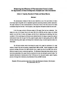
Our data come from the NBER U.S. Patent Citations Data File (Hall et al. [2001]), which has a complete record of all the citations made by patents granted between 1975 and 1999 and detailed information on all the U.S. patents granted between 1963 and 1999. Because we are ultimately interested in the market value of US businesses, we restrict our sample to include only patents that are either assigned to (i.e. owned by) domestic companies or individuals, or granted to the US inventors. Our restricted sample includes 1,222,202 patents and 7,056,477 citations. Figure 1 shows the number of patents granted by year in our sample and the share of total patents that are owned domestically. Apparently, the domestic share of US patents was steadily declining until the late 1980s and has stabilized in the 1990s at around 55 percent.Figure 2 shows the time series of the average number of citations made, for our sample, to patents within the same industry, with an industry being either a 3-digit patent class (USPTO definition) or a 2-digit patent category (Hall et al. [2001]). Note that 12 years is the maximal span of citation—lag data for patent grants in 1975. To avoid truncation bias for early years, therefore, we include only citations less than 13 years previous to the citing patent. 15
6
5
4
3
2
1
3 digit industry 2 digit industry
0 1975
1977
1979
1981
1983
1985
1987
1989
1991
1993
1995
1997
1999
Figure 2: Number of citations made to patents in the same industry, 1975-1999.
4.2
Measuring complementarity and the rate of innovation
In order to have the longest possible time series, i.e., 1975-1999, we look at backward citation lags (that is to say, lags for citations made rather than citations received). We compute citation lags by year, conditional on lags being shorter than 13 years. We restrict attention to citations made to patents that belong in the same 2 or 3—digit class – to secure as much consistency as possible with our model. Figure 3 shows the resulting conditional means for the minimum and maximum citation lags by year. Naturally, the distribution of citation lags has a wider support with 2 rather than 3-digit codes. Because the data force us to drop citation observations with lags exceeding 12 years, we first derive the conditional mean lags that the model predicts. Let Sjt denote a random variable equal to the maximum citation lag among the citations made by the most recent patent in industry j, and let sjt denote the minimum citation lag for the same patent. Then we have Proposition 4 For any λ, T > 0 and any θ ∈ (0, 1) µ ¶ 1 λT E (sjt |Djt > 0, sjt ≤ T ) = s¯ (λ, T ) = 1 − λT , (29) λ e −1 µ ¶ λT θ − 1 − λT θ λT e 1 1 − λT − . (30) E (Sjt |Djt > 0, Sjt ≤ T ) = S¯ (λ, θ, T ) = λ (1 − θ) e −1 θ (eλT − 1)
Proof: See Appendix. Our calibration procedure is as follows. Let st and St be the observed minimum and maximum citation lags in year t = {1975, ..., 1999}, and let sMA and StMA be their corresponding t T -year moving averages, with T = 13. We first determine λt by solving the equation , t = 1975, ..., 1999. s¯ (λt , T ) = sMA t
16
9 8.5 8 7.5 7 6.5 Minimum lag, 2 digit 6 Maximum lag, 2 digit 5.5
Minimum lag, 3 digit
5
Maximum lag, 3 digit
4.5 4 3.5 1975
1977
1979
1981
1983
1985
1987
1989
1991
1993
1995
1997
1999
Figure 3: Minimum and maximum backward citation lags, mean across patents by year, conditional on lag shorter than 13 years. We then compute the T -year moving average of our estimate λMA and plug it into the t equation ¡ ¢ S¯ λMA , θt , T = StMA , t = 1975, ..., 1999 t
to determine θt . Given initial condition IC, our model implies the average minimum and maximum conditional lags are constant; hence, we use moving averages to smooth short-run anomalies. Figure 4 shows two sets of estimates for θt and λt , year by year. Each set corresponds to the citation—lag data from Figure 3 that uses either the 2 or 3—digit definition of an industry. The estimated rate of innovation λt falls slightly from 0.17-0.18 to 0.145-0.16 in the late 1980s and then it rises to around 0.20 in the late 1990s. The rising and subsequently falling minimum citation lag in Figure 3 drives the time pattern of λt . Qualitatively, the latter pattern is consistent with the time series of patent grants by year in Figure 1, where patent grants fall in the 1970s and early 1980s and then rise. Our estimate of θt rises from 0.67-0.71 in 1975 to 0.82-0.85 in the early 1990s and then becomes flat right about the time when λt starts rising. The joint behavior of θt and λt implies that the number of citations that new patents make should be rising throughout the sample period. This suggests an interesting explanation of Figure 2: during the 1970s and 1980s citations per patent were rising because ideas were becoming more complementary, but afterwards citations continued rising because new ideas were arriving more frequently. In general, as the introduction to this section predicted, our calibration implies far fewer citations than observed in the data (e.g., the average number of citations per patent according to the model cannot exceed λ · T ≈ 2.2 − 2.6). The next section addresses the issue of consistency with citation counts in more detail.
17
1
0.5
Lambda, 3 digit 0.45
0.95
Lambda, 2 digit Theta, 3 digit (right scale)
0.4
0.9
Theta, 2 digit (right scale) 0.85
0.35 0.8
0.3
0.75
0.7 0.25 0.65 0.2 0.6 0.15 0.55
0.1 1975
1977
1979
1981
1983
1985
1987
1989
1991
1993
1995
1997
0.5 1999
Figure 4: Calibrated values of λt (left scale) and θt (right scale) by year.
4.3
Consistency with data on citation counts
It may seem easy to calibrate λ and θ with the available data on citations made per patent and average citation lags. These statistics (with the advantage of no truncation) are available in Hall et al. [2001]. Their counterparts can be computed in the model as well. The most recent patent in industry j makes Djt citations. The next proposition derives the expression for the mean number of citations and the mean citation lag.5 Data from Hall et al. [2001]: Mean number of citations per patent
Mean citation lag
Calculated parameters:
θ
λ
1975-1977
5
14.33
0.83
0.24
1997-1999
10
12.66
0.91
0.47
Table 1. Alternative calibration of λ and θ. Proposition 5 In the model, let Sˆjt be the average citation lag across all the citations made by the most recent patent in industry j. Then E (Djt ) =
Proof: See Appendix.
³ ´ E Sˆjt |Djt > 0 =
θ , 1−θ
µ ¶ θ 1 1− . λ (1 − θ) 2
5
(31) (32)
Our definition of mean citation lag first computes the average citation lag for an individual patent and then averages this average across patents. This is the statistic that Hall et al. [2001, p. 18] call “mean citation lag by patent”.
18
8
Raw 7
Adjusted for clustering
6
Adjusted, within 2 digit industry Adjusted, within 3 digit industry
5 4 3 2 1 0 1975
1977
1979
1981
1983
1985
1987
1989
1991
1993
1995
1997
1999
Figure 5: Raw and adjusted citations made, conditional on citation lags of 12 years or less. Table 1 uses expressions (31)-(32) to estimate λ and θ from average citations per patent and average citation lags taken from Hall et al [2001] (Sections II.6 and II.7). The estimates of θ and λ are higher than those in the previous section. The reason is the high number of citations per patent. When this number is high, (31) implies a value of θ close to 1; when θ is big, (32) requires a high value of λ to match the average citation lag. Upon closer examination of the data, it turns out that the high number of citations in Table 1 may be driven by citation clusters, that is, multiple citations that have the same lag. As we argued in the introduction to this section, citation clusters tend to arise when a single innovation is covered by multiple patents. Since the model associates each citation with a separate derivative idea, the presence of citation clusters will our estimation to overstate the number of derivative ideas. This causes the high estimates of θ in Table 1. In our sample, citation clustering is much more likely than chance would dictate. For example, among the 159,181 patents that make exactly 3 citations with lags of 12 years or less, 4,210 patents, or 2.64 percent, have all 3 citations with the same lag. This is almost more likely than ¡ 14¢times 2 the probability of this cluster occurring by chance, which equals 12 ≈ 0.007. Another potential problem with citation counts is categorizing citations made to patents outside of own industry. The model has no interpretation for these citations, since innovation processes are assumed to be industry specific. Because of this, we prefer to exclude citations made to patents outside of own industry. Figure 5 makes adjustments to raw citation counts in our data. The top line labeled “Raw” shows the number of citations made per patent, conditional on lags being 12 years or less. The “Adjusted” line replaces every citation cluster with a single citation. The raw and adjusted citation counts move apart in the 1990s, indicating that multi-patent innovations may have become more prevalent in the later years. The bottom two lines additionally remove citations made to patents outside the same industry (2 digit or 3 digit), which eliminates another 20-25 percent of citations. Table 2 re-calculates values of λ and θ using adjusted mean citations per patent. The adjustment is as follows. Figure 5 shows that raw citations should be “deflated” by a factor 19
of approximately 1.5 in 1975-1977 and a factor of 2.25 in 1997-1999 to account for citation clusters and citing outside own industry. We do not make adjustments to mean citation lags (although we think that the mean lag for 1997-1999 should probably be adjusted upwards, because clusters become more frequent during the 1990s and drag the average lag down, raising the estimate of λ). Adjusted data from Hall et al. [2001]: Adjusted number of citations per patent
Mean lag
1975-1977
3.30
1997-1999
4.43
Calculated parameters:
Calibration based on minimum and maximum citation lags
θ
λ
14.33
0.76
0.18
0.67-0.74
0.17-0.18
12.66
0.82
0.25
0.80-0.84
0.20-0.21
θ
λ
Table 2. Consistency between alternative calibrations of λ and θ. Overall, the results in Table 2 are consistent with Section 4.2. The parameter levels implied by both calibrations are close, and the rise in θ and λ is evident in all cases. The main difference from the calibrations in Section 4.2 is that the change in θ is somewhat smaller and the rise in λ is bigger. However, as stated, we believe that the fourth column of Table 2 overstates the rise in λ (because citation clusters bias the mean citation lag downwards).
5
Numerical Results
Section 4 uses U.S. patent data to find numerical estimates of λ and θ, where the former indexes the rate of innovation in the economy and the latter the degree of complementarity among new ideas. The evidence suggests that both have risen. To isolate the effects of changes in these parameters, we calibrate the remainder of the model to U.S. data prior to 1975.
5.1
Calibrating the model to the US economy
The statistics that we use for calibration are the long—run growth rate of GDP per worker, gc = 0.020; the average (1952-72) ratio of business investment to non-housing GDP, ic = 0.132; labor’s share, ζ c = 0.700; and, the average (1952-72) ratio of the market value of businesses to GDP, ω c = 1.780.6 We set conventional parameters δ = .10, n = .01, and ρ = .02. For selected values of λ and θ, together with (δ, n, ρ) = (.10, .01, .02) and (g , i , ζ , ω) = (gc , ic , ζ c , ω c ), solution of the following equations yields values for remaining parameters (η , z , α , σ) and balanced growth levels (m∗ , k∗ , r∗ ): η
m∗ =
a∗ · m− 1−η
ζ= 6
1
a∗ · m− 1−η
,
1−α , m∗
Market value of businesses is from Laitner and Stolyarov [2003].
20
(33) (34)
³ η ´1−η 1 λ z 1−η − 1 = g, η 1−α 1 ¶ 1−α µ i k∗ = , δ+n+g α α−1 k − δ, r∗ = m∗ ∗ Vt + Kt ω∗ = = (a∗ · u∗ ) + k∗1−α = ω, Yt r∗ − ρ σ= . g
(35) (36) (37) (38) (39)
Equation (33) is the expression for aggregate markup from the Corollary to Lemma 1. Equation (34) follows from Lemma 1. Equation (35) uses (16) and (13); equation (36) follows from y∗ − c∗ = i · k∗α and (17) with k˙ t = 0; (37) follows from (10); (38) follows from (28); and (39) uses (15) and the fact that along a balanced growth path C˙ t /Ct = n + g. Table 3 presents the calibrated values for η, z, α, σ, r∗ , m∗ , k∗ and v∗ =
Vt Yt · = (a∗ · u∗ ) · k∗α . 1 Yt Z 1−α L t t
The last two columns show the corresponding number of markup states and the average life span7 for a fundamental patent, S = 1/ [λ (1 − θ)]. Section 4 suggests λ ∈ [0.15, 0.20] and a 1975 value θ ∈ [0.67, 0.74].
λ
θ
0.150
0.67
0.150
η
Calibrated parameters
Steady state variables
z
α
σ
m*
r*
k*
v*
0.870
1.083
0.216
3.485
1.120
0.090
1.020
0.768
2
20.2
0.74
0.884
1.080
0.221
3.760
1.113
0.095
1.020
0.768
2
25.6
0.175
0.67
0.858
1.074
0.215
3.431
1.122
0.089
1.020
0.768
3
17.3
0.175
0.74
0.877
1.072
0.220
3.694
1.115
0.094
1.020
0.768
3
22.0
0.200
0.67
0.841
1.068
0.214
3.404
1.122
0.088
1.020
0.768
3
15.2
0.200
0.74
0.867
1.065
0.219
3.645
1.116
0.093
1.020
0.768
3
19.2
H S
Table 3. Calibration results. The calibrations always imply limit pricing; so, the economy features multiple markup states. A higher λ requires a lower η and z to match growth rate gc ; consequently, the number of markup states H rises with λ. For example, λ = 0.15 leads to markup vector m = (z, 1/η)T , and λ = 0.20 to m = (z, z 2 , 1/η)T . The calibrated η implies an elasticity of substitution for intermediate inputs of 1/(1 − η) ≈ 7. This elasticity plays an important role: the higher it is, the better the economy can reallocate resources towards sectors with the highest TFP levels, and the more the leading sectors affect aggregative TFP growth. 7
Note that our model induces a Poisson process for fundamental patents with Poisson parameter λ(1 − θ).
21
The calibrated average markup is within a narrow range around 1.12, which is consistent with empirical evidence in Jones and Williams [2000].8 The tightness of range carries over to α, σ, and the balanced growth interest rate r∗ – for which we find a value around 0.09. We select θ = 0.67 and λ = 0.175 — values corresponding to estimates of θ1975 and λ1975 in Figure 4 — as our “baseline case.” See the third row of Table 3.
5.2
Comparisons of balanced growth equilibria
We study the effects of finite changes in λ, θ, z, and ρ, and present 4 simulations. Each holds (δ, n , η, α, σ) constant at the baseline level of Table 3, row 3 – solving for the new balanced growth level of (g, i, ζ, ω, m∗ , k∗ , r∗ , v∗ , H). Table 4 presents results as changes relative to baseline.
Case 1
Case 2
Case 3
Case 4
Exogenous changes Δθ
0.15
0.15
0.15
0.15
Δλ
0
0.025
0.025
0.025
Δz
0
0
-0.008
0
Δρ
0
0
0
-0.0098
Endogenous responses Δg
0
0.0029
0
0.0029
Δr*
0
0.0098
0
0
Δm*
0.0174
0.0174
0.0119
0.0174
Δv* / v*
0.5226
0.3295
0.4224
0.468
Δ ω* / ω*
0.2185
0.1155
0.1772
0.195
Table 4. Simulation results. Case 1 We first raise θ from 0.67 to 0.82, a change consistent with the calibration in Section 4.2 that uses the 3-digit definition of an industry. Equation (35) shows the growth rate g remains the same. A higher degree of complementarity raises the average markup m∗ , however, and lengthens the average life span of fundamental patents. The long—run interest rate, pinned down by the Euler equation, remains unchanged. Hence, v∗ and the market value—to—GDP ratio ω ∗ rise. As the markup rises, labor’s share declines. The rising markup also causes the capital per effective worker, k∗ , and the investment—to—GDP ratio to decline slightly. The value of ideas (i.e., v∗ ) rises more than 50 percent, and ω ∗ rises more than 20 percent. Case 2 By the end of the sample in Section 4, λ had risen from 0.175 to 0.200; hence, our second simulation combines ∆θ = 0.15 and ∆λ = 0.025. In this case, the overall TFP growth rate increases about 0.3 percent per year. In turn, r∗ rises, with ∆r∗ = σ · ∆g. The 8
See also Basu (1993), Norrbin (1993) and Laitner and Stolyarov (2004).
22
increase in λ increases the rate of creative destruction. That, together with the increase in the interest rate, lowers the degree to which the value of fundamental ideas increases. The increase in v∗ is 33 percent in case 2 as opposed to 52 percent in case 1. Case 3 Assuming there is insufficient evidence to conclude that TFP growth permanently increased in the 1990s, the third simulation carries over the increases in θ and λ from the second but offsets the increase in λ with a sufficient decrease in technology step size z to hold the growth rate g constant. In other words, the quantity of innovations increases but the quality declines. This might, in fact, be a description of a consequence of changes in U.S. patent policy in the 1980s that strengthened patent protection and broadened patent scope. Hunt [2001, p.12] and Jaffe and Lerner [2004, ch.1-2], for instance, suggest that patent policy changes may have led to a decline in patent quality. Table 4 shows that in the third simulation, the average markup is higher than its baseline level, since complementarity is higher. However, m∗ is lower than in cases 1-2 because the step size for limit pricing depends on z, which is now lower. This tends to decrease the value of patent pools over cases 1-2. On the other hand, since overall growth is slower in case 3 than 2, the interest rate does not increase. On balance, the third simulation’s lower average markup reduces the increase in intangible wealth, v∗ , to 42 percent rather than the 52 percent of case 1, but the interest rate effect makes the second simulation’s increase in v∗ , 33 percent, the lowest of cases 1-3. Case 4 The fourth simulation repeats the changes in θ and λ of cases 2-3 but adjusts the consumer’s subjective discount rate to keep r∗ constant. The value of z does not change from the baseline. As one might expect, the increase in the value of intangible wealth is greater than simulation 2, where the interest rate rose, and greater than simulation 3, where patent quality, hence the average markup, fell. The percentage rise in v∗ is about 47 percent – almost as high as case 1, where the rate of creative destruction did not increase. (Although the change in ρ is artificial in the sense of being contrived for the sake of studying the role of the interest rate, conceivably a constant interest rate could emerge in practice in a model with open—economy international financial capital flows.) Robustness Other calibrations of θ suggest a somewhat smaller percentage change in the complementarity parameter than our baseline simulation. For example, the calibration based on a 2-digit definition of industry has ∆θ/θ ≈ 0.2 and the alternative calibration in section 4.3 has ∆θ/θ ≈ 0.08. We calculate the elasticities of v∗ , ω ∗ and r∗ with respect to λ and θ (computed at the baseline parameter values). Write v∗ and ω∗ as v∗ = v∗ (θ, λ, r∗ (λ)) , ω∗ = ω∗ (θ, λ, r∗ (λ)) , where
³ η ´1−η 1 1−η −1 r∗ (λ) = ρ + σg = ρ + σλ z η 1−α
is the long-run interest rate (that is pinned down by the Euler equation). Taking logdeviations in the above expressions and substituting the values of elasticities (computed
23
numerically) yields ∙ ∆v∗ ¸ v∗ ∆ω ∗ ω∗
= = =
∙
∙
∙
εv,θ εω,θ 1.69 0.7 1.69 0.7
¸
¸ ∙ ∆θ ∆λ εv,λ + εv,r · εr,λ · · + = εω,λ + εω,r · εr,λ θ λ ¸ ¸ ∙ ∆θ ∆λ −0.46 + (−0.73) · 0.77 · · + = −0.20 + (−0.52) · 0.77 θ λ ∙ ¸ ¸ ∆λ ∆θ −1.02 + · . · −0.60 θ λ
(40)
A rise in θ makes the value of patents rise, because fundamental ideas live longer and have a higher probability of capturing rents from a derivative innovation. A rise in λ, by contrast, makes both v∗ and ω ∗ drop. A larger λ affects v∗ both directly, through an increase in the rate of creative destruction, and indirectly, through a higher long-run interest rate. The magnitude of the creative destruction (direct) effect of λ on v is εv,λ = −0.46. The interest rate (indirect) effect, εv,r · εr,λ = (−0.73) · 0.77 = −0.56, is somewhat larger. Thus smaller changes in θ will make v∗ and ω ∗ rise by less, and (40) shows by how much. The same expression also shows that the direct elasticities of v∗ and ω ∗ with respect to λ, εv,λ and εω,λ , are comparatively small.
5.3
Market value of businesses
Figure 6 shows time series actual values for ω t . The level of ω t rose from a trough in the early 1980s. The rate of increase evidently became unsustainably high in the five years beginning 1995. However, there may be a linear trend from 1984, with ω 1984 ≈ 1.55, to the early 2000s, which levels off at a plateau of ωt = 2.55. The trough—to—peak percentage increase would be 45-50. Table 4 produces increases in ω ∗ never exceeding half of that. Other papers provide alternative explanations — for example, changes in tax rates on capital (McGrattan and Prescott [2005]). Nevertheless, the patent data may suggest an interesting possibility for part of the rise. Consider simulation 3 more closely. The overall rate of TFP growth never changes. Section 4 suggests that θ rose from 1975 to 1992. As stated above, this could have followed from changes in patent policy (i.e., more generous treatment of patent rights). With higher markups and longer life spans for fundamental patents, perhaps the stock market bid up the value of intangible capital. Section 4 shows that λ subsequently rose fairly strongly. Indeed, a surge in patent grants is evident in Figure 2 (starting in the 1980s, but gathering force in the 1990s). Perhaps the change in patent policy – and the stock market run-up that ensued – attracted more patent applications. It even seems possible that financiers’ miscalculations on the extent to which competition among patents would increase the rate of creative destruction contributed to the spike, and backtracking, in Figure 6 in the late 1990s.
6
Conclusion
This paper expands a neoclassical model based on quality ladders to include complementarities between sequential innovations. By distinguishing “fundamental” from “derivative” (i.e., “application”) inventions and incorporating both, it combines recent microeconomic concerns with interdependencies and spillovers with macroeconomic analyses of general equilibrium 24
3.60
3.10
2.60
2.10
1.60
1.10
0.60 1952
1957
1962
1967
1972
1977
1982
1987
1992
1997
2002
Figure 6: Market value of businesses to GDP ratio, 1952-2006. Data source: Flow of Funds, NIPA. growth. The scope of the model is enhanced — the separate natures of fundamental and derivative innovations seem important in practice as well as in existing literatures — yet we are able to derive an aggregate production function with a quite straightforward structure. What is more, the new analytical framework provides us with a template for utilizing potentially rich, but otherwise difficult to interpret, U.S. patent data. After generalizing the neoclassical framework to encompass technological complementarities, we show that the new model puts U.S. patent data into a more useful perspective — enabling us to use several elements of it for calibration. In fact, the scope of the calibration exceeds the number of parameters new to the model. The quality ladder model presents technological progress, roughly speaking, as the product of the frequency of innovation, λ above, and average quality per innovation, z above. The decomposition has potentially great interest, because λ and z may change over time, and affect the macroeconomic variables in ways different from the change in the rate of progress alone. For example, the economy’s intangible wealth is, roughly speaking, dependent on z/λ (i.e., the product of the price markup and the average duration of a patent). Using our enhanced model, we can employ data on patent citations and citation lags to calibrate not only a new parameter measuring the average degree of complementarity among patents — which is of interest itself — but also λ. Sections 4-5 provide calibrations based on data from 1975-99. The degree of complementarity has increased over this period, and we suggest that changes in patent policy may be at least part of the reason. In turn, the model implies that rising complementarity has exerted upward pressure on the market value of intangible wealth (i.e., knowledge capital). This may have been a contributing factor to the run up of the U.S. stockmarket in the period after 1980.
25
References [1] Barbarino, Alessandro Jovanovic, Boyan “Shakeouts and Market Crashes”, NBER Working Paper No. w10556 (June 2004). [2] Barro, Robert J., Sala-i-Martin, Xavier, “Economic Growth”Cambridge, Mass.: MIT Press, 1999. [3] Basu, Susanto. “Procyclical Productivity: Overhead Inputs or Cyclical Utilization?”, The University of Michigan, mimeo 1993. [4] Belenzon, Sharon; “Knowledge Flow and Sequential Innovation: Implications for Technology Diffusion, R&D and Market Value”, University of Oxford Deparetment of Economics Discussion Paper series, No 259, March 2006. [5] Bessen, James; Maskin, Eric, (2006) “Sequential Innovation, Patents, and Imitation” Institute for Advanced Study, School of Social Science, Economics Working Papers: 0025, 2006. [6] Caballero, R. J. & Jaffe, A. B. (2002). “How high are the giants’ shoulders: An empirical assessment of knowledge spillovers and creative destruction in a model of economic growth”. In A. B. Jaffe & M. Trajtenberg (Eds.), Patents, Citations and Innovations: A Window into the Knowledge Economy. Cambridge: MIT Press. [7] Chang, Howard F., “Patent Scope, Antitrust Policy, and Cumulative Innovation,” The Rand Journal of Economics 26, no. 1 (Spring 1995): 34-57. [8] Chu, Angus, (2007) “Effects of Blocking Patents on R&D: A Quantitative DGE Analysis”, working paper, Institue of Economics, Academia Sinica. [9] Hall, B. H., Jaffe A.B. and Trajtenberg M. (2001). “The NBER patent citations data file: Lessons, insights, and methodological tools”. NBER Working Paper No. w8498 (October 2001) [10] Hall, B. H., Jaffe A.B. and Trajtenberg M. (2005), “Market Value and Patent Citations”, RAND Journal of Economics, Vol. 36(1), pp. 16-38. [11] Hogg, R.V., and Craig, A.T., Introduction to Mathematical Statistics. 5th edition.Upper Saddle River, NJ: Prentice Hall, 1995. [12] Howitt, Peter. “Measurement, Obsolescence, and General Purpose Technologies.” In General Purpose Technologies and Economic Growth, Elhanan Helpman (Ed). Cambridge, MA: MIT Press, 1998, 219-51. [13] Griliches, Zvi, “Patent Statistics as Economic Indicators: A Survey,” Journal of Economic Literature 28, no. 4 (Dec 1990), pp. 1661-1707. [14] Green, Jerry R.; Suzanne Scotchmer “On the Division of Profit in Sequential Innovation”, The RAND Journal of Economics, Vol. 26, No. 1. (Spring, 1995), pp. 20-33. [15] Grossman, Gene M., Elhanan Helpman, “Quality Ladders in the Theory of Growth”, Review of Economic Studies, Vol. 58, No. 1. (Jan., 1991), pp. 43-61. [16] Hunt, Robert M., “You can patent that? Are patents on computer programs and business methods good for the new economy?” Federal Reserve Bank of Philadelphia Business Review Q1 2001, pp. 5-15.
26
[17] Jaffe, Adam B. and Josh Lerner, “Innovation and its discontents : how our broken patent system is endangering innovation and progress, and what to do about it”, Princeton, NJ: Princeton University Press, 2004. [18] Jones, Charles I.; Williams, John C., ”Too Much of a Good Thing? The Economics of Investment in R&D”, Journal of Economic Growth v5, n1 (March 2000): 65-85. [19] Kortum, Samuel, “Research, Patenting and Technological Change”, Econometrica v65 n6 (November 1997): 1389-1419. [20] Kortum, Samuel and Josh Lerner, “What is behind the recent surge in patenting?”, Research Policy, Volume 28, Issue 1 (January 1999): 1-22. [21] Laitner, John P., Stolyarov, Dmitriy, “Technological Change and the Stock Market”, American Economic Review, vol. 93, no. 4 (Sep 2003): 1240-67. [22] Laitner, John P., Stolyarov, Dmitriy, “Aggregate Returns to Scale and Embodied Technical Change: Theory and Measurement”, Journal of Monetary Economics, vol. 51, no 1 (Jan 2004): 191-233. [23] Levin, Richard C; Alvin K Klevorick; Richard R Nelson; Signey G Winter; Richard Gilbert; and Zvi Griliches. “Appropriating the Returns from Industrial Research and Development,” Brookings Papers on Economic Activity 1987, no. 3, Special Issue on Microeconomics. (1987), 783-831. [24] Matutes, Carmen; Regibeau Pierre and Katharine Rockett, 1996. “Optimal Patent Design and the Diffusion of Innovations,” RAND Journal of Economics, vol. 27(1): 60-83. [25] McGrattan, Ellen R.; Edward C. Prescott (2005) “Taxes, Regulations, and the Value of U.S. and U.K. Corporations” Review of Economic Studies 72 (3), 767—796. [26] Norrbin, Stefan “The Relationship Between Price and Marginal Cost in US. Industry: A Contradiction,” Journal of Political Economy (December 1993), 1149—1164. [27] O’Donoghue, Ted, Zweimuller, Joseph, “Patents in a Model of Endogenous Growth”, Journal of Economic Growth, vol. 9, no. 1 (March 2004): 81-123. [28] Pastor, Lubos, and Veronesi, Pietro, “Technological Revolutions and Stock Prices”, CEPR Discussion Papers: 5428; London: Centre for Economic Policy Research, 2006. [29] Schmookler, Jacob, Invention and economic growth, Cambridge : Harvard University Press, 1966. [30] Scotchmer, Suzanne, “Standing on the Shoulders of Giants: Cumulative Research and the Patent Law,” The Journal of Economic Perspectives 5, no. 1 (Winter 1991): 29-41. [31] Scotchmer Suzanne, “Protecting Early Innovators: Should Second-Generation Products be Patentable?”, The Rand Journal of Economics 27, Summer 1996, 322-331. [32] Segerstrom, Paul S., “Innovation, Imitation, and Economic Growth” The Journal of Political Economy, Vol. 99, No. 4. (Aug., 1991): 807-827. [33] Trajtenberg, Manuel (2002) “A Penny for Your Quotes: Patent Citations and the Value of Innovations.” In A. B. Jaffe & M. Trajtenberg (Eds.), Patents, Citations and Innovations: A Window into the Knowledge Economy. Cambridge: MIT Press. 27
[34] Trajtenberg, Manuel, Rebecca Henderson, and Adam B Jaffe. (2002) “University versus Corporate Patents: A Window on the Basicness of Invention.” In A. B. Jaffe & M. Trajtenberg (Eds.), Patents, Citations and Innovations: A Window into the Knowledge Economy. Cambridge: MIT Press. [35] Van Mieghem, Jan A. Performance Analysis of Communications Networks and Systems, Cambridge University Press, 2006
28
Appendix: Proofs Proof of Lemma 1: For more compact notation, omit the time subscript throughout the proof. Using industry production function (3), the demands for capital and labor are R=α
xj xj , W = (1 − α) . Kj Lj
(41)
Then every industry must have the same capital-labor ratio k = Kj /Lj = K/L. Let lj = Lj /L denote the fraction of the total labor force employed in industry j. The demand curve for industry j implies 1 1 1 1 Y = [pj ] 1−η = [mj ] 1−η c 1−η [Zj ]− 1−η xj 1
1
1
1
1
η
⇐⇒ Y = xj [mj ] 1−η c 1−η [Zj ]− 1−η = kα L · lj · [mj ] 1−η c 1−η [Zj ]− 1−η
η 1 1 Y − 1−η − 1−η 1−η . [m ] c [Z ] j j K α L1−α Then, plugging (42) into the labor market clearing condition, Z 1 Z 1 η 1 Y lj dj = [mj ]− 1−η [Zj ] 1−η dj 1= 1 0 K α L1−α c 1−η 0
⇐⇒ lj =
(42)
1
Y c 1−η ⇐⇒ Z = α 1−α = R 1 . η 1 − 1−η K L 1−η dj [m ] [Z ] j j 0
To get c as a function of Zj and mj , use (1): Y =
µZ
1
xηj dj
0
¶ η1
=
µZ
1 α
η
(Zj k lj L) dj
0
¶ η1
=
µZ 1 ³ ´η ¶ η1 1 1 1 =Y from (42) [mj ]− 1−η c− 1−η [Zj ] 1−η dj 0
⇐⇒ c
1 1−η
This proves (7). From (41),
=
µZ
1
[Zj ]
η 1−η
η − 1−η
[mj ]
0
dj
¶1/η
RK = αX and W L = (1 − α) X, where X = Substituting these into (4) yields ¶1−α µ ¶α µ W X R = α 1−α . c= α 1−α K L Define m=
Z
1
lj mj dj.
0
29
.
Z
0
(43)
1
xj dj.
(44)
Zero profit in the final goods sector implies Z 1 Z 1 c Y = pj xj dj = mj Zj lj kα Ldj = cmK α L1−α 0 0 Zj
(45)
⇐⇒ Y = mX. Substituting X = Y /m into (44) proves the first two conditions in (8). The third one follows from accounting. It is left to prove (9). Expressions (45) and (6) imply m=
Z , c
(46)
and substituting from (7) and (43) into (46) completes the proof. Proof of Corollary to Lemma 1: If the initial distribution of markup states is a∗ , the markup state of an industry is independent of its number of arrivals Njt . That is, for any j, Zjt and mjt are independent, with mjt being a realization of a random variable m ˜ distributed according to (m, a∗ ), and Zjt being a realization of a random variable Z˜t = Z0 · z Nt , where Z0 has some distribution with a finite mean and Nt has a Poisson distribution with parameter λt. We can use the law of large numbers (for a sample indexed by j) and the independence of Z0 , Nt and m ˜ to compute the integrals in (9) and (7) as follows: ∙h i η ¸ η 1−η − R1 η η E Z˜t [m] ˜ 1−η [Zjt ] 1−η [mjt ]− 1−η dj 0 ¸= = ∙h i η mt = R 1 η − 1 1 1−η 1−η [m ] 1−η dj − [Z ] jt jt 0 E Z˜t [m] ˜ 1−η
Similarly,
∙h i η ¸ h i η 1−η η · E [m] ˜ − 1−η E Z˜t a∗ · m− 1−η ∙h i η ¸ 1 . h i= − 1−η 1 1−η − 1−η a · m ˜ ∗ · E [m] ˜ E Zt
µ ∙h i η ¸¶1/η i´1/η ³ h η i´1/η ³ h η i´1/η ³ h η 1−η − η Nt − 1−η 1−η E Z˜t [m] ˜ 1−η 1−η · E z · E m ˜ E Z0 ¸ ∙h i η = Z (t) = = h η i h i h η i 1 1 N − 1−η 1−η 1−η − 1−η 1−η t ˜ · E z · E m ˜ E Z E Zt [m] ˜ 0 ³ h i´1/η η − 1−η 1−η i´ ³ h η i´ 1−η ³ h E m ˜ η η η i . h = E Z01−η · E z 1−η Nt · 1 E m ˜ − 1−η 30
The first term of the above expression is Z¯0 , the second term equals ³ h η i´ E z 1−η Nt
1−η η
and the third term is m0 .
⎡
´N ⎤ 1−η ³ η η ¶ µ 1−η λz t ⎥ 1−η ⎢ −λt t = ⎣e = exp γ ⎦ N! η N=0 ∞ X
Proof of Proposition 1 This is a special case of Proposition 2 for H = 1 and m∗ = 1/η. Proof of Lemma 2: First, establish (22). The profit of the industry leader equals ¶ µ xjt ct xjt = (mjt − 1) ct = (mjt − 1) ct ktα Lt · ljt π jt = pjt − Zjt Zjt 1 η 1 − 1−η Yt − 1−η 1−η from (42) [m ] c [Z ] jt jt t Ktα L1−α t η η µ ¶ 1−η ¶ µ ¶ 1−η µ η η 1 − 1−η − 1−η Zjt Zjt 1−η Yt · mt = mjt − mjt from (46). Zt Zt
= (mjt − 1) ct Ktα L1−α t mjt − 1 = Yt mjt
µ
mt mjt
Next, substitute
η ¶ 1−η
Zjt = Zj0 eNjt , mt = m∗ and
h η i η η 1−η Zt1−η = E Zj0 m01−η eγt
from the Corollary to Lemma 1 into the expression for πjt and take the conditional expectation: ¶ η µ h η i η 1 η − 1−η − 1−η − η 1−η m∗1−η · Yt · Zt 1−η · E Zj0 − mh πt (h, N) = mh z N 1−η = η ¶ µ ¶ 1−η µ η 1 η − 1−η − 1−η m∗ · − mh · Yt · e−γt · z N 1−η from (11)-(13) = mh m0
−
= This proves (22). From (22),
η
−
1
mh 1−η − mh 1−η η − 1−η
a∗ · m
η
· Yt · e−γt · z N 1−η .
η
π t (h, N) = π t (h, 0) · z N 1−η , for all (h, N) . Then induction on h in (21) shows that η
vt (h, N) = vt (h, 0) · z N 1−η for all (h, N) . Finally, setting N = 0 in (21) and differentiating with respect to t proves (24). Proof of Proposition 2: First, show that H X h=1
a∗h · π t (h, 0) = Πt · e−γt . 31
Using (22) in Lemma 2, we can write H X h=1
−γt
a∗h · π t (h, 0) = (a∗ · μ) · Yt · e
¶ µ 1 · Yt · e−γt = Πt · e−γt . = 1− m∗
Next, differentiate the expression (25) for aggregate patent value and use (24) from Lemma 2 and (25) to write V˙ t = γVt + eγt
H X h=1
a∗h · v˙ t (h, 0) = (γ + λ + rt ) Vt − Πt − θλz
(γ + rt ) Vt − Πt +
Ã
λ − θλz
η 1−η
η 1−η
·e
PH
Proof of Proposition 3: Let
γt
H X h=1
h=1 a∗h · vt (h ⊕ 1, 0) P H h=1 a∗h · vt (h, 0)
a∗h · vt (h ⊕ 1, 0) =
!
Vt .
xt (h, N) = E (xjt |hjt = h, Njt = N) . Using the definition of qt (h, N), we can write qt (h + 1, N) − 1 vt (h + 1, N) = qt (h, N) − 1 vt (h, N) vt (h + 1, N) = vt (h, N)
kt (h, N) kt (h + 1, N) xt (h, N) · [from (41)] xt (h + 1, N) ¶ 1 µ mh+1 1−η vt (h + 1, N) · . [from (2)] = vt (h, N) mh ·
The fact that π t (h + 1, N) > π t (h, N) and the value equations (21) imply that vt (h + 1, N) > vt (h, N) for all N, t ≥ 0. Since mh+1 > mh , the ratio in the above expression is always strictly greater than one. Proof of Corollary to Proposition 3: Fix any t ≥ 0. Let the average value of a fundamental patent with h citations be b(h) ≡ EN [vt (h + 1, N)]. A “thread” is an active fundamental patent and all of its derivatives. Think of the class of patents at time t having h citations. One type of thread in this class has length h + 1 and consists of a fundamental patent that receives h citations. For each such thread, we can find θ other industries with thread length 2 + h and the first derivative patent in each having h citations; ... ; θ other industries with thread length 1 + + h and the ’th derivative patent in each having h citations; .... This exhausts all threads in the class. So, the class has a ratio of fundamental patents to total members of 1 = 1 − θ. θ 1 + 1−θ Hence, the average value of any patent (derivative of fundamental) that has h citations is b(h) (1 − θ). The cross-sectional covariance of patent values and citations is then ∞ X h=1
¡ ¢ (1 − θ) θh−1 b (h) (1 − θ) − ¯b · h, 32
where ¯b =
∞ X h=1
(1 − θ) θh−1 · b (h) (1 − θ) .
Proposition 3 establishes that b (·) is increasing. Thus, there is an h∗ such that b (h) (1 − θ) − ¯b ≥ 0 iff h ≥ h∗ . Then
∞ X h=1
h∗ ·
hX ∗ −1 h=1
¡ ¢ (1 − θ) θh−1 b (h) (1 − θ) − ¯b · h ≥
∞ X ¡ ¢ ¡ ¢ (1 − θ) θh−1 b (h) (1 − θ) − ¯b + h∗ · (1 − θ) θh−1 b (h) (1 − θ) − ¯b = h=h∗
¡ ¢ = h∗ ¯b − ¯b = 0
Proof of Proposition 4: The proof will use the following two facts: Fact 1. Conditional on n Poisson events within the last T periods, the joint distribution of the arrival times t1 < ... < tn is uniform on [0, T ] (Van Mieghem, 2006, p. 126). In other words, conditional on exactly n Poisson arrivals, arrival times are distributed in the same way as the set of n order statistics for the uniform distribution U [0, T ]. The marginal distribution for each th is a beta distribution with parameters h and n − h + 1 (Hogg and Craig [1995], p. 201), and its mean is Eth =
h T n+1
(47)
Fact 2. ΣN ,
N X h=0
hθh =
¡ ¢ N + 1 N+1 θ N +1 θ , for all N ≥ 0 1 − θ − 1−θ (1 − θ)2
Consider all industries where the active patent makes at least one citation. This set consists of industries where the current patent is a derivative idea and that have experienced at P∞least one Poisson event within the last T periods. The measure of such industries is n=1 θPn . An active patent in an industry that experienced n prior arrivals can make between 1 and n citations. When a patent makes h ≥ 1 citations, (47) implies that the corresponding average minimum citation lag is s (n) =
T , n+1
and the average maximum citation lag is Sh (n) =
hT . n+1
Compute the average maximum citation lag first. The probability to make h citations conditional on making at least one equals ½ P (h ∩ h ≥ 1) (1 − θ) θh−1 1 ≤ h ≤ n − 1 . = P (h|h ≥ 1) = θn−1 h=n P (h ≥ 1) 33
The mean maximum citation lag in an industry with n arrivals is ! ! Ã n−1 Ã n−2 X X T T hθh−1 (1 − θ) + nθn−1 = (h + 1) θh (1 − θ) + nθn−1 = E (Sh (n) |n) = n + 1 h=1 n + 1 h=0 ! Ã n−2 X T θh + nθn−1 = = (1 − θ) Σn−2 + (1 − θ) n+1 h=0 ¶ µ ¡ ¢ ¢ T θ ¡ n−1 n−1 n−1 n−1 = + 1−θ = 1−θ − (n − 1) θ + nθ n+1 1−θ µ ¶ T 1 θn = − n+1 1−θ 1−θ
The mean maximum citation lag across industries that experience current arrivals and make at least one citation equals P∞ θPn · E (Sh (n) |n) ¯ S = n=1 P∞ n=1 θPn To compute the numerator of this ratio, we need to evaluate two sums:
∞ ∞ ∞ X ¢ Pn 1 −λT X (λT )n+1 1 −λT X (λT )n 1 −λT ¡ λT = e = e = e e − 1 − λT , n+1 λT (n + 1)! λT n! λT n=1 n=1 n=2
and ∞ ∞ ∞ X ¢ Pn θn 1 −λT X (λT θ)n+1 1 −λT X (λT θ)n 1 −λT ¡ λT θ = e = e = e − 1 − λT θ . e n+1 λT θ (n + 1)! λT θ n! λT θ n=1 n=1 n=2
Using these expressions, the mean maximum citation lag is P∞ Pn P∞ Pn θn T T n=1 n+1 − (1−θ) n=1 n+1 1−θ = S¯ = 1 − P0 ¢ ¢ ¡ λT ¡ λT θ 1 1 − 1 − λT − − 1 − λT θ e e λ(1−θ) λθ(1−θ) = = e−λT 1 − P0 µ ¶ 1 λT eλT θ − 1 − λT θ = 1 − λT − λ (1 − θ) e −1 θ (eλT − 1)
Similarly, the mean minimum citation lag is9 : P∞ µ ¶ ∞ θPn s (n) 1 λT 1 X Pn n=1 = 1 − λT = s¯ = P∞ 1 − P0 n=1 n + 1 λ e −1 n=1 θPn 9
Note that
lim S¯ = s¯
θ→0
and
∙ ¸ 1 1 ∂ eλT θ − 1 − λT θ ¯ = T − s¯. lim S = θ→1 λ eλT − 1 ∂θ θ θ=1
34
Proof of Proposition 5: For all h ≥ 0, the probability that a patent makes h citations is θh (1 − θ). Then the mean number of citations is E (Cjt ) =
∞ X h=0
h · θh (1 − θ) =
θ 1−θ
Consider a patent that makes h ≥ 1 citations. The interval between any two consecutive innovations is λ1 . Then a patent that makes h citations has a mean citation lag of h ³ ´ 1Xi h+1 ˆ ¯ E Sjt |Cjt = h = S (h) = = . h i=1 λ 2λ
Consequently, the mean citation lag across all patents that make more than one citation is µ ¶ µ ¶ ∞ ∞ ³ ´ X X 1 h + 2 θ 1 h−1 h E Sˆjt |Cjt ≥ 1 = θ (1 − θ) = 1− . (1 − θ) = S¯ (h) θ λ 2 λ (1 − θ) 2 h=1 h=0
35