on igati & Dr Irr
ngineering sE
age System ain
Irrigation & Drainage Systems Engineering
Sando et al., Irrigat Drainage Sys Eng 2017, 6:2 DOI: 10.4172/2168-9768.1000188
ISSN: 2168-9768
Research Article
OMICS International
Using Remote Sensing to Characterize and Compare Evapotranspiration from Different Irrigation Regimes in the Smith River Watershed of Central Montana Roy Sando1, Rodney R. Caldwell1 and Kyle W. Blasch2 1 2
U.S. Geological Survey, Wyoming-Montana Water Science Center, Helena, Montana, USA U.S. Geological Survey, Idaho Water Science Center, Boise, Idaho, USA
Abstract According to the 2005 U.S. Geological Survey national water use compilation, irrigation is the second largest use of fresh water in the United States, accounting for 37%, or 484.48 million cubic meters per day, of total freshwater withdrawal. Accurately estimating the amount of water withdrawals and actual consumptive water use (the difference between water withdrawals and return flow) for irrigation at a regional scale is difficult. Remote sensing methods make it possible to compare actual ET (ETa) rates, which can serve as a proxy for consumptive water use, from different irrigation regimes at a regional scale in a systematic manner. This study investigates crucial components of water use from irrigation such as the difference of ETa rates from flood- and sprinkler-irrigated fields, spatial variability of ETa within a watershed, and the effect of sprinkler irrigation on the water budget of the study area. The mean accumulated ETa depth for the 1,051-square-kilometer study area within the upper Smith River watershed was about 467 mm 30-meter per pixel for the 2007 growing season (April through mid-October). The total accumulated volume of ETa for the study area was about 474.705 million cubic meters. The mean accumulated ETa depth from sprinkler-irrigated land was about 687 mm and from flood-irrigated land was about 621 mm from flood-irrigated land. On average, the ETa rate from sprinkler-irrigated fields was 0.25 mm per day higher than flood-irrigated fields over the growing season. Spatial analysis showed that ETa rates within individual fields of a single crop type that are irrigated with a single method (sprinkler or flood) can vary up to about 8 mm per day. It was estimated that the amount of sprinkler irrigation in 2007 accounted for approximately 3% of the total volume of ETa in the study area. When compared to non-irrigated dryland, sprinkler irrigation increases ETa by about 59 to 82% per unit area.
Introduction According to the 2005 U.S. Geological Survey national water use compilation, irrigation is the second largest use of fresh water in the United States, accounting for 37%, or 484.48 million cubic meters per day, of total freshwater withdrawals [1]. Water withdrawal for irrigation in the western United States (all states west of, and including, North Dakota, South Dakota, Nebraska, Kansas, Oklahoma, and Texas) accounted for about 85% of total irrigation withdrawals in the United States in 2005 [1]. Given the substantial quantity of water used for irrigation, numerous hydrologic investigations have studied various aspects of water withdrawals [2,1], conveyance [3], application [4], consumptive use [5,6], and return flows [7] during the irrigation process. From field-scale to national-scale assessments of irrigation water use, the wide range and accuracy of crop acreages, specific crop water-consumption coefficients, and irrigation-system application rates has created uncertainty when comparing these studies or assembling them into a national compilation. The use of remotely-sensed data, specifically satellite imagery, might be a potentially more accurate, defensible, and consistent method to estimate irrigated acreage and consumptive use, which could result in more efficient, systematic, and extensive water use estimates in agricultural settings [8-10]. Accurately estimating the amount of water withdrawals and actual consumptive use (the difference between water withdrawals and return flow) for irrigation at a regional scale is difficult. Inferring consumptive use by calculating the amount of water expelled through evapotranspiration (ET) has been a common approach. At the fieldscale, agricultural ETa has traditionally been estimated using a reference ET (ETr) value and multiplying that by crop coefficient (Kc) curves [11]. The basic procedure for estimating ETa using the crop coefficients is described by Allen and others [12]. As Allen and others suggests, for most hydrologic water balance purposes, average crop coefficients are more conveniently applied than more complex strategies that consider the temporal or spatial Irrigat Drainage Sys Eng, an open access journal ISSN: 2168-9768
heterogeneity of Kc over a growing season. However, there can be substantial within-field variation. In the last couple of decades there has been a push to differentiate the spatial and temporal heterogeneities in consumptive use using remote sensing because of its ability to provide Kc grids at various spatial and temporal scales. The idea of using remote sensing to target components of the surface energy balance and water fluxes has been around for decades [13]. With the recognition that surface temperature could be used as a proxy for estimating evaporation from wet and drying soils, Idso and others [13] determined that actual evaporation rates could be estimated from remotely acquired surface temperatures coupled with commonlycollected weather data. The method is based on the assumption that the vertical near-surface-to-air difference is an appropriate estimate of sensible heat flux and is linearly proportional to surface temperature. In other words, all other things being equal, the higher the ETa rate the colder the surrounding air temperature. Successive studies have focused on surface energy balance methods to estimate ETa from satellite imagery using different platforms and various scales [14-18,10]. Remote sensing methods make it possible to compare actual *Corresponding author: Roy Sando, U.S. Geological Survey, Wyoming-Montana Water Science Center 3162 Bozeman Ave, Helena, Montana 59601, USA, Tel: +14064575953; E-mail:
[email protected] Received August 08, 2017; Accepted August 24, 2017; Published September 03, 2017 Citation: Sando R, Caldwell RR, Blasch KW (2017) Using Remote Sensing to Characterize and Compare Evapotranspiration from Different Irrigation Regimes in the Smith River Watershed of Central Montana. Irrigat Drainage Sys Eng 6: 188. doi: 10.4172/2168-9768.1000188 Copyright: © 2017 Sando R, et al. This is an open-access article distributed under the terms of the Creative Commons Attribution License, which permits unrestricted use, distribution, and reproduction in any medium, provided the original author and source are credited.
Volume 6 • Issue 2 • 1000188
Citation: Sando R, Caldwell RR, Blasch KW (2017) Using Remote Sensing to Characterize and Compare Evapotranspiration from Different Irrigation Regimes in the Smith River Watershed of Central Montana. Irrigat Drainage Sys Eng 6: 188. doi: 10.4172/2168-9768.1000188
Page 2 of 10
ET (ETa) rates and water use from different irrigation regimes at a regional scale in a systematic manner. This study investigates crucial components of water use from irrigation such the difference of ETa rates from flood- and sprinkler-irrigated fields, spatial variability of water use within a watershed, and the effect of sprinkler irrigation on the water budget of the study area. The primary objectives of this study were to use daily reference ET (ETr) data, available from a local agricultural weather station, coupled with surface temperatures recorded by the Landsat 5 and 7 satellites to (1) provide estimates of ETa within an agricultural setting, (2) compare differences in seasonal ETa among flood and sprinkler irrigation practices without the need to adjust for crop type, (3) provide estimates of the spatial variability of ETa within individual agricultural fields for flood and sprinkler irrigation methods, and (4) estimate the effect of
current irrigation practices on the total consumptive water-use for a watershed in central Montana.
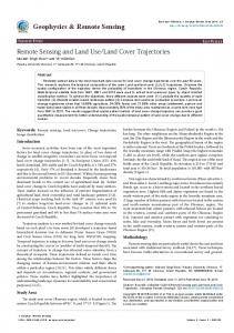
Description of study area The study area is located within the Smith River watershed in central Montana. The Smith River watershed consists of about 5,180 square kilometers (km2) of the upper Missouri River Basin in Meagher and Cascade counties of central Montana (Figure 1). The climate in the Smith River watershed is generally semiarid with some semi-humid areas in the upper elevations. Average annual precipitation (19712000) ranges from less than about 305 millimeters (mm) per year in the lowlands to over 1,000 mm per year in the surrounding mountains [19]. In 2000, water used to irrigate about 132 km2 of agricultural lands
Figure 1: Location of the Smith River watershed and study area. The study area, shaded gray, consists of the Smith River watershed upstream of Sheep Creek and is below the land surface elevation of 1,676 meters, or 5,500 feet.
Irrigat Drainage Sys Eng, an open access journal ISSN: 2168-9768
Volume 6 • Issue 2 • 1000188
Citation: Sando R, Caldwell RR, Blasch KW (2017) Using Remote Sensing to Characterize and Compare Evapotranspiration from Different Irrigation Regimes in the Smith River Watershed of Central Montana. Irrigat Drainage Sys Eng 6: 188. doi: 10.4172/2168-9768.1000188
Page 3 of 10
in the Smith River watershed accounted for about 845,000 cubic meters per day (m3/day) of water withdrawals [20]. Of the withdrawals for irrigation, surface water accounted for about 835,000 m3/day and groundwater accounted for about 10,000 m3/day [20]. About 54% of irrigated lands is hay (grass and alfalfa), 26% is spring and winter wheat, 18% is barley, 2% is classified as other [20,21]. This analysis focused on the portion of the watershed located upstream of Sheep Creek (Figure 1), where the majority (85%) of the irrigated lands are located. The analysis is limited to elevations below 1,676 meters (5,500 feet; North American Vertical Datum of 1988 [NAVD88]) due to complications with the methods when estimating ETa at higher elevations. This limitation had minimal effect on the evaluation of the assessment of ETa on irrigated agricultural lands since essentially all of the agricultural activity is found below 1,676 meters. The final focus area of analysis (study area) included 1,051 km2 of the Smith River watershed, of which 104 km2 was irrigated. Irrigated lands were defined for this study using the Final Land Unit (FLU) dataset [22].
Methods The primary method of analysis of remotely-sensed data for this study was based on the Simplified Surface Energy Balance (SSEB) method described in detail by Senay and others [10,23]. This method was chosen because it has been shown to be accurate and relatively simple to use with readily available Geographic Information System (GIS) software and publically available satellite data [23]. Landsat data were chosen for this analysis because they have an adequate spatial resolution (30 meters for optical, near-infrared, and mid-infrared bands and 120 meters (Landsat 5) and 60 meters (Landsat 7) for thermal bands) for field-scale analyses. Additionally, with a temporal resolution of 16 days, there were enough recording dates to capture multiple days throughout the growing season. Finally, Landsat data are available to the public at no charge and can be accessed at https://earthexplorer.usgs.gov/. Processing was conducted on Landsat 5 Thematic Mapper (TM) and Landsat 7 Enhanced Thematic Mapper Plus (ETM+) imagery at Path 39 Row 28. Scenes from seven dates in 2007 (03/12; 05/15; 06/16; 07/18; 08/19; 09/12; and 10/14) were selected to span the normal growing season. Individual scenes were selected to minimize areas obscured by clouds or snow. The growing season from 2007 was selected because of the availability of a relatively large quantity of unaffected Landsat imagery recorded over the study area. While most of the images used in the analysis did not require preprocessing beyond radiometric calibration, (the conversion of the data into radiance and reflectance values) two image dates (3/12/2007 and 6/16/2007) warranted additional work to replace problematic pixels obscured by clouds or snow. The issues, and steps taken to resolve those issues, are discussed in the following section.
Preprocessing of March 12th and June 16th scenes About 8% of the pixels in the March 12th image were adjusted due to cloud cover. Ideally, satellite data recorded before and after March 12th would be used to interpolate ETr to give an estimated ETr value for the pixels that were affected by cloud cover in the March 12th image. Because there was no image recorded before March 12th, a different approach was taken and is described in this paragraph. To estimate ETa for pixels that were affected by cloud cover, average land surface temperatures were calculated for each FLU land cover classification using the portion of the image that was unaffected by cloud cover. The
Irrigat Drainage Sys Eng, an open access journal ISSN: 2168-9768
FLU polygons located within the cloud-covered portion of the image were then converted to 30 meter by 30 meter pixels. The values for the pixels were defined as the average temperature for the appropriate land cover type. For instance, the average temperature, in kelvin (K), for pixels unaffected by cloud cover on March 12th that were defined as “fallow” was 285.49 K. Thus, all of the pixels that were defined as “fallow” in the cloud-covered portion of the image were replaced with 285.49 K. This was done for all of the pixels and the corresponding FLU land cover classifications that were affected by cloud cover in the March 12th image. In addition to the 8% affected by cloud cover, 19% of the March 12th image pixels represented areas covered by snow. To reduce the effects of snow cover in the March 12th image on causing unrealistically large ETa values from March to May, the pixels determined to represent snow cover were adjusted. These pixels were adjusted in the fractional ET (ETf) raster (described in the next section) by calculating the average difference of the May 15th and March 12th ETf values for non-snow covered pixels, and subtracting that difference from the May 15th image the March 12th for pixels that needed replacement. This technique was appropriate for pixels covered by snow because they were not generally located in agricultural fields, and thus had a more homogenous change in ETf between the two dates. It was decided that this approach was not as suitable for the cloud-covered pixels because the difference in ETf for those pixels varied depending on a number of factors (irrigation practice, crop type, elevation). About 5% of the pixels were adjusted in the June 16th image due to cloud cover. To replace the clouds in the June 16th image, a mask was created to encompass the cloud-covered portion of the image. This mask was used to clip out cloud-covered pixels from the June 16th image to form a “clipped image”. To ensure the pixels replacing the cloud-covered area covered the entire region clipped out from the original June 16th image, a 500 meter buffer was added to the mask. Using this enlarged mask, pixels were extracted from the May 15th and July 18th images and averaged to form a cloud replacement image. To correct for spatial differences in seasonal thermal inertia, the cloud replacement image was subtracted from the clipped image where they overlapped. The average difference was then added to the cloud replacement image to bring the land surface temperatures closer to what they would actually be on June 16th. The cloud replacement image was then mosaicked together with the June 16th image to form a corrected image.
Simplified Surface Energy Balance Processing All SSEB processing was conducted following the basic procedure described by Senay and others [10]. For SSEB processing, the cold pixels were selected based on their relatively high Normalized Difference Vegetation Index (NDVI) values and lowest thermal values of pixels with vegetation land cover and hot pixels had the lowest NDVI values and highest thermal values (Table 1). Pixels that represented open water surfaces and forested land were excluded from the analysis to avoid overestimating ETa. When the cold and hot pixels were identified for an image, all of the other pixels in that image were scaled from 0-1 based on their thermal value; 0 represented the hottest pixel value and 1 represented the coldest pixel value. This procedure effectively produced the ETf raster of pixels with values of 0-1, which is comparable to an instantaneous crop coefficient (Kc) raster. While the Landsat images provided the spatial discretization of relative hot and cold pixels throughout the study area, local reference ET (ETr) data calculated from local climatological parameters were needed to estimate ETa values. Daily ETr values for alfalfa were Volume 6 • Issue 2 • 1000188
Citation: Sando R, Caldwell RR, Blasch KW (2017) Using Remote Sensing to Characterize and Compare Evapotranspiration from Different Irrigation Regimes in the Smith River Watershed of Central Montana. Irrigat Drainage Sys Eng 6: 188. doi: 10.4172/2168-9768.1000188
Page 4 of 10 Date
Cold Pixel Temperature, in Kelvin
Cold Pixel NDVI, unitless
Hot Pixel Temperature, in Kelvin
Hot Pixel NDVI, unitless
Reference Evapotranspiration, in millimeters
Precipitation, in millimeters
3/12/2007
284.1
0.21
296.4
0.18
4.572
0
5/15/2007
289.7
0.72
308.4
0.15
5.842
0
6/16/2007
290.6
0.66
310.4
0.19
7.366
3.3
7/18/2007
293.3
0.78
311.1
0.25
9.144
1.8
8/19/2007
292.0
0.76
316.8
0.2
8.128
0
10/14/2007
287
0.77
322.1
0.19
2.0066
0
Table 1: Land surface temperature values and Normalized Difference Vegetation Index values for hot and cold anchor pixels, and reference evapotranspiration and precipitation from a nearby agricultural weather station for image dates.
obtained from the nearby U. S. Bureau of Reclamation agricultural weather (AgriMet; http://www.usbr.gov/pn/agrimet) station located in White Sulphur Springs, MT. The daily ETr values available from the AgriMet station, specifically the values reported for alfalfa, were assigned to the coldest pixels of the corresponding Landsat scene for that date. Using alfalfa as the ETr value is valid since the ETf value peaks at 1.0 for many crops when using alfalfa as the ETr [24]. Therefore, the seven Landsat scenes had corresponding ETa daily values based on the alfalfa ETr value from the AgriMet station. A daily record of ETa for each individual pixel within the study area was based on the daily values of ETr reported at the AgriMet station. To obtain daily estimates of ETa for the intervals between the individual image dates, ETf rasters were linearly interpolated between image dates. Each daily ETf raster was then multiplied by the ETr calculated at the AgriMet station for each corresponding day.
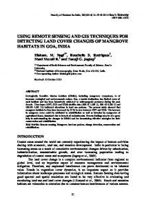
Land and vegetation categorization The land types in the Smith River watershed were designated as irrigated or non-irrigated according to the FLU dataset [22]. The FLU dataset categorized irrigation regimes based on data from 2007, which corresponded to the satellite imagery dates. Land categorized as irrigated was further subcategorized into flood, pivot (center pivot sprinkler irrigation), or sprinkler (hand line or wheel line) irrigated. For this study, all pivot and sprinkler irrigated subcategories were combined into one sprinkler irrigated subcategory (Figure 2). Floodirrigated land accounted for 4.6% (48 km2) and sprinkler irrigated-land accounted for 5.3% (56 km2) of the total study area (1,051 km2). Grassland accounts for the majority (about 77%; Table 2) of nonirrigated land cover in the study area (National Agricultural Statistics Service (NASS) Cropland Data Layer (CDL) [21]. Grassland accounts for about 67% of flood-irrigated land (Table 2) and alfalfa accounts for about 48% of sprinkler-irrigated land (Table 2).
Results and Discussion Total actual evapotranspiration The mean accumulated ETa depth for the 1051 square kilometer (km2) study area within the upper Smith River watershed was about 467 millimeters (mm) per 30m pixel. The total accumulated volume of ETa for the study area was about 474.705 million cubic meters (m3; 385,000 acre-feet) for the 2007 growing season. This includes ETa from all irrigated and non-irrigated lands, including the riparian areas along streams. For perspective, total streamflow at USGS gaging station on the Smith River near Ft. Logan, MT from March 1, 2007 to October 15, 2007 was 3.12 billion cubic meters (station number 06076690; Figure 1) (110.3 billion cubic feet) [25]. Furthermore, there was about 170 mm of precipitation in the same time period (White Sulphur Springs AgriMet; http://www.usbr.gov/pn/agrimet).
Irrigat Drainage Sys Eng, an open access journal ISSN: 2168-9768
Comparison of actual evapotranspiration rates from floodand sprinkler-irrigated crops The mean accumulated ETa depth from flood-irrigated land was about 687 mm and about 621 mm from sprinkler-irrigated land. Total accumulated volume of ETa was about 30.025 million m3 (24,341 acrefeet) for about 48.232 million square meters (m2) (11,918 acres) of flood-irrigated land and about 38.357 million m3 (31,096 acre-feet) for about 55.808 million m2 (13,790 acres) of sprinkler-irrigated land. The mean daily rates of ETa occurring in flood- and sprinklerirrigated fields showed a similar pattern from the beginning of April through the end of May. Starting in May, ETa from flood-irrigated fields begins to decrease in relation to sprinkler-irrigated fields. On average, the ETa rate from April 1st to October 14th of sprinklerirrigated fields was 0.25 mm per day higher than flood-irrigated fields. In general, ETa from flood- and sprinkler-irrigated fields in the upper Smith River watershed (Figure 2) is greatest around the middle of July with a two-week moving-average ETa rate of about 5.84 millimeters (mm) per day (Figure 3). The maximum separation of average ETa rates from the two different irrigation practices occurs in mid-August and is about 1.27 mm per day, when sprinkler is greater than flood. Total accumulated ETa from April through mid-October was about 30.025 million m3 for about 48 km2 of flood-irrigated land and 38.357 million m3 for about 56 km2 of sprinkler irrigated land. This is equal to consumptive use of about 621 mm and 687 mm for flood and sprinkler irrigated lands through the growing season, respectively. It is possible that the difference in crop types associated with different irrigation methods would affect the respective mean ETa rates; the higher % age of grassland in flood-irrigated fields and alfalfa in sprinkler-irrigated fields (Table 2) likely accounts for some of the difference in the average ETa rates.
Within-field variability Traditional ETa estimation methods that use crop coefficients are typically based on the assumption that ETa is simply a function of growing stage (estimated according to the time of the growing season) and crop type, and do not incorporate spatial heterogeneity within individual fields. The within-field ETa variability can be a consequence of a number of factors including soil conditions, field topography, plant conditions, and sprinkler positioning. It is, however, outside the scope of this study to explain the cause of such variability across and within different fields. To analyze within-field variability of ETa rates in the upper Smith River watershed 6 sprinkler-irrigated alfalfa fields and 6 flood-irrigated grass fields were chosen as a sample for the analysis. Fields were selected based on the following criteria: 1) sprinkler or flood irrigated; 2) identified as an alfalfa field (if sprinkler irrigated) or a grass field (if flood irrigated); 3) contains only pixels that were free of cloud or snow cover for image dates; and 4) fields are distributed throughout the entire study area. Fractional ET values were calculated using the
Volume 6 • Issue 2 • 1000188
Citation: Sando R, Caldwell RR, Blasch KW (2017) Using Remote Sensing to Characterize and Compare Evapotranspiration from Different Irrigation Regimes in the Smith River Watershed of Central Montana. Irrigat Drainage Sys Eng 6: 188. doi: 10.4172/2168-9768.1000188
Page 5 of 10
Figure 2: Location of flood-irrigated and sprinkler-irrigated land in the study area, upper Smith River watershed, Montana.
Irrigation Type
Miscellaneous Crops
Alfalfa
Grassland
Other
Flood Irrigated (48 km2)
2%
11%
67%
20%
Sprinkler Irrigated (56 km2)
18%
48%
29%
4%
Non-irrigated (947 km2)
0%
0%
77%
23%
Table 2: Composition of vegetative cover for flood-irrigated, sprinkler-irrigated, and non-irrigated land. Miscellaneous crops include barley, winter wheat, spring wheat, and oats. Other includes forest, shrubland, wetlands, open water, fallow fields, and developed areas.
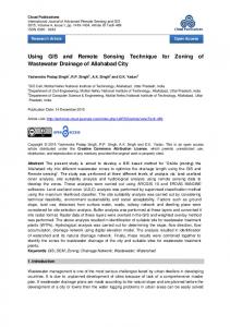
SSEB on July 18th, 2007 in a flood-irrigated field (Figure 4A) and a sprinkler-irrigated field (Figure 4B). The variability showed in Figure 4 highlights the error that can be introduced under the assumptions of a uniform crop coefficients method to estimate consumptive water-use. Results from this analysis show the highest degree of within-field variability occurred in late July and reached a single-field maximum standard deviation of about 1.78 mm per day. Mean standard deviation for all fields over the entire growing season was about 0.36 mm per day. The maximum single-field range (maximum – minimum) of daily ETa was about 7.8 mm per day and occurred in late July (fig. 5). Average Irrigat Drainage Sys Eng, an open access journal ISSN: 2168-9768
range of daily ETa for all fields over the entire growing season was about 1.9 mm per day.
Impact of sprinkler irrigation on water use Remote sensing allows for the evaluation of the net impacts or differences in mean cumulative ETa depth from different land and water-use practices. An example is an evaluation of the increase in total ETa that sprinkler irrigation has on the total accumulated ETa in the study area. As part of this exercise, all of the land area designated as sprinkler-irrigated was replaced with an average ETa depth derived Volume 6 • Issue 2 • 1000188
Citation: Sando R, Caldwell RR, Blasch KW (2017) Using Remote Sensing to Characterize and Compare Evapotranspiration from Different Irrigation Regimes in the Smith River Watershed of Central Montana. Irrigat Drainage Sys Eng 6: 188. doi: 10.4172/2168-9768.1000188
Page 6 of 10
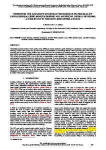
12 10 8 6 4 2 0
4/1 4/8 4/15 4/22 4/29 5/6 5/13 5/20 5/27 6/3 6/10 6/17 6/24 7/1 7/8 7/15 7/22 7/29 8/5 8/12 8/19 8/26 9/2 9/9 9/16 9/23 9/30 10/7 10/14
Average ET rate, in mm per day
14
Date of satellite image Reference ET Flood Irrigated Sprinkler Irrigated 2-week moving average of flood-irrigated 2-week moving average of sprinkler irrigated Figure 3: Comparison of average daily actual ET rates throughout the 2007 growing season calculated from flood-irrigated and sprinkler-irrigated fields in the study area. Daily reference ET values calculated at the White Sulphur Springs AgriMet (http://www.usbr.gov/pn/agrimet) and dates of satellite data collection also are shown for comparison.
Figure 4: An example of within-field variation of fractional evapotranspiration values for A) a flood-irrigated field B) a sprinkler-irrigated field on July 18, 2007 in the study area.
from non-irrigated non-riparian areas (Figure 6). To do this, all of the daily ETa rasters were summed to give an estimate of the accumulated ETa depth through the 2007 growing season. In an effort to accurately represent natural ETa from land with similar characteristics to areas that are sprinkler-irrigated, a mean cumulative ETa depth was calculated for all of the pixels that did not fall within an irrigated polygon, as defined by the FLU dataset, or within one kilometer of a stream, as defined by the National Hydrography Dataset (NHD) [26] (Figure 1). The mean
Irrigat Drainage Sys Eng, an open access journal ISSN: 2168-9768
cumulative ETa depth from those pixels, which was 432 mm, was then substituted for all of the pixels that were located within sprinklerirrigated polygons, allowing for a calculation of accumulated ETa in the study area with no sprinkler-irrigated pixels. Total accumulated ETa for the 2007 growing season across the entire study area was about 474.705 million cubic meters (m3). When the ETa attributed to sprinkler irrigation was subtracted, the total accumulated ETa was reduced to 460.525 million m3 for the study area. Volume 6 • Issue 2 • 1000188
Citation: Sando R, Caldwell RR, Blasch KW (2017) Using Remote Sensing to Characterize and Compare Evapotranspiration from Different Irrigation Regimes in the Smith River Watershed of Central Montana. Irrigat Drainage Sys Eng 6: 188. doi: 10.4172/2168-9768.1000188
9 8 7 6 5 4 3 2
9/30
9/16
10/14
Average range of ET within sprinkler irrigated fields
9/2
8/19
8/5
7/22
7/8
6/24
6/10
5/27
5/13
4/29
0
4/15
1 4/1
Range of daily ET, in millimeters per 30 meter pixel
Page 7 of 10
Minimum range of ET within sprinkler-irrigated fields Maximum range of ET within sprinkler-irrigated fields Average range of ET within flood-irrigated fields Minimum range of ET within flood-irrigated fields Maximum range of ET within flood-irrigated fields
Figure 5: Minimum, mean, and maximum range of daily actual ET rates for the 2007 growing season within 6 sprinkler-irrigated fields and 6 flood-irrigated fields located in the upper Smith River watershed, Montana.
Figure 6: A) Accumulated actual ET for the 2007 growing season in the study area B) Accumulated actual ET for the 2007 growing season with sprinklerirrigated pixels replaced.
This means that sprinkler irrigation adds an additional 14.18 million m3 of consumptive water use in an average growing season, which is about a 3% increase. Irrigat Drainage Sys Eng, an open access journal ISSN: 2168-9768
In the entire study area, sprinkler irrigation accounts for approximately 3% of the total ETa (14.18 million m3; Figure 3); however, when analyzing the effect of sprinkler irrigation per unit area, there Volume 6 • Issue 2 • 1000188
Citation: Sando R, Caldwell RR, Blasch KW (2017) Using Remote Sensing to Characterize and Compare Evapotranspiration from Different Irrigation Regimes in the Smith River Watershed of Central Montana. Irrigat Drainage Sys Eng 6: 188. doi: 10.4172/2168-9768.1000188
Page 8 of 10
is about a 59% increase from mean cumulative ETa depth from nonirrigated land to mean cumulative ETa depth from sprinkler-irrigated land (432 mm to 687 mm, respectively). Thus, it can be assumed that if an individual field is converted from natural non-irrigated vegetation to sprinkler-irrigated, it might increase net consumptive water use of that field by 59%. The adjustment described above is considered to be conservative because it is possible that pixels representing areas of vegetation with access to shallow groundwater from minor tributaries, ponds, or other sources of natural sub-irrigation could have been included in the non-irrigated non-riparian pixels. To characterize consumptive water use change resulting from a more extreme conversion from natural dryland to sprinkler irrigation, mean cumulative ETa from three sprinkler-irrigated crop fields, likely alfalfa, was compared to equal areas of adjacent dryland (Figure 7; Table 3). The mean cumulative ETa from sprinkler-irrigated crops is, on average, about 82% greater than adjacent dryland areas.
These results indicate that while the effect of sprinkler irrigation may be important for each individual irrigated field (potentially increasing net consumptive water use by up to about 59 to 82%), when analyzed in the context of a larger hydrologic environment, such as the total water budget of this watershed, the effect of sprinkler irrigation is marginal.
Total accumulated evapotranspiration, in cubic meters (mean depth in mm) Dryland
Sprinkler Irrigated Percent increase from dryland to sprinkler-irrigated
Field 1 310,575 (356 mm) 528,723 (604 mm)
70% (70%)
Field 2 317,165 (309 mm) 589,563 (573 mm)
86% (85 %)
Field 3 324,029 (299 mm) 619,580 (568 mm)
91% (90%)
Table 3: Comparison of total accumulated actual ET from three sprinkler-irrigated crop fields, likely alfalfa, and adjacent dryland.
Figure 7: Location of three sprinkler irrigated crop fields, likely alfalfa, and adjacent dryland areas compared to determine the effect of sprinkler irrigation on net consumptive water use compared to adjacent dryland.
Irrigat Drainage Sys Eng, an open access journal ISSN: 2168-9768
Volume 6 • Issue 2 • 1000188
Citation: Sando R, Caldwell RR, Blasch KW (2017) Using Remote Sensing to Characterize and Compare Evapotranspiration from Different Irrigation Regimes in the Smith River Watershed of Central Montana. Irrigat Drainage Sys Eng 6: 188. doi: 10.4172/2168-9768.1000188
Page 9 of 10
Conclusion
References
Using surface temperature data obtained from Landsat 5 and Landsat 7 and reference evapotranspiration data obtained from an agricultural weather station, the Simplified Surface Energy Balance [10] has shown to be a promising tool to not only estimate actual evapotranspiration in an agricultural setting, but to also evaluate evapotranspiration rates among various land and water-use practices. This study illustrates the importance of spatiotemporal ETa estimates based on ETa measurements across crops undergoing different irrigation practices (flood versus sprinkler irrigation).
1. Kenny JF, Barber NL, Hutson SS, Linsey KS, Lovelace JK, et al. (2009) Estimated use of water in the United States in 2005. U.S. Geological Survey Circular.
The calculated ETa for the entire study area was 474.705 million m3, or about 30 cubic meters per second (m3/s). This includes ETa from all irrigated and non-irrigated lands, including the riparian areas along streams. Total accumulated ETa from April through mid-October was about 30.025 million m3 for about 48 km2 of flood-irrigated land and 38.357 million m3 for about 56 km2 of sprinkler irrigated land. This is equal to mean cumulative ETa depth of about 621 millimeters and 687 millimeters for flood and sprinkler irrigated lands through the growing season, respectively. The average difference in ETa rates between flood-irrigated and sprinkler-irrigated fields was 0.25 mm per day. The maximum difference, which occurred in mid-August, was 1.27 mm per day. It is possible that the cause for the timing of maximum difference between the two irrigation techniques is that flood-irrigated fields typically have the most water applied early in the spring (April or May). As this water runs off or seeps into the ground, the fields slowly begin to acclimate back to more natural water conditions in July and August, which would decrease the ETa in flood-irrigated fields later in the season.
5. Blaney HF, Criddle WD (1962) Determining consumptive use and irrigation water requirements (No. 1275). U.S. Department of Agriculture Technical Bulletin
The highest degree of within-field variability occurred in late-July and reached a single-field maximum standard deviation of about 1.78 mm per day. Mean standard deviation for all fields over the entire growing season was about 0.36 mm per day. The maximum single-field range (maximum–minimum) of daily ETa was about 7.8 mm per day and occurred in late July. Mean range of daily ETa for all fields over the entire growing season was about 1.9 mm per day. The effect of water-use from sprinkler irrigation in the study area versus a hypothetical situation in which no irrigation from sprinklers takes place was also analyzed. The results from this analysis showed that sprinkler irrigation increases ETa in the study area from about 460.525 million m3 to 474.705 m3, a net water-use difference of about 3% for the study area. A comparison of the mean cumulative ETa depth from sprinkler-irrigated pixels and non-irrigated non-riparian pixels revealed that sprinkler-irrigated pixels had a mean cumulative ETa depth that was about 59% higher than non-irrigated non-riparian pixels. Thus, it can assumed that if an individual field is converted from natural non-irrigated vegetation to sprinkler-irrigated, it will, on average, increase net consumptive water use of that field by 59% (432 mm to 687 mm). A 59% increase is considered a conservative estimate of the change. When mean cumulative ETa depths from three specific sprinkler-irrigated fields were compared to adjacent dryland areas, there was an average increase of 82% from mean cumulative ETa depth on the sprinkler-irrigated land. This work could be improved, or validated, by using multiple years of data. Given the numerous studies that have validated remote sensing techniques, such as SSEB, used to estimate ETa, looking at multiple years is possible and would be a valuable next step. Additionally, future work could include expanding this analysis to other regions to explore the spatial dependence on the effects of sprinkler irrigation on net consumptive water use.
Irrigat Drainage Sys Eng, an open access journal ISSN: 2168-9768
2. Hutson SS, Barber NL, Kenny JK, Linsey KS, Maupin MA, et al. (2004) Estimated use of water in the United States in 2000. U.S. Geological Survey Circular. 3. Chakravorty U, Hochman E, Zilberman D (1995) A spatial model of optimal water conveyance. J Environ Econ Manage 29: 25-41. 4. Dudley NJ, Howell DT, Musgrave WF (1971) Optimal intraseasonal irrigation water allocation. Water Resources Research 7: 770-788.
6. Jensen ME (1974) Consumptive use of water and irrigation water requirements. American Society of Civil Engineering. 7. Tanji KK, Hanson BR (1990) Drainage and return flows in relation to irrigation management. Agronomy 1057-1087. 8. Courault D, Seguin B, Olioso A (2005) Review on estimation of evapotranspiration from remote sensing data: From empirical to numerical modeling approaches. Irrigat and Drainage Syst 19: 223-249. 9. Kustas WP, Norman JM (1996) Use of remote sensing for evapotranspiration monitoring over land surfaces. Hydrological Sciences Journal 41: 495-516. 10. Senay GB, Budde ME, Verdin JP, Melesse AM (2007) A coupled remote sensing and simplified surface energy balance approach to estimate actual evapotranspiration from irrigated field. Sensors 7: 979-1000. 11. Tasumi M, Allen RG, Trezza R, Wright JL (2005) Satellite-Based Energy Balance to Assess Within-Population Variance of Crop Coefficient Curves. J Irrigat Drainage Eng 131: 94-109. 12. Allen RG, Periera LS, Raes D, Smith M (1998) Crop Evapotranspiration under standard conditions: Crop Evapotranspiration-Guidelines for Computing Crop Water Requirements Irrigation and drainage paper 56. FAO, Rome 300. 13. Idso SB, Jackson RD, Reginato RJ (1975) Estimating Evaporation: A technique Adaptable to Remote Sensing. Science 189: 991-992. 14. Allen RG, Tasumi M, Morse S, Trezza R, Wright JL, et al. (2007) Satellite-based energy balance for mapping evapotranspiration with internalized calibration (METRIC)-applications. J Irrigat Drainage Eng 133: 395-406. 15. Carlson TN, Capehart WJ, Gillies RR (1995) A new look at the simplified method for remote sensing of daily evapotranspiration. Remote Sensing of Environment 54: 161-167. 16. Crow WT, Kustas WP, Prueger JH (2008) Monitoring root-zone soil moisture through the assimilation of a thermal remote sensing-based soil moisture proxy into a water balance model. Remote Sensing of Environment 112: 1268-1281. 17. Jackson RD, Reginato RJ, Idso SB (1977) Wheat canopy temperature: A practical tool for evaluating water requirements. Water Resource Research 13: 466-473. 18. Seguin B, Itier B (1983) Using midday surface temperature to estimate daily evaporation from satellite thermal IR data. International Journal of Remote Sensing 4: 371-383. 19. PRISM Climate Group, Oregon State University, http://prism.oregonstate.edu, created 4 Feb 2013. 20. Cannon MR, Johnson DR (2004) Estimated Water Use in Montana in 2000. U.S. Geological Survey Scientific Investigations Report 2004-5223. 21. U.S. Department of Agriculture (USDA) National Agricultural Statistics Service Cropland Data Layer (2007) published crop-specific data layer [Online]. Available at http://nassgeodata.gmu.edu/CropScape/ (accessed {June, 2012}; verified {July, 2012}). USDA-NASS, Washington, DC. 22. Montana Department of Revenue (2010) Final Land Unit (FLU) classification. URL: http://gisportal.msl.mt.gov/GPT9/catalog/main/home.page 23. Senay GB, Budde ME, Verdin JP (2011) Enhancing the simplified surface
Volume 6 • Issue 2 • 1000188
Citation: Sando R, Caldwell RR, Blasch KW (2017) Using Remote Sensing to Characterize and Compare Evapotranspiration from Different Irrigation Regimes in the Smith River Watershed of Central Montana. Irrigat Drainage Sys Eng 6: 188. doi: 10.4172/2168-9768.1000188
Page 10 of 10 energy balance (SSEB) approach for estimating landscape ET: Validation using the METRIC model. Agricultural Water Management 98: 606-618. 24. Jensen ME, Burman RD, Allen RG (1990) Evapotranspiration and irrigation water requirements. American Society of Civil Engineers (ASCE).
25. U.S. Geological Survey (2015) National Water Information System data available on the World Wide Web (USGS Water Data for the Nation), accessed March 3, 2015, at URL http://waterdata.usgs.gov/nwis/ 26. Horizon Systems Corporation (2013) NHDPlusHome.NHDPlus: http://www. horizon-systems.com/nhdplus
Citation: Sando R, Caldwell RR, Blasch KW (2017) Using Remote Sensing to Characterize and Compare Evapotranspiration from Different Irrigation Regimes in the Smith River Watershed of Central Montana. Irrigat Drainage Sys Eng 6: 188. doi: 10.4172/2168-9768.1000188
Irrigat Drainage Sys Eng, an open access journal ISSN: 2168-9768
Volume 6 • Issue 2 • 1000188