Using SAR Remote Sensing, Field Observations, and Models to Better Understand Coastal Flows in the Gulf of Alaska *
BY
NATHANIEL S. WINSTEAD, BRIAN COLLE, NICHOLAS BOND, GEORGE YOUNG, JOSEPH OLSON, KENNETH LOESCHER,+ FRANK MONALDO, DONALD THOMPSON, AND WILLIAM PICHEL
A synergistic approach using synthetic aperture radar, mesoscale modeling, and aircraft observations has improved our understanding of barrier jets in the Gulf of Alaska.
T
he mesoscale atmospheric flow near coastlines with rugged, steep terrain is often very complex and can be quite intense (Young and Winstead 2005). During the cool season, extratropical cyclones over the Pacific Ocean frequently make landfall along the southeast coast of Alaska. Interaction of these synoptic-scale disturbances with the steeply rising coastal terrain (see Fig. 1) can produce strong coastal pressure gradients and winds to near hurricane force throughout coastal Alaska (Overland and Bond 1993). Specific phenomena that produce these winds include barrier jets, gap flows, downslope winds, and the interactions between them (Young and Winstead 2005). Winds can vary from nearly calm to storm force over a distance of as little as a few kilometers. There are, however, few in situ surface observations in the coastal zone to monitor such winds, exacerbating the hazard posed to marine and general aviation interests in coastal Alaska.
*Joint Institute for the Study of the Atmosphere and Ocean Publication Number 1195 and University of Washington Pacific Marine Environmental Laboratory Contribution Number 2866.
AMERICAN METEOROLOGICAL SOCIETY
The terrain-forced winds oriented in the alongcoast direction are classically referred to as barrier jets (Parish 1982; Doyle 1997). Examples in the literature include the cold air damming along the east slopes
FIG . 1. Topographic map of the Gulf of Alaska. The black rectangle outlines the operations area for SARJET. Various landmarks referred to in the text are also labeled. JUNE 2006
| 787
of the Appalachian and Rocky Mountains (Bell and Bosart 1988; Colle and Mass 1995). Other barrier jets occur upwind of the Olympic Mountains (Mass and Ferber 1990), adjacent to the steep terrain along the central California coast (Doyle 1997), in northern California (Yu and Smull 2000), and in Vancouver Island, British Columbia, Canada (Overland and Bond 1995; Doyle and Bond 2001). Barrier jets are induced when stably stratified air is directed toward a terrain barrier. If the flow is sufficiently stable, terrain blocking occurs (Chen and Smith 1987; Bell and Bosart 1988), which in turn results in an ageostrophic acceleration in the along-barrier direction (Overland 1984). Barrier jets are common along the coastline of southeast Alaska during the cool season because of the complex interaction between frequent landfalling storms and their attendant fronts, colder air over the interior, and the presence of steep and prominent coastal terrain. These interactions result in coastal pressure gradients that can become strong enough to produce winds to near hurricane force (Overland and Bond 1993). Gap flows have been examined in a number of recent observational and modeling case studies, such as along the U.S. West Coast (Colle and Mass 2000). It is well understood that gap flows are caused by along-gap pressure differences, but important aspects of their dynamics are not fully understood. Notably, it is unclear whether hydraulic theory is sufficient to account for the salient characteristics of gap flows. Alternatively, effects/circulations from the surrounding terrain of the gap play important roles. For example, Colle and Mass (2000) used aircraft field data and high-resolution model simulations to document the gap exit flow accelerations to the west of the Strait of Juan de Fuca. They showed the strongest flow in the gap exit as opposed to that within the gap and the importance of the leeside descent off of the surrounding terrain near the gap exit on the accelerations in that region.
While significant advances have been made in our understanding of these terrain-induced coastal flows through previous field programs, such as along the U.S. West Coast (Bond et al. 1997; Ralph et al. 1999), their complexity over coastal Alaska requires innovative new observation and modeling techniques to answer unresolved issues regarding their morphology and dynamics. In this article, we review how a synergistic approach combining high-resolution remote sensing via synthetic aperture radar (SAR), mesoscale numerical weather prediction modeling, and in situ research aircraft observations has revealed some interesting gap exit flows and barrier jet structures. In particular, this paper will present some significant new insights into the structure and dynamics of barrier jets in the Gulf of Alaska. Specifically, we report on our success at using SAR to develop a climatology of the horizontal and temporal structure of barrier jets in the Gulf of Alaska, and the use of this climatology to explore the structure and setting of these barrier jets. High-resolution fifth-generation Pennsylvania State University (PSU)–National Center for Atmospheric Research (NCAR) Mesoscale Model (MM5) simulations of selected case studies from the climatology provided evidence that Alaskan barrier jets are impacted by the gaps in coastal terrain, thus motivating the need to also investigate gap flows in this region. These modeling case studies suggested the need for in situ observations from a field campaign. In September and October 2004, the Southeast Alaska Regional Jets (SARJET) experiment was completed over the Gulf of Alaska using the University of Wyoming’s King Air research aircraft, which provided important independent in situ measurements for comparison with SAR observations and vertical profile information for comparison with numerical modeling results. The scientific objective of SARJET was to collect aircraft observations of barrier jets, coincident with SAR imagery when available, to help
AFFILIATIONS : WINSTEAD, MONALDO, AND THOMPSON —Applied
+
Physics Laboratory, Johns Hopkins University, Laurel, Maryland; COLLE AND OLSON —Institute for Terrestrial and Planetary Atmospheres, State University of New York at Stony Brook, Stony Brook, New York; BOND —Joint Institute for the Study of Atmosphere and Ocean, University of Washington, Seattle, Washington; YOUNG AND LOESCHER+ —Department of Meteorology, The Pennsylvania State University, University Park, Pennsylvania; PICHEL—National Environmental Satellite and Data Information Service/National Oceanic and Atmospheric Administration, Camp Springs, Maryland
Command, Dugway, Utah
788 |
JUNE 2006
CURRENT AFFILIATION : U.S. Army Test and Evaluation
CORRESPONDING AUTHOR : Nathaniel S. Winstead, Johns Hopkins University, Applied Physics Laboratory, Laurel, MD 20723 E-mail:
[email protected]
The abstract for this article can be found in this issue, following the table of contents. DOI:10.1175/BAMS-87-6-787 In final form 17 January 2006 ©2006 American Meteorological Society
resolve outstanding issues regarding the specific morphology of these phenomena for three-dimensional terrain, particularly when they interact with other mesoscale phenomena (e.g., gap outflows). The coastal terrain of southeast Alaska has numerous fjords and isolated peaks (Fig. 1); therefore, it provides a useful laboratory for studying these phenomena and their interactions. SAR DATASET AND METHODS. Spaceborne SARs use sophisticated signal-processing techniques to obtain high-resolution radar images of the Earth’s surface. The observed normalized radar cross section (NRCS) depends upon scattering from surface roughness elements within the beam footprint. Over water, the roughness varies as a function of the wind speed and direction. Therefore, with all else being equal, there is a relationship between the NRCS from water and the near-surface wind stress (Charnock 1955). This relationship has been well studied and is the basis for operational surface wind vector retrieval using empirically determined geophysical model functions (GMF; see, e.g., Stoffelen and Anderson 1997). Given wind speed and direction, NRCS can be predicted. However, the inverse is generally not true. A single NRCS value may potentially correspond to a large number of wind speed and direction pairs. Conventional spaceborne scatterometers like the SeaWinds scatterometer aboard the National Aeronautics and Space Administration (NASA) Quick Scatterometer (QuikSCAT) have the advantage of multiple looks from different look directions and polarizations at the same spot of ocean. These multiple NRCS measurements radically reduce the number of possible wind speeds and directions consistent with the measurements. After consideration of field continuity and error analysis, it is usually possible to infer both wind speed and direction from scatterometer observations (Freilich and Dunbar 1999). By contrast, a SAR is constrained to a single look direction so there is only one NRCS measurement at each location. As a result, there is no unique way to invert the NRCS measurement to the wind speed. However, with an a priori estimate of the wind direction, inversion is possible (see, e.g., Wackermann et al. 1996; Vachon et al. 1998; Horstmann et al. 2000, 2003). There are several potential wind direction sources: buoys (Fetterer et al. 1998; Monaldo et al. 2001), scatterometers (Thompson et al. 2001) or other satellite wind estimates; numerical weather prediction models (Horstmann et al. 2000; Monaldo et al. 2004); or the SAR image itself (Wackermann et al. 1996; Horstmann et al. 2000). Comparisons AMERICAN METEOROLOGICAL SOCIETY
with buoys, models, and scatterometer estimates have demonstrated that the accuracy of wind speed estimates from SAR is comparable to those of operational scatterometers when the proper wind direction is used in the NRCS inversion (Monaldo et al. 2004; Sikora et al. 2006). Once the inversion is performed, high-resolution “snapshots” of the near-surface wind speed are produced (see, e.g., Fig. 2). In spite of the wind direction limitation, SAR processing provides the tremendous advantage of an order-of-magnitudeimproved horizontal resolution (from ~100 m to 1 km for SAR versus 10 km for scatterometers). At the Johns Hopkins University (JHU) Applied Physics Laboratory (APL), the Alaska SAR Demonstration Project has been operating for nearly seven years. This project is funded by the Office of Research and Applications, Oceanic Research and Applications Division at the National Oceanic and Atmospheric Administration (NOAA)/National Environmental Satellite, Data, and Information Service (NESDIS) to demonstrate the utility of SAR wind speed maps produced in near–real time for regions within the station mask of the Alaska Satellite Facility (ASF) in Fairbanks. The primary satellite-borne SAR used for this demonstration is the Canadian Space Agency’s Radarsat-1 SAR, operating at C band (5.6-cm wavelength) HH polarization; however, VV-polarization imagery from the European Space Agency’s C-band Envisat satellite is also being processed. The procedures employed by JHU APL for generating these wind images are summarized here, but are described more extensively in Monaldo (2000). Calibrated Radarsat-1 images are downloaded at the ASF, processed in near–real time, and made available to JHU APL via NESDIS. They are then converted to wind speed using Navy Operational Global Atmospheric Prediction System (NOGAPS) wind directions (obtained from the Master Environmental Laboratory, and published online at http://fermi.jhuapl.edu/sar/stormwatch/web_ wind). As of the printing of this article, nearly 30,000 high-resolution “snapshots” of the near-surface wind field have been processed and are online at this Web site. This archive contains a plethora of snapshots of the near-surface wind fields associated with a wide variety of synoptic-scale and mesoscale atmospheric phenomena. Some examples of the phenomena imaged within the archive include polar lows (Sikora et al. 2000), synoptic-scale fronts (Young et al. 2005), boundary layer convection (Babin et al. 2003), gap flows (Liu et al. 2006), vortex streets and atmospheric gravity waves (Li 2004), and barrier jets (Loescher et al. 2006; Colle et al. 2006). JUNE 2006
| 789
A valuable complement to SAR is high-resolution numerical weather prediction model output to provide a three-dimensional context to the interpretation of SAR wind images in coastal waters. This is especially important in regions such as coastal Alaska where complex terrain is present. For the work presented here, MM5 was run in real time for SARJET field operations down to 4-km grid spacing, with 32 vertical levels in the coastal area of interest. A 30-s terrain and land use dataset was used for the 4-km domain. The initial and boundary conditions for the 48-h MM5 forecast were obtained by interpolating the 6-h Global Forecast System (GFS) analyses
and forecasts. The MM5 was run using the Medium Range Forecast (MRF) planetary boundary layer (PBL) parameterization (Hong and Pan 1996), simple ice microphysics (Grell et al. 1994), and the Kain–Fritsch convective parameterization for the outer 36- and 12-km domains (Kain and Fritsch 1990). Sea surface temperatures were initialized using the Navy Optimum Thermal Interpolation System (OTIS) sea surface temperature (SST) grids (~30 km grid spacing), while the snow cover was obtained using the National Centers for Environmental Prediction (NCEP) Eta Model analysis at 32-km grid spacing (221 grids). For the barrier jet case study simulations shown in the “Classic barrier jet: 26 September 2004 (IOP1)” and “Hybrid barrier jets: 5 October 2004 (IOP5) and 12 October 2004 (IOP7)” sections, the Eta PBL (Janjic 1994) was used, as well as the four-dimensional data assimilation (4DDA) applied to the atmospheric variables in the 36- and 12-km domains (Stauffer and Seaman 1990) using the 6-h GFS analysis.
F IG . 2. SAR-derived surface wind speed analysis of (a) a classic barrier jet in March 2000 (The shore-parallel band of red shading is the jet.); (b) a lull season barrier jet (Notice the slower ambient flow, and weaker barrier jet. Image is from May 1998.); (c) a hybrid jet (Gap flow can be seen exiting the first gap from the right of the image and rapidly turning shore parallel.); (d) pure gap flow (Notice the yellow streaks of enhanced wind speed are oriented perpendicular to the shore, indicating offshore-directed gap flow that is not turning coast parallel.); (e) a shock barrier jet (Notice the large wind speed gradient on the outer edge of the barrier jet.); and (f) a variable jet [Notice the “lumpy” appearance of the jet hugging the coastline (from Loescher et al. 2006)].
790 |
JUNE 2006
S A R B A R R I E R J E T C L I M AT O L O G Y. Loescher et al. (2005) describe the morphology and structure of the surface marine expressions of each class of barrier jets using SAR data, while Colle et al. (2006) link these features to the large-scale synoptic patterns occurring over both marine areas and interior Alaska. Loescher et al. found that the majority of coastal barrier jets occur during the cool season (September–March), with the coastline near Mount Fairweather and the Valdez–Cordova Mountains experiencing the greatest frequency of barrier jets. In addition to classic barrier jets (Figs. 2a and 2b), they noted a subclass of jets, which they termed hybrid jets (Fig. 2c). These jets are observed when continental air from interior Alaska is fed into coastal barrier jets through gaps in the coastal terrain, especially during the cool season. The favored locations for hybrid jets are west of Cross Sound, Yakutat Bay, and Icy Bay. They also found another subclass (29% of the cases near Yakutat, Alaska), so-called shock jets (Fig. 2e), whose offshore wind speed gradient is much sharper than the classical barrier jet conceptual model. Shock jets generally also include the offshore-directed flow in gaps that characterize hybrid jets; however, examples of shock jets exist across all of the jet categories (classic, hybrid, and variable). Finally, variable jets (Fig. 2f) are sometimes observed (18% of the cases near Yakutat) where irregular breaks occur between segmented areas of high wind speeds. The dynamics of these various jet categories are discussed below. In addition to developing a seasonal climatology of each subclass, Loescher et al. (2006) examined the width and strength of each jet type. They found that the width of barrier jets in the Gulf of Alaska often extended from 50 to occasionally 100 km from the base of the coastal mountains. Moreover, they showed that the geographic distribution of coastal barrier jet observations closely matched those locations where blocking terrain lay near the coast. The along-coast variations in both terrain height and width of the coastal plain contribute to the along-coast variation in the frequency of coastal barrier jets. Loescher et al. (2006) also found that barrier jets tended to exhibit a 2–3 times enhancement of the winds over the ambient synoptic flow. Approximately 20% of the barrier jet cases were quite strong, with surface winds in excess of 25 m s–1. Thus, because of their frequency and intensity the barrier jets of this region make a notable contribution to its hazardous coastal wind climatology. In order to explore the differences in synoptic settings and internal dynamics leading to the strucAMERICAN METEOROLOGICAL SOCIETY
tural differences between barrier jet types, Colle et al. (2006) constructed large-scale and sounding composites for all barrier jets objectively identified around Yakutat (YAK) using the daily NCEP–NCAR reanalysis and twice-daily soundings at YAK and Whitehorse, Yukon Territory, Canada (YXY). It was shown that each jet type had a distinct largescale and thermodynamic signal, which is useful for forecasting these events. Namely, during jet events there tends to be an anomalously deep upper-level trough approaching the Gulf of Alaska and an anomalous ridge over western Canada and interior Alaska. The associated surface cyclone and surface ridging result in strong low-level southerlies over southeast Alaska and the advection of 850-mb warm anomalies northward from the subtropics to Alaska. The largest cool and dry anomalies are over the interior near YXY, especially for the shock events. This suggests that the interior cold and dry air source is important in the development of sharp front-like boundaries for this type of barrier jet. It is hypothesized that larger-scale confluence, both preexisting and that caused by the intersection of the synoptic-scale onshore flow with the mesoscale coast-parallel flow, may contribute to frontogenesis along the seaward edge of these shock jets. The ageostrophic cross-front circulation associated with this flow can also enhance the frontogenesis (e.g., Sawyer 1956), thus leading to a sharpening of the thermal and kinematic boundary between the cool air of the barrier jet and the warmer air offshore. This frontogentetic forcing can be further enhanced when precipitation falls into a relatively dry barrier jet and enhanced evaporation occurs. This effect has been observed in synoptic-scale cold fronts (e.g., Parsons et al. 1987). Local Ekman pumping may also play a role in this frontogenesis, that is, the differential friction associated with the cyclonic shear in the along-shore component of the wind causing convergence in the cross-shore component of the wind. Further investigation of individual cases will be required to determine the relative importance of these kinematic effects to those of the thermally direct circulation. In contrast, the variable jets have weaker low-level stability that may favor the development of shallow convection and the subsequent intermittent mixing of higher momentum to the surface. Indeed, the gust patterns seen in the SAR images of variable jets often resemble those observed with mesoscale convective outflows. The mesoscale wind speed variability observed within some Gulf of Alaska barrier jets is starkly different from that reported by Burk JUNE 2006
| 791
and Thompson (1996) for the southward-flowing low-level jets common to the California coast. The regions of enhanced wind speed modeled by Burk and Thompson consistently lay adjacent to the coast, while those discussed above are scattered uniformly throughout the barrier jet and often offshore thereof as well. Moreover, each wind speed maxima in the Burk and Thompson simulations lay immediately in the lee of a mountainous point or cape. These structural differences suggest that the two phenomena are of a different dynamical origin. Burk and Thompson showed that hydraulic theory can account for the winds along the California coast, and, in particular, the speed maxima resulting from stably stratified flow and becoming supercritical as it passed each elevated coastal cape. In contrast, the Gulf of Alaska barrier jets exhibited the greatest patchiness when the low-level stability is least (Colle et al. 2006). This difference, plus their offshore location and strong resemblance to the convective outflow signatures seen in many SAR images, indicates that they are indeed a convective rather than an orographic phenomenon. It is worth noting that the phenomena described by Burk and Thompson have been seen in Gulf of Alaska SAR images of non–barrier jet cases, and that the observations closely resemble their simulations (Young and Winstead 2005). CO M B I N I N G SA R A N D M E SOSC A LE MODEL OUTPUT. A few of the hybrid cases were analyzed in more detail in order to explore the
utility of using SAR and high-resolution models synergistically to better understand the Alaskan coastal flows and to motivate the SARJET field project. This synergy operates both ways, with the model aiding in SAR wind speed retrieval and the SAR wind maps helping to verify the model. A good first guess of the wind direction is needed near the coast for these terrain-forced flows in order to take advantage of the full utility of the SAR wind resolution. Using NOGAPS at 1°–1° grid spacing has proved to be acceptable in determining the SAR wind structures near the coast for wind climatologies (Loescher et al. 2006). However, as illustrated by a region of high winds along the Gulf of Alaska coast offshore of Cross Sound (labeled as “Cross Sound Gap” in Fig. 3a) at 0253 UTC 30 December 2000, there are obvious locations near the coast for this event in which wind streaks are directed offshore. NOGAPS cannot resolve these mesoscale gap flow features, but a 15-km MM5 run was completed in order to help with the SAR processing for this event and a 5-km MM5 run was completed to better understand the flow in the vicinity of Cross Sound.1 Figure 4a shows
1
The MM5 runs were setup the same as described in “SAR datasets and methods” section, except that the 45-, 15-, and 5-km domains were utilized instead of the 36, 12, and 4 km used for SARJET. In addition, this December 2000 run used the 6-h NCEP–NCAR reanalysis for initial and boundary conditions as well as 4DDA.
FIG. 3. Radarsat-1 SAR image from 0253 UTC 30 Dec 2000 using (a) NOGAPS wind directions (b) and 15-km MM5 wind directions valid at 0300 UTC 30 Dec 2000 (forecast hour 27).
792 |
JUNE 2006
the 5-km MM5 winds and surface temperatures at hour 27 of the forecast. The 5-km MM5 is able to resolve the offshore-directed gap flow along the coast. The model illustrates that this offshore flow turns anticyclonically and becomes more terrain parallel 10–30 km downstream of the gap. MM5 wind directions compare quite favorably with the orientation of the wind streaks in the SAR imagery (Fig. 3a). Figure 3b is the same as Fig. 3a, except that the wind directions from the 15-km MM5 simulation were used for the inversion of NRCS to wind speed. Figure 3b shows that using MM5 wind directions in the inversion reduced the SAR barrier jet speeds by around 20%, thus illustrating the potential benefit of combining mesoscale model simulations with SAR processing. The improved SAR wind estimate can now be used to better evaluate the MM5 wind speeds near the coast. For this December 2000 event, the MM5 was able to realistically simulate the hybrid jet wind enhancement to 20 m s–1 near the coast, although the simulated winds were somewhat greater than observed to the north offshore of Mount Fairweather, and the strongest winds in the model had a smaller offshore scale than was observed to the south. The complex three-dimensional f low associated with this event can be illustrated with a series of 4-h backward trajectories launched from near the surface perpendicular to the coast (Fig. 4b). Trajectory 1 had its origins offshore. In contrast, trajectories 2 and 3 offshore originated as cold outflow through Cross Island Sound. Trajectories 4–6 descended the southern corner of Mount Fairweather to produce the near-coast warm anomaly at the surface (Fig. 4a). Trajectory 7 originated as southwesterly flow at 2 km ASL over the gap outflow before interacting with the coastal terrain. The complex three-dimensional structures observed and simulated for this event prompted us to design a field study for the fall of 2004 to further investigate the differences between the various types of barrier jets and gap flows in this same region. The complexity of the SAR image coupled with the preliminary MM5 simulation results points to some open questions regarding the dynamics of hybrid barrier jets. What determines the length scales of the adjustments in the coastal zone? Are diabatic and viscous effects important to the strength and character of these jets? Do present mesoscale numerical weather prediction (NWP) models correctly simulate kinematic and thermodynamic vertical profiles in these situations? A SAR only provides information about surface conditions, so is incapable of fully AMERICAN METEOROLOGICAL SOCIETY
FIG. 4. (a) 40-m temperature (color, °C), 10-m wind (full barb equals 10 kt), and sea level pressure (every 1 mb) valid at 0300 UTC 30 Dec 2000 (hour 27) from a portion of the 5-km MM5 domain. (b) The 4-h backward 5-km trajectories (1–6) for the boxed area in (a) launched 50-m above the surface at 0300 UTC 30 Dec 2000. The trajectory arrows are plotted every 30 min, and the height of the trajectory is given by the width of the arrow using the inset key.
validating mesoscale models. In short, the issues listed above can only be answered with additional information, namely, detailed observations of the three-dimensional mesoscale structure, as were collected during SARJET. SOUTHEAST ALASK A REGIONAL JET EXPERIMENT. The SARJET field campaign was completed between 24 September and 21 October 2004. This field work involved flight-level measurements from the University of Wyoming’s King Air research aircraft. Its measurements of the mean flow and turbulent and cloud microphysical properties allow for unprecedented characterization of important JUNE 2006
| 793
aspects of mesoscale coastal phenomena. The field operations center was located at Juneau, Alaska, with the location of the operating area outlined by the box on Fig. 1. The focus of operations was from south of the mouth of Cross Sound to near Yakutat, from the coastline out to 75–100 km. Special attention was paid to documenting the transition of the
FIG. 5. IR satellite image and surface observations from 1800 UTC 26 Sep 2004. The GFS sea level pressure (yellow every 4 mb) is also shown.
FIG. 6. Surface analysis from the 12-km MM5 at 1800 UTC 26 Sep 2004 showing surface wind barbs (full barb equals 10 kt), surface pressure (every 4 mb), and lowest-sigma-level temperature (color filled every 1°C).
794 |
JUNE 2006
low-level flow from Cross Sound to west of the high terrain in the vicinity of Mount Fairweather. Detailed information on SARJET, including links to the SAR imagery, MM5 model output, and the aircraft data, is provided at the following Web site: http://fermi. jhuapl.edu/people/winstead/sarjet.html. SARJET was very successful. The weather was typical for early fall, and hence was favorable for various kinds of barrier jets and gap flows. There were a total of 11 intensive observing periods (IOPs), four of which included double flights by the King Air. An extended analysis of the aircraft observations from SARJET is underway. While this work evolves, we anticipate addressing the following broad themes: comparison between observed and modeled mean mesoscale structure, documentation of the turbulent and cloud microphysical properties of barrier jets, validation of SAR results (particularly regarding jet boundaries), and examination of the details in the mesoscale response to evolution of the background flow. The following section presents some results from several of the IOPs to highlight some important barrier jet and gap flow structures. More detailed and comprehensive observational analyses, and comparisons with model results, will be provided in subsequent papers. SARJET CASE STUDIES. Classic barrier jet: 26 September 2004 (IOP 1). This case provides the best example of a “classic” barrier jet during SARJET, and was sampled by a pair of back-to-back flights by the King Air. Figure 5 shows a satellite and surface analysis at 1800 UTC 26 September 2004, which is near the end of the first flight and about 3 h before the start of the second flight. The large-scale flow is similar to the classic jet composite (Colle et al. 2006), with a low pressure center in the northern Gulf of Alaska and warm air advected northward over coastal Alaska. Note that the geostrophic winds at the surface were from the south, implying both an alongshore and onshore component to the low-level flow. This synoptic situation is well reproduced in the 12-km MM5 near the coast, as illustrated in the model-based surface map of Fig. 6. Unfortunately, there was no SAR image during the King Air flight, but an image taken ~10 h before the flight and ~100 km to the north of the IOP area illustrates the development of enhanced terrain-parallel winds near the coast and a horizontal shear signature offshore suggestive of an approaching front (Fig. 7). The origin of the near-surface flow can be inferred by comparing horizontal plots of observed and modeled winds and temperatures (K) at 150 m (the lowest flight level) around Mount Fairweather (Fig. 8). Both
FIG. 7. Radarsat-1 SAR image from 1553 UTC 26 Sep 2004 (approximately 10 h before IOP 1). The colored arrows show the NOGAPS wind directions used in the processing.
the measured and modeled near-surface winds were relatively constant in direction from the southeast, with somewhat greater speeds off the higher terrain (~50 kt) in the central portion of the observational domain. The cross section of flight-level winds shows modest veering (~20°) with height over the lowest kilometer, and some enhancement of the wind speeds near the coast versus those offshore (not shown). The fluctuations in the wind, that is, the turbulence, were however greater near the coast (not shown). Both the aircraft observations and model results indicate quasisteady conditions over the sampling period. There are two primary findings from our preliminary analysis of this case. First, the near-coast enhancement in wind speed was modest (~5 m s–1, at most). This result is consistent with the scale analysis of Overland and Bond (1995). They found that the enhancement in the alongshore wind (neglecting friction) is comparable to the onshore component of the incident low-level flow, which was ~8 m s–1. Second, it is worth emphasizing that this event lacked gap flow near the mouth of Cross Sound. It therefore represents an interesting contrast with IOP 7 of 12 October 2004 to be discussed below, for which the large-scale synoptic pattern was similar, but for which there was offshore-directed gap flow. Hybrid barrier jets: 5 October 2004 (IOP 5) and 12 October 2004 (IOP 7). Most of the barrier jets AMERICAN METEOROLOGICAL SOCIETY
FIG. 8. IOP 1 flight 1 (a) observed vs (b) model winds at 150-m altitude for 1520–1551 and 1648–1754 UTC. Temperatures (°C) are also indicated at the head of each wind barb.
observed during SARJET were hybrids, because they had a gap flow contribution to the barrier jet flow. For example, a Radarsat-1 image collected at 0247 UTC 5 October 2004 shows a well-defined hybrid jet in the study domain (Fig. 9), which was similar to the flow described above for the December 2000 event (cf. Fig. 4). A sharp western edge to the jet is suggestive of some shock-like characteristics. Simulations are currently being completed for this event, but the most well-studied hybrid jet to date is the 12 October 2004 event. The 12 October case involved a pair of back-toback flights by the King Air. Figure 10 shows the JUNE 2006
| 795
synoptic conditions at 1800 UTC 12 October 2004, which featured a low pressure center south of the Alaska Peninsula (west of its counterpart for IOP 1) and a frontal zone with deep clouds extending from south-southwest to north-northeast across the study area. There was higher pressure and colder temperatures inland of the study area for this case than for IOP 1, and hence was a more favored setup for offshore-directed gap outflow.
During the second f light from approximately 2300 UTC 12 October to 0000 UTC 13 October, the observed and simulated winds at 150 m ASL show southeasterly flow of 20–25 m s–1 adjacent to Mount Fairweather (Fig. 11).2 The cold air in the middle of the flight track likely originated as relatively cold gap outflow as is evident near the mouth of Cross Sound; with the model it is not as easterly as observed and
2
The MM5 was 3 h slow with the landfalling front associated with this IOP, so the model simulation time used for the barrier jet for flight 2 is 0200–0300 rather than 2300–0000 UTC.
FIG . 9. Radarsat-1 SAR image from 0247 UTC 5 Oct 2004. The colored arrows show the NOGAPS wind directions used in the processing.
FIG . 10. IR satellite image and surface observations from 1800 UTC 12 Oct 2004. The GFS sea level pressure analysis (yellow every 4 mb) is also shown.
796 |
JUNE 2006
FIG. 11. IOP 7 flight 2 (a) observed vs (b) 4-km MM5 winds (full barb equals 10 kt) at 150-m altitude between 2300 and 0000 UTC 13 Oct 2004. Temperatures are plotted and contoured (every 1°C) on both plots.
here the observed speeds of 16–17 m s–1 were about 4 m s–1 higher than those modeled. The low-level temperatures were warmer in the immediate vicinity of the coast, and there was a fairly rapid decrease in wind speeds offshore and an increase in temperature. This cross-shore gradient in temperature near the coast is the opposite of that for the case of IOP 1. Our early results suggest that there were different mechanisms responsible for the enhancement of the winds in the coastal zone than for the case of IOP 1. We suspect that central roles were played here by the relatively cool air flowing out of the Cross Sound gap, and the warm air at the coast near Cape Fairweather, which itself appears to be a result of the subsidence in the lee of the higher terrain (as shown above in the December 2000 event; cf. Fig. 4). The stronger winds were basically a result of the imposed pressure perturbations resulting from these two different airstreams. Our further scrutiny of this case will involve examination of parcel trajectories from the model because they relate to details in the low-level pressure field. Gap flow: 7 October 2004 (IOP 6). SARJET included periods of offshore-directed pressure gradients,
FIG. 12. IOP 6 time series of flight-level wind speed (solid) and direction (dashed) at (a) 0048:30–0051:00 UTC and (b) 0216:00–0218:30 UTC 8 Oct 2004. Arrows pointing to the sharp wind speed transition zone are shown. AMERICAN METEOROLOGICAL SOCIETY
and hence well-defined gap flows. For example, on 7 October 2004, the SARJET area was under the influence of a strong low (957 mb) approaching from the south and higher pressure (~1012 mb) inland (not shown), which are classic conditions for a gap flow event for the Cross Sound gap. This IOP illustrates how high-resolution two-dimensional surface wind information from SAR can assist in the interpretation of structures in the flight-level wind data and provide unique verification data for a model simulation. In this case, the King Air was in the area of operations from 120 to 30 min prior to Radarsat-1 SAR overpass at 0259 UTC 8 October 2004. Two time series of flight-level wind speed and direction are shown in Fig. 12. Figure 12a shows flight leg one from 0048 to 0050 UTC, and Fig. 12b shows f light leg three from 0216 to 0218 UTC at 150-m altitude. In both cases, the aircraft sampled a sharp gradient in wind speed with winds decreasing from ~15 to ~2.5 m s–1 (Fig. 12a), and increasing from 2.2 to 13.5 m s–1 (Fig. 12b). Also, in both cases, the wind direction shifted from easterly (within the high-wind area) to northerly (within the lighter-wind area). In all cases, the wind shift north of the mouth of Cross Sound was very abrupt, occurring over a period of 15–30 s, which is equivalent to a distance of 1–2 km. This case was simulated using the MM5 at 4-km grid spacing in real time for SARJET, with the surface winds presented in Fig. 13. The MM5 was able to
FIG. 13. Surface analysis from a portion of the 4-km MM5 at 0300 UTC 8 Oct 2004 showing surface wind barbs (full barb equals 10 kt), surface pressure (dashed every 1 mb), and 10-m wind speeds (color filled every 1 m s –1). JUNE 2006
| 797
realistically simulate the sharp wind speed gradient to the north of Cross Sound. The model suggests that this gradient was associated with a wake of weaker winds extending southwestward of the higher coastal terrain. The simulated gap outf low was 5–10 kt weaker than the flight level, with the strongest simulated winds located west of the gap. For this case, a high-resolution SAR wind speed image from approximately 40 min after the flight was available using Radarsat-1 at 0259 UTC 8 October 2004 (Fig. 14). The two ground tracks corresponding to two aircraft flight legs associated with Fig. 12 are overlaid on the image. The SAR wind observations show a well-developed gap flow extending from the mouth of the Cross Sound gap. A very sharp wind speed gradient exists on the northern edge of this gap flow, in the vicinity of the aircraft flights. There are several areas where the SAR image provides a context for interpreting the aircraft observations. First, the spatial extent of the northern sharp wind speed gradient is clearly evident because it extends many tens of kilometers downstream from the gap. The aircraft penetrated this feature twice, as shown in Fig. 12. The combination of SAR, aircraft observations, and model simulations provides important cross validation between all of the datasets. The aircraftobserved wind speed values of 12–15 m s–1 within the gap flow and 2–5 m s–1 north of the boundary are similar to what is shown on the SAR image. Moreover, the very abrupt nature of the wind transition in the
FIG. 14. Radarsat-1 SAR wind speed image from 0259 UTC 8 Oct 2004. Flight-level winds corresponding to samples from the time series shown in Fig. 12 are plotted (full barb equals 10 kt). The colored arrows shown on the figure are the NOGAPS wind directions used in the wind speed conversion.
798 |
JUNE 2006
SAR image is confirmed by the direct flight-level measurements and model simulations. Furthermore, the fact that SAR provides a two-dimensional snapshot of the gap flow at a point in time provides an important context for interpreting the aircraft observations. This IOP illustrates that the gap exit jets maintain high speed and sharp sidewall gradients far out to sea. The dynamical origin of this behavior remains an unanswered question as first noted by Mass et al. (1995). Many offshore flows also include contributions from the narrow gaps or isolated peaks, forming narrow wind streaks near the coast (Fig. 2c). These sharp horizontal gradients in wind speed (PV) have been linked to potential vorticity (PV) banners in other mountainous regions, such as downwind of the European Alps (Aesbicher and Schär 1998). Future work will involve investigating the development and maintenance of the gap outflow boundaries. CONCLUSIONS. Recent analysis of barrier jets in the Gulf of Alaska has provided new insights into the frequency, spatial distribution, dynamics, and morphology of these phenomena. First, there is a larger diversity and complexity of barrier jets than was previously appreciated. This is particularly true in the along-coast direction where significant terrain variability exists. As discussed in the “SAR barrier jet climatology” section, some of this wind variability is directly linked to the local terrain, thus making generalizations about barrier jets difficult. This strong association of coastal barrier jet occurrence with locales and synoptic settings where the Rossby radius of the blocking terrain extends offshore does, however, make forecasting easier. Attention should be focused on those regions where high topography lies close to the coast and on those settings that provide stably stratified onshore flow. Further conditions apply for the various types of barrier jets observed in the Gulf of Alaska. Second, the classical model of barrier jets (a single upslope-directed flow interacting with terrain) does not usually apply for the Gulf of Alaska. This finding is consistent with the barrier jets along the central coast of California (P. Neiman 2005, personal communication). More specifically, our recently published research has identified several subclasses of jets—classical, hybrid, shock-type, and variable jets (Loescher et al. 2006; Colle et al. 2006). Hybrid jets occur when cooler, drier continental air is fed into the jet from gaps in the local terrain. Shock-type jets are presumably distinguished by frontogenesis at their seaward edge. In this regard, the relative roles of local
Ekman pumping, thermally driven secondary circulations, and larger-scale confluence are uncertain, but will be a subject of continuing study. Variable jets are associated with weaker low-level stratification, allowing boundary layer convective processes to disrupt the barrier jet, increasing the variability in the along-terrain direction. Our barrier jet and gap flow work in the Gulf of Alaska has provided an important opportunity to combine high-resolution SAR remote sensing with mesoscale modeling and in situ field observations to study the dynamics of mesoscale flows in regions of complex terrain. Each of the three components—remote sensing, modeling, and aircraft observations—comprise a key element in formulating a coherent description of the phenomenon of interest. The remote sensing identified subclasses of barrier jets and unique gap outflow structures, the mesoscale modeling provided a three-dimensional picture of their evolution and relationship to the background flow, and the aircraft observations yielded direct information on their structure and accompanying physical processes. Likewise, the aircraft observations show features corresponding in space, time, and intensity to those observed by SAR and simulated with the mesoscale model. Given this successful synergy we anticipate new, interesting results as we continue to investigate the datasets from SARJET. ACKNOWLEDGMENTS. This work was funded by the National Science Foundation Grants ATM-0240869, ATM-0240269, and ATM-0240402. The authors gratefully acknowledge the image assistance provided by Mr. Ray Sterner of JHU APL. The authors also thank the University of Wyoming Flight Facility for their support during SARJET. Finally, the authors are grateful to the three anonymous reviewers who provided numerous excellent, constructive suggestions for improving the manuscript. The views, opinions, and findings contained in this article are those of the authors and should not be construed as an official National Oceanic and Atmospheric Administration or U.S. Government position, policy, or decision.
REFERENCES Aesbicher, U., and C. Schär, 1998: Low-level potential vorticity and cyclogenesis in the lee of the Alps. J. Atmos. Sci., 55, 186–207. Babin, S. M., T. D. Sikora, and N. S. Winstead, 2003: A case study of satellite synthetic aperture radar signatures of spatially evolving atmospheric convection over the Western Atlantic Ocean. Bound.- Layer Meteor., 106, 527–546. AMERICAN METEOROLOGICAL SOCIETY
Bell, G. D., and L. F. Bosart, 1988: Appalachian cold-air damming. Mon. Wea. Rev., 116, 137–161. Bond, N. A., and Coauthors, 1997: The coastal observation and simulation with topography (COAST) experiment. Bull. Amer. Meteor. Soc., 78, 1941–1955. Burk, S. D., and W. T. Thompson, 1996: The summertime low-level jet and marine boundary layer structure along the California Coast. Mon. Wea. Rev., 124, 668–686. Charnock, H., 1955: Wind stress on a water surface. Quart. J. Roy. Meteor. Soc., 81, 639–692. Chen, W.-D., and R. B. Smith, 1987: Blocking and deflection of airflow by the Alps. Mon. Wea. Rev., 115, 2578–2597. Colle, B. A., and C. F. Mass 1995: The structure and evolution of cold surges east of the Rocky Mountains. Mon. Wea. Rev., 123, 2577–2610. ——, and ——, 2000: High-resolution observations and numerical simulations of easterly gap flow through the Strait of Juan de Fuca on 9–10 December 1995. Mon. Wea. Rev., 128, 2398–2422. ——, K. A. Loescher, G. S. Young, and N. S. Winstead 2006: Climatology of barrier jets along the Alaskan Coast. Part II: Large-scale and sounding composites. Mon. Wea. Rev., 134, 454–477. Doyle, J. D., 1997: The influence of mesoscale orography on a coastal jet and rainband. Mon. Wea. Rev., 125, 1493–1513. ——, and N. A. Bond, 2001: Research aircraft observations and numerical simulations of a warm front approaching Vancouver Island. Mon. Wea. Rev., 129, 978–998. Fetterer, F., D. Gineris, and C. C. Wackerman, 1998: Validating a scatterometer algorithm for ERS-1 SAR. IEEE Trans. Geosci. Remote Sens., 36, 479–492. Freilich, M. H., and R. S. Dunbar, 1999: The accuracy of the NSCAT-1 vector winds: Comparisons with National Data Buoy Center buoys. J. Geophys. Res., 104, (C5), 11 231–11 246. Grell, G. A., J. Dudhia, and D. R. Stauffer, 1994: A description of the fifth-generation Penn State/NCAR Mesoscsale Model (MM5). NCAR Tech. Note NCAR/TN-398+STR, 121 pp. Hong, S.-Y., and H.-L. Pan, 1996: Nonlocal boundary layer vertical diffusion in a medium-range forecast model. Mon. Wea. Rev., 124, 2322–2339. Horstmann, J., W. Koch, S. Lehner, and R. Tonboe, 2000: Wind retrieval over the ocean using synthetic aperture radar with C-band HH polarization. IEEE Trans. Geosci. Remote Sens., 38, 2122–2131. ——, J. Schiller, J. Schulz-Stellenfleth, and S. Lehner, 2003: Global wind speed retrieval from SAR. IEEE Trans. Geosci. Remote Sens., 41, 2277–2286. JUNE 2006
| 799
Janjic, Z. I., 1994: The step-mountain eta coordinate model: Further developments of the convection, viscous subplayer, and turbulence closure schemes. Mon. Wea. Rev., 122, 927–945. Kain, J. S., and J. M. Fritsch, 1990: A one-dimensional entraining/detraining plume model and its application in convective parameterizaton. J. Atmos. Sci., 47, 2784-2802. Li, X., 2004: Atmospheric vortex streets and gravity waves. Synthetic Aperture Radar Marine User’s Manual, C. Jackson and J. Apel, Eds., U.S. Dept. of Commerce, 341–354. Liu, H., P. Olsson, K. Volz, and H. Yi, 2006: RAMS simulated and SAR observed flow interactions in the Lower Cook Inlet, Alaska. Preprints, 14th Conf. on Interaction of the Sea and Atmosphere, and 14th Conf. on Satellite Meteorology and Oceanography, Atlanta, GA, Amer. Meteor. Soc., CD-ROM, JP1.11. Loescher, K. A., G. S. Young, B. A. Colle, and N. S. Winstead, 2006: Climatology of barrier jets along the Alaskan Coast. Part I: Spatial and temporal distributions. Mon. Wea. Rev., 134, 437–453. Mass, C. F., and G. K. Ferber, 1990: Surface pressure perturbations produced by an isolated mesoscale topographic barrier. Part I: General characteristics and dynamics. Mon. Wea. Rev., 118, 2579–2596. ——, S. Businger, M. Albright, and Z. A. Tucker 1995: A windstorm in the lee of a gap in a coastal mountain barrier. Mon. Wea. Rev., 123, 315–331. Monaldo, F. M., 2000: The Alaska SAR demonstration and near-real-time synthetic aperture radar winds. Johns Hopkins APL Technical Digest, Vol. 21, No. 1, 75–79. ——, D. R. Thompson, R. C. Beal, W. G. Pichel, and P. Clemente-Colon, 2001: Comparison of SAR-derived wind speed with model predictions and ocean buoy measurements. IEEE Trans. Geosci. Remote Sens., 39, 2587–2600. ——, ——, W. G. Pichel, and P. Clemente-Colon, 2004: A systematic comparison of QuikSCAT and SAR ocean surface wind speeds. IEEE Trans. Geosci. Remote Sens., 42, 283–291. Overland, J. E., 1984: Scale analysis of marine winds in straits and along mountain coasts. Mon. Wea. Rev., 112, 2530–2536. ——, and N. Bond, 1993: The influence of coastal orography: The Yakutat storm. Mon. Wea. Rev., 121, 1388–1397. ——, and ——, 1995: Observations and scale analysis of coastal wind jets. Mon. Wea. Rev., 123, 2934–2941. Parish, T. R., 1982: Barrier winds along the Sierra Nevada Mountains. J. Appl. Meteor., 21, 925–930.
800 |
JUNE 2006
Parsons, D. B., C. G. Mohr, and T. Gal-Chen 1987: A severe frontal rainband. Part III: Derived thermodynamic structure. J. Atmos. Sci., 44, 1615–1631. Ralph, F. M., and Coauthors, 1999: The California Land-Falling Jets Experiment (CALJET): Objectives and design of a coastal atmosphere-ocean observing system deployed during a strong El Nino. Preprints, Third Symp. on Integrated Observing Systems, Dallas, TX, Amer. Meteor. Soc., 78–81. Sawyer, J. S., 1956: The vertical circulation at meteorological fronts and its relation to frontogenesis. Proc. Roy. Soc. London, A234, 346–362. Sikora, T. D., K. S. Friedman, W. G. Pichel, and P. Clemente-Colon, 2000: Synthetic aperture radar as a tool for investigating polar mesoscale cyclones. Wea. Forecasting, 15, 745–758. ——, G. S. Young, and N. S. Winstead, 2006: A novel approach to marine wind speed assessment using synthetic aperture radar. Wea. Forecasting, 21, 109–115. Stauffer, D. R., and N. L. Seaman, 1990: Use of four-dimensional data assimilation in a limited area mesoscale model. Part I: Experiments with synoptic-scale data. Mon. Wea. Rev., 118, 1250–1277. Stoffelen, A., and D. Anderson, 1997: Scatterometer data interpretation: Measurement and inversion. J. Atmos. Oceanic Technol., 14, 1298–1313. Thompson, D. R., F. Monaldo, R. C. Beal, N. S. Winstead, W. G. Pichel, and P. Clemente-Colon, 2001: Combined estimates improve high-resolution coastal wind mapping. EOS, 82, 41. Vachon, P. W., I. Chunchuzov, and F. W. Dobson, 1998: Wind field structure and speed from RADARSAT SAR images. Earth Observ. Quart., 59, 12. Wackermann, C. C., C. L. Rufenach, R. A. Schuchman, J. A. Johannessen, and K. L. Davidson, 1996: Wind vector retrieval using ERS-1 synthetic aperture radar imagery. IEEE Trans. Geosci. Remote Sens., 34, 1343–1352. Young, G. S., and N. S. Winstead, 2005: Meteorological phenomena in High Resolution SAR wind imagery. High Resolution Wind Monitoring with Wide Swath SAR: A User’s Guide, R. C. Beal, Ed., NOAA Publication, 13–31. ——, T. D. Sikora, and N. S. Winstead, 2005: Use of synthetic aperture radar in fine-scale surface analysis of synoptic-scale fronts at sea. Wea. Forecasting, 20, 311–327. Yu, C.-K., and B. F. Smull, 2000: Airborne observations of a landfalling cold front upstream of steep coastal orography. Mon. Wea. Rev., 128, 674–692.