MARCH 1997
NOTES AND CORRESPONDENCE
185
Using Satellite Data to Reduce Spatial Extent of Diagnosed Icing GREGORY THOMPSON
AND
RANDY BULLOCK
Research Applications Program, National Center for Atmospheric Research, Boulder, Colorado
THOMAS F. LEE Naval Research Laboratory, Monterey, California 27 March 1996 and 23 October 1996 ABSTRACT Overprediction of the spatial extent of aircraft icing is a major problem in forecaster products based on numerical model output. Dependence on relative humidity fields, which are inherently broad and smooth, is the cause of this difficulty. Using multispectral satellite analysis based on NOAA Advanced Very High Resolution Radiometer data, this paper shows how the spatial extent of icing potential based on model output can be reduced where there are no subfreezing cloud tops and, therefore, where icing is unlikely. Fifty-one cases were analyzed using two scenarios: 1) model output only and 2) model output screened by a satellite cloud analysis. Average area efficiency, a statistical validation measure of icing potential using coincident pilot reports of icing, improved substantially when satellite screening was applied.
1. Introduction Results of an extensive icing prediction and evaluation project performed by G. Thompson et al. (1997, manuscript submitted to Wea. Forecasting) and B. Brown et al. (1997, manuscript submitted to Wea. Forecasting) reveal that excessive area coverage remains a major drawback of temperature and relative humidity– based automated icing algorithms (referred to as a T– RH scheme). That is, the icing regions predicted using gridded numerical model data processed through a diagnostic icing algorithm are usually much broader spatially than the actual clouds containing the icing threat. The dependence on relative humidity, alone, to diagnose/predict clouds lies at the root of the problem. A possible solution to this problem is to combine the output of these mediocre cloud predictors with an actual cloud analysis based on satellite imager data. Multispectral satellite data have some potential to detect supercooled liquid water clouds directly (Ellrod 1996), but this prospect is complicated by the inability of most satellites to sense more than just the tops of clouds. This paper takes a more conservative approach, using the satellite data to produce an analysis that distinguishes cloudy from clear regions and delineates clouds with tops colder than freezing. The cloud analysis is then used to eliminate cloud-free regions from the T–
Corresponding author address: Gregory Thompson, National Center for Atmospheric Research, P.O. Box 3000, Boulder, CO 80307. E-mail:
[email protected]
q 1997 American Meteorological Society
RH scheme. It is also used to eliminate clouds with tops at temperatures greater than freezing that do not contain icing (except in circumstances where a strong temperature inversion is present). It is important to emphasize that the icing product discussed in this paper should be considered a diagnosis or nowcast and not a prognosis of future icing regions since it uses satellite data. The objective of this study is to ascertain whether the combination of a satellite cloud analysis and icing algorithm data produces a more effective icing diagnosis than one produced without the satellite data. First, the data and methodology used are discussed in section 2. Next, section 3 contains a statistical analysis of the two icing indicators and a case example. Last, conclusions and recommendations are discussed in section 4. 2. Methodology The icing algorithm used in this study is a simplified version of one reported on by G. Thompson et al. (1997, manuscript submitted to Wea. Forecasting), developed by the Research Applications Program (RAP) of the National Center for Atmospheric Research. For input, the algorithm requires temperature (T), relative humidity (RH), and geopotential height (Z) in the form of a vertical column of data through the depth of the troposphere. These model data (T, RH, Z) are provided by the Navy Operational Global Atmospheric Prediction System (NOGAPS) numerical model (see Goerss and Phoebus 1992; Rosmond 1992). To obtain the icing potential
186
WEATHER AND FORECASTING
field, the NOGAPS analyses are interpolated in time to the time of the NOAA satellite overpass. For example, to obtain a gridded data analysis at 1900 UTC, data are linearly interpolated between the 1200 UTC NOGAPS analysis and the following day’s 0000 UTC NOGAPS analysis. For simplicity, only three vertical levels of data are used: 850, 700, and 500 mb. For each of these levels, the interpolated ‘‘analysis’’ data are input into the icing algorithm to produce the first-guess icing diagnostic. Then, an automated cloud analysis is performed on the satellite data to distinguish cloudy from clear regions. This is a difficult undertaking because wintertime cloud systems containing icing are often virtually indistinguishable from adjacent cloud-free regions (Allen et al. 1990). This difficulty appears at both longwave infrared and visible wavelengths. In the longwave infrared, clouds often radiate at similar temperatures as the underlying background. When inversions are present, clouds containing icing can be warmer than the adjacent, clear-sky background. Traditional satellite classification schemes that identify low-temperature features as clouds will fail under these circumstances. Visible images are virtually useless over snow-covered backgrounds because clouds and snow have similar reflective properties. Thus, multispectral techniques are used to arrive at a cloud analysis. Satellite data used in this study originated from the Advanced Very High Resolution Radiometer (AVHRR) sensor aboard the NOAA polar-orbiting satellites. The AVHRR has five imager channels: two are sensitive only to reflected daytime solar radiation (.63 and .86 mm), a shortwave infrared channel sensitive to both emitted terrestrial radiation and reflected solar radiation (3.7 mm), and two longwave infrared channels (10.8 and 11.8 mm). The raw pixel size of the AVHRR varies with position across the satellite track but at subpoint is 1.1 km. The five channels give the capability to perform multispectral cloud analysis (Saunders and Kriebel 1988) that can more effectively distinguish cloud from background than thresholding using a single channel alone. Two separate satellite screens are used to detect cloud systems while a third simply tests for cloud-top temperatures below freezing. If the first two checks fail to detect clouds or the third screen detects cloud tops warmer than freezing, then a prediction of icing is eliminated from the corresponding model first-guess product. The first screen checks for clouds at low temperatures (usually ice clouds) with respect to the surface by subtracting the 10.8-mm infrared channel (pixel by pixel) (Lee and Clark 1995) from a high-resolution (25 km) surface temperature analysis supplied by the Air Force Global Weather Central (Hammil et al. 1992; Kopp et al. 1994). If the temperature difference is less than 208C, then the pixel is assigned a value of ‘‘0,’’ indicating lack of cloud. When the threshold is not satisfied, the pixel is assigned a value of ‘‘1,’’ indicating the presence of cloud. The 208C difference threshold is much higher than that used in the RTNEPH (Hammel
VOLUME 12
et al. 1992), a cloud analysis benchmark model, which uses an infrared background threshold of 108C. Used by itself, the 208C threshold detects large areas of middle and high clouds but fails to detect large areas of low cloud that might contain icing. The large threshold used in this study prevents the misanalysis of cold land surfaces as cloud. Fortunately, the multispectral AVHRR data offer additional low-cloud detection capability not used in the RTNEPH. The second screen checks for the low clouds using the AVHRR 3.7-mm channel. This channel has the capacity to sense low clouds that cannot be easily detected using either standard visible or infrared images (Eyre 1984; d’Entremont 1986). Cloud reflectance at 3.7 mm depends on a number of factors, including solar angle, satellite look angle, cloud phase, and drop size distribution (Kleespies 1995). Research to retrieve the latter two variables has the potential to improve real-time icing products (Schickel et al. 1994; Kleespies 1995), but there are a number of complicating factors to overcome. Therefore we use the 3.7-mm satellite data not to infer phase or drop size but simply to distinguish stratiform cloud from adjacent cloud-free regions. The properties of 3.7-mm images are markedly different from day to night; thus, separate schemes to identify low-cloud systems were used depending on the time of day. During the daytime, the 3.7-mm wavelength represents a combination of emitted terrestrial radiation and reflected solar energy. Thus, raw brightness temperatures cannot be used directly. Hence, a procedure similar to that used by Allen et al. (1990) is used to combine the 10.8- and 3.7-mm channels together to estimate the reflectance at 3.7 mm. This procedure works by assuming that the emission at 3.7 mm can be approximated by the emission at 10.8 mm, a wavelength unaffected by solar radiation. Using this estimated emission, the radiance at 3.7 mm is corrected to represent only reflectance. The images formed by reflected daytime 3.7-mm radiation show low clouds distinctly as high-reflectance features (compared to land and especially poorly reflective ground snowcover). In this manner, a value of 1 for clouds is assigned to all pixels with values greater than 8% reflectance. This value was arrived upon by qualitative inspection of imagery produced with the threshold and is identical to that used by Schickel et al. (1994) and somewhat larger than the 5.7% used by Allen et al. (1990). At night, a simple pixel-by-pixel subtraction of the 10.8-mm channel from the 3.7-mm channel is used to detect low cloud (Olesen and Grassl 1985; Yamanouchi et al. 1987; Saunders and Kriebel 1988). For cloud-free land and water regions, this difference tends to be near zero; for ice clouds it tends to be positive; for stratiform clouds it is strongly negative. All pixels with differences less than 22.58C and a brightness temperature in excess of 2308C are classified as clouds. Again, cloudy regions are assigned the value 1 and clear regions 0. The 22.58C threshold is lower than the 218C value proposed by Olesen and Grassl (1985) for marine regions and there-
MARCH 1997
NOTES AND CORRESPONDENCE
fore detects somewhat less stratiform cloud. The choice used here is based on tests over snow-covered backgrounds where instrument noise, exacerbated by lack of radiance over cold scenes, can produce spurious cloud signatures (Ellrod 1995). The 22.58C value appropriately detects stratiform clouds without misdiagnosing these spurious signatures as clouds. The requirement for the corresponding 10.8-mm temperature to exceed 2308C also eliminates noise signatures that occur over low-temperature clouds and surfaces. Finally, the third screen uses the infrared brightness temperature at 10.8 mm to eliminate grid points representing cloud tops with temperatures above freezing. This screen eliminates above-freezing low stratus and fog, often associated with fair-weather regimes, which were not screened by the two cloud screens. In order to combine the icing potential field with the satellite cloud/no-cloud analysis, the NOGAPS model data (T, RH, Z) are interpolated horizontally to match the satellite images that were mapped to a 10-km grid. Then, the first-guess icing potential is formed by applying the RAP algorithm to NOGAPS output. To create the satellite-screened icing product, the first guess is combined with the satellite analysis in the following manner. If the three cloud checks outlined above indicate no cloud at subfreezing temperature, then a model first guess of positive icing potential is changed to neg-
187
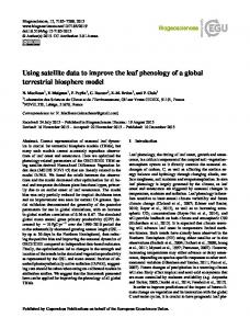
ative (Fig. 1a). If subfreezing cloud is detected, then the infrared cloud-top temperature is compared to the temperatures of the three geopotential surfaces. If the cloudtop temperature is greater than the model’s temperature at that level, then the level is assumed to be cloud and icing free (Fig. 1b). Thus, a first-guess indication of icing is changed to negative at that model level. Model levels below the cloud top retain a positive icing indication if so indicated by the first-guess field. If the cloud temperature is less than the model’s temperatures at all levels, then positive icing predictions are retained everywhere (Fig. 1c). The screening process is conservative in that it does not introduce new regions of potential icing; it only reduces the horizontal and vertical extent of the first-guess indication where the satellite analyses indicate subfreezing clouds are absent. Figure 2 presents an illustration of the two icing products. The first, standard icing output by the algorithm, is shown for the 850- (Fig. 2a) and 700-mb (Fig. 2b) levels. The light gray shading denotes the region for which there is satellite data (recall these data are from polar-orbiting satellites and therefore appear as ‘‘swaths’’) and no icing indicated, while the darker shading denotes a positive icing indication. When combined with the satellite cloud/no-cloud analysis, the resultant fields appear similar except some portions of the predicted icing have now been deleted. These ‘‘deleted’’
FIG. 1. Under the assumption that the model first guess indicates icing at 850, 700, and 500 mb for all three hypothetical regimes, satellite screening results in the following. (a) Satellite detects no clouds; therefore, the icing threat is removed at all three levels. (b) Satellite infrared temperature indicates cloud top below 700 mb; therefore, the threat is removed at 700 and 500 mb and kept at 850 mb. (c) Satellite infrared temperature indicates cloud top above 500 mb; therefore, the threat is kept at all three levels.
188
WEATHER AND FORECASTING
VOLUME 12
FIG. 2. Icing product depiction at 1300 UTC 24 January 1994 at 850 mb (a),(c) and 700 mb (b),(d) pressure levels. The first-guess, standard RAP icing algorithm is shown in (a) and (b), whereas the satellite screened product is shown in (c) and (d). Light gray shading denotes the region for which there is satellite data but no icing potential, while the darker gray shade denotes a positive icing indication.
regions are attributable to the lack of clouds with subfreezing tops in the satellite analysis. Referring to Fig. 2, notice that at 700 mb the standard product depicts icing over the entire state of Idaho (Fig. 2b), whereas the screened product (Fig. 2d) shows that most of Idaho has no icing potential (i.e., it is cloud free). The verification procedure applied to the two icing products follows that of B. Brown et al. (1997, manuscript submitted to Wea. Forecasting). Pilot reports (PIREPs) of icing are checked against the icing indicated by the algorithm–model couplet. If icing is predicted at any of the four grid points surrounding the PIREP location, then the PIREP is assigned a ‘‘hit.’’ If none of the surrounding points contain predicted icing, the PIREP is assigned a ‘‘miss.’’ Continuing this PIREP matching, a table of observed and forecast icing along with hits and misses is constructed. From this table, a TABLE 1. Satellite screening: overall results. All hours combined for 25 Jan–2 Feb 1994 (51 cases).
PODAll PODMOG PODNo Average area (106 km2) Average volume (106 km3) Average area efficiency
RAP
Screened RAP
% change
0.66 0.70 0.45 1.95 5.07 0.36
0.56 0.62 0.57 1.17 2.91 0.53
215 211 126 240 242 —
probability of detection (POD) can be estimated. However, because of the nature of the PIREP database (e.g., nonsystematic observations), the false alarm ratio cannot be computed (B. Brown et al. 1997, manuscript submitted to Wea. Forecasting). Instead, the area coverage of icing potential is used as a surrogate measure of overforecasting. To a large extent, the results of this study will rely on these two statistical measures. 3. Results A total of 51 cases were analyzed over a 10-day period from 24 January to 2 February 1994 (corresponding to individual swaths of the NOAA polar-orbiting satellites) and the overall results are shown in Table 1. The results from the standard algorithm (no cloud screening) are given in the column labeled ‘‘RAP.’’ Approximately 66% of all PIREPs were detected in this manner while impacting, on average, approximately 1.95 3 106 km2 in terms of area coverage. Taking a subset of the PIREPs and retaining only those PIREPs with moderate-orgreater severity (labeled PODMOG), 70% were detected. These quantities were also computed for the satellitescreened icing product (labeled ‘‘Screened RAP’’ in Table 1). The modified icing product detected 56% of all PIREPs (62% of moderate or greater severity) for all 51 cases combined, while impacting an average area of only 1.17 3 106 km2. That translates to a 40% smaller
MARCH 1997
NOTES AND CORRESPONDENCE
FIG. 3. Scatterplot of the 51 cases analyzed with percent probability of detection (POD) difference vs percent area coverage difference. All points lying to the right of a line that rises upward from the bottom-left corner to the upper-right corner represent cases with a greater decrease in area coverage than the corresponding decrease in POD (i.e., the satellite screen technique improved the first-guess field).
average area coverage while only decreasing the PODAll by 15% (11% for PODMOG). Furthermore, by dividing the POD by the average area coverage, an area efficiency measure can be calculated. This measure can be interpreted as the POD per unit area. Using this measure, the standard RAP product results in an overall area efficiency of 0.36 while the screened product scores 0.53. Another important result shown in Table 1 is a probability of detection of ‘‘no’’ PIREPs—labeled PODNo. The screened product scores higher, a 26% increase over
189
the nonscreened product. Again, comparing this percentage change against that of the PODAll (decrease of 15%), a larger impact on the PODNo is evident compared to the POD of positive icing reports. Using the satellitescreened product, the accuracy of the predicted ‘‘no icing’’ has increased more than the corresponding loss in accuracy of the predicted positive icing. To further illustrate the advantages of the screened product, the percentage change in POD from the nonscreened to the screened prediction can be plotted versus the percentage change in area as in Fig. 3. Here, the 51 cases are plotted and the clustering of points in the lower half of the figure indicates that a majority of the cases have a relatively large difference in area coverage yet a smaller difference in PODMOG from the standard to the screened icing product. Notice that there are 16 cases in which the area changed by a large amount yet the PODMOG did not change at all (dots along the lower horizontal axis). Generally, any point to the lower right of a diagonal line rising from left to right indicates a greater percentage change in area than in PODMOG, thereby accomplishing the main objective. As an illustration of one of the cases presented in Fig. 3, a case study from 2100 UTC 2 February 1994 is presented. Figure 4 shows the icing potential from both the standard (Figs. 4a and 4b) and screened (Figs. 4c and 4d) RAP algorithms. Notice the difference in area coverage particularly over the midwest United States. Statistically, there is a 52% decrease in area between the two products, yet the PODMOG remains the same (corresponding to the point along the x axis on Fig. 3 at a value of 52%).
FIG. 4. Same as in Fig. 2 except for 2100 UTC 2 February 1994.
190
WEATHER AND FORECASTING
4. Conclusions/recommendations Based on the results presented here, it appears that the satellite screening technique does aid in the reduction of spatial coverage of icing potential, based on the automated T–RH algorithm used here. In doing so, it appears that the reduction in POD is much smaller than the corresponding reduction of area. Theoretically, POD should not be reduced at all; however, misdiagnosis of cloud-free regions, errors in locations of pilot reports, and the long time window necessary to collect sufficient icing PIREPs (3 h on both sides of the satellite overpass) for statistical verification account for these changes. Some areas are erroneously diagnosed as cloud free by the satellite cloud screens owing to the difficulty in detecting cloud over a snow-covered background. Modification of the cloud screens to detect clouds in these regions would unfortunately increase the risk that nonexistent clouds would be misanalyzed in other regions. Additionally, the long time window for PIREP collection degrades the POD since the clouds are moving while the satellite captures the clouds at one instant. Therefore, PIREPs collected 2 h after the satellite image could actually be in cloudy regions, while the satellite analysis would indicate that they are not. Finally, the PIREPs are not a truly satisfactory validation dataset; however, they are the only one available. Even a perfect nowcast of icing potential would receive a less than perfect score from PIREP validation. We have no intention that pilots view such a product prior to takeoff and use it as their sole guidance of locations of anticipated icing hazards. However, currently, a diagnostic icing product such as this could be placed in front of dispatchers or flight control personnel. Then, a textual translation could be relayed directly to the pilots of affected aircraft either in flight or on the ground. Just as current surface conditions are relayed to pilots via recorded messages, a description of affected areas could be relayed as well. In the future, there will be means for transmitting graphics directly to the cockpit. Therefore, with the current configuration of geostationary satellites, graphical products could be created every 15 min and relayed to the cockpit for a real-time nowcast of potential icing hazards. Because this study used a relatively small sample (51 cases collected over 10 days), it is recommended that this work continue with a longer duration study (including 2 months worth of data). Furthermore, the new GOES (Geostationary Operational Environment Satellites) series satellites provide an opportunity to perform this work over the entire United States (instead of the small swath provided by the polar-orbiting satellites) and 24 h day21 (Menzel and Purdom 1994; Ellrod 1995). This will allow a shorter time window for PIREP collection plus a plethora of additional cases since the GOES satellites provide images every half hour. Since a half hour is usually not long enough to collect sufficient PIREPs, perhaps interpolating (smearing in time)
VOLUME 12
the satellite analysis over the same duration of the PIREP collection will provide more accurate results. At the very least, this should eliminate the time window as a possible source of error. Acknowledgments. This research is sponsored by the National Science Foundation through an Interagency agreement in response to requirements and funding by the FAA’s AWDP. The support of the research cosponsor, Space and Naval Warfare Systems Command, under Program Element 0603207N, is gratefully acknowledged. The views expressed are those of the authors and do not necessarily represent the official policy or position of the U.S. government. REFERENCES Allen, R. C., P. A. Durkee, and C. H. Wash, 1990: Snow/cloud discrimination with multispectral measurements. J. Appl. Meteor., 29, 994–1004. d’Entremont, R. P., 1986: Low- and midlevel cloud analysis using nighttime multispectral imagery. J. Climate Appl. Meteor., 25, 1853–1869. Ellrod, G. P., 1995: Advances in the detection and analysis of fog at night using GOES multispectral infrared imagery. Wea. Forecasting, 10, 606–619. , 1996: The use of GOES-8 multispectral imagery for the detection of aircraft icing. Preprints, Eighth Conf. on Satellite Meteorology and Oceanography, Atlanta, GA, Amer. Meteor. Soc., 168–171. Eyre, J. R., J. L. Brownscombe, and R. J. Allam, 1984: Detection of fog at night using Advanced Very High Resolution Radiometer (AVHRR) imagery. Meteor. Mag., 113, 265–271. Goerss, J., and P. Phoebus, 1992: The navy’s operational atmospheric analysis. Wea. Forecasting, 7, 3–24. Hammil, T. M., R. P. d’Entremont, and J. T. Bunting, 1992: A description of the air force Real-Time Nephanalysis Model. Wea. Forecasting, 7, 288–306. Kleespies, T. J., 1995: The retrieval of marine stratiform cloud properties from multiple observations in the 3.9-mm window under conditions of varying solar illumination. J. Appl. Meteor., 34, 1512–1524. Kopp, T. J., T. J. Neu, and J. Lanicci, 1994: A description of the Air Force Global Weather Central’s surface temperature model. Preprints, 10th Conf. on Numerical Weather Prediction, Portland, OR, Amer. Meteor. Soc., 435–437. Lee, T. F., and J. R. Clark, 1995: Aircraft icing products from satellite infrared data and model output. Preprints, Sixth Conf. on Aviation Weather Systems, Dallas, TX, Amer. Meteor. Soc., 234–236. Menzel, W. P., and J. F. W. Purdom, 1994: Introducing GOES-I: The first of a new generation of Geostationary Operational Environment Satellites. Bull. Amer. Meteor. Soc., 75, 757–781. Olesen, F., and H. Grassl, 1985: Cloud detection and classification over oceans at night with NOAA-7. Int. J. Remote Sens., 6, 1435–1444. Rosmond, T. E., 1992: The design and testing of the Navy Operational Global Atmospheric Prediction System. Wea. Forecasting, 7, 262–272. Saunders, R. W., and K. T. Kriebel, 1988: An improved method for detecting clear-sky and cloudy radiances from AVHRR data. Int. J. Remote Sens., 9, 123–150. Schickel, K. P., H. E. Hoffman, and K. T. Kriebel, 1994: Identification of icing water clouds by NOAA AVHRR satellite data. Atmos. Res., 34, 177–183. Yamanouchi, T., S. Suzuki, and S. Kawaguchi, 1987: Detection of clouds in Antarctica from infrared multispectral data of AVHRR. J. Meteor. Soc. Japan, 65, 949–961.