University of Michigan ... Ann Arbor, MI 48109. San Jose, CA 95120. Abstract. In this paper, we explore the execution of pipelined .... that simulates the action of each individual tuple to go ..... a list of greedy functions of all relations is derived.
Using Segmented Right-Deep Trees for the Execution of Pipelined Hash Joins Ming-Syan Chen, Mingling Lo�, Philip S. Yu and Honesty C. Youngy IBM T. J. Watson Research Ctr. EECS Department� IBM Almaden Research Ctry P.O.Box 704 University of Michigan 650 Harry Road Yorktown, NY 10598 Ann Arbor, MI 48109 San Jose, CA 95120
Abstract In this paper, we explore the execution of pipelined hash joins in a multiprocessor-based database system. To improve the query execution, an innovative approach on query execution tree selection is proposed to exploit segmented right-deep trees, which are bushy trees of right-deep subtrees. We rst derive an analytical model for the execution of a pipeline segment, and then, in light of the model, develop heuristic schemes to determine the query execution plan based on a segmented right-deep tree so that the query can be ef ciently executed. As shown by our simulation, the proposed approach, without incurring additional overhead on plan execution, possesses more exibility in query plan generation, and leads to query plans of signi cantly better performance than those achievable by the previous schemes using right-deep trees.
1 Introduction In relational database systems, joins are the most expensive operations to execute, especially with the increases in database size and query complexity [13] [15] [26]. Several applications involving decision support and complex objects usually have to specify their desired results in terms of multi-join queries, and some complex queries for such applications may take hours or even days to complete, thus degrading the system performance. As a result, parallelism has been recognized as the solution for the e�cient execution of multi-join queries for future database management [2] [6] [7] [13] [22]. Intra-operator parallelism, which occurs when several processors work in parallel on a single two-way join operation, was the focus of most prior studies on exploiting parallelism for database operations [1]
[5] [10] [14] [16] [18] [20]. In addition, inter-operator parallelism allows that several joins within a query be executed in parallel. Despite its importance, interoperator parallelism did not attract as much attention as intra-operator parallelism. This can be in part explained by the reasons that in the past the power/size of a multiprocessor system was limited, and the query structure used to be too simple to require further parallelizing in the inter-operator level. Notice, however, that those two limiting factors have been phased out by the rapid increase in the capacity of multiprocessors and the trend for queries to become more complicated nowadays, thus justifying the necessity of exploiting inter-operator parallelism [4] [9] [11] [17] [21]. Similarly to the study on intra-operator parallelism, to explore inter-operator parallelism, one has to consider the join methods employed. Among various join methods, the hash join has been elaborated upon by much research e�ort and reported to have superior performance to others [5] [14] [24]. Moreover, for exploiting inter-operator parallelism, hash joins provide the feasibility of pipelining. Using hash joins, multiple joins can be pipelined so that the early resulting tuples from a join, before the whole join is completed, can be sent to the next join for processing. A detailed description of pipelined hash joins and their advantages can be found in Section 2. Though pipelining has been shown to be very e�ective in reducing the query execution time, as will be described later, prior approaches on the implementation of pipelined hash joins are usually con ned to a linear order of relations involved, thus not fully exploiting the exibility on query plan generation. Consequently, in response to the increasing demand for a better performance of database operations, to study and improve the execution of pipelined hash joins for multi-join queries in a multiprocessor system is taken as the objective of this paper.
final resulting relations outer relations inner relations
R R 5 5 R 4 R3 R1 R2 (a) left-deep tree
R 4
R1 R2
R3 R2
R3
R 5 R 4
R1
(b) right-deep tree
(c) bushy tree
Figure 1: Illustration of di�erent query trees. The execution of a query can be denoted by three forms of query execution trees: left-deep trees, rightdeep trees, and bushy trees. In a query tree, a leaf node represents an input relation and an internal node represents the resulting relation from joining the two relations with its two child nodes, and the query tree is executed in a manner of bottom up. In the context of hash joins the left and right child nodes of an internal node denote, respectively, the inner and outer relations of a join [19], where, as explained in Section 2, the inner relation is the relation used to build the hash table and the outer relation is the one whose tuples are applied to probe the hash table. Examples of the three forms of query trees are shown in Figure 1, where the inner and outer relations are indicated for illustration. It can be seen that both right-deep and bushy trees allow the implementation of pipelining. Schneider and DeWitt are among the rst to study the e�ect of pipelining [19] [21], where the focus was on the use of right-deep trees due mainly to the simplicity of right-deep trees and the uncertainty for the improvement achievable by using bushy trees. Clearly, for a given query, the number of right-deep trees to be considered is signi cantly less than that of bushy trees, and simple heuristics can be applied with little overhead to generate a right-deep query plan. For example, a right-deep tree can be obtained by rst constructing a left-deep tree by some greedy methods and then taking a mirror image of the resulting left-deep tree [19]. However, right-deep trees might su�er from the drawback of less exibility on structure, which in turn implies a limitation on performance. Moreover, since the amount of memory is usually not enough to accommodate hash tables of all inner relations, special provisions, such as static right-deep scheduling and dynamic bottom-up scheduling [21], are needed to deal with this problem. In both scheduling methods, a
right-deep tree is decomposed into disjoint segments in such a way that for each segment the hash tables of its inner relations can be tted into memory.1 For these methods, however, the execution of the whole query is implemented in one pipeline and thus restricted to the structure of a right-deep tree. An example right-deep tree which is decomposed into three segments is shown in Figure 2a, where one hash join is called a pipeline stage and several stages form a pipeline segment. The pipeline segments are executed one by one in a manner of bottom up with all resources in the system devoting to one segment at a time. Those joins whose resulting relations need to be written back to disks are marked black in Figure 2a for illustration. The bushy tree, on the other hand, o�ers more exibility on query plan generation at the cost of searching a larger space. It has been shown that for sort-merge joins, the execution of bushy trees can outperform that of linear trees, especially when the number of relations in a query is large [4]. However, as far as the hash join is concerned, the scheduling for an execution plan of a bushy tree structure is much more complicated than that of a right-deep tree structure. Particularly, it is very di�cult, if not impossible, to achieve the synchronization required for the execution of bushy trees such that the e�ect of pipelining can be fully utilized. This is the very reason that most prior studies on pipelined hash joins focused on the use of right-deep trees. As an e�ort to improve the execution of pipelined hash joins, one would naturally like to develop e�cient schemes to generate e�ective query plans that fully exploit the advantage of pipelining while avoiding the above mentioned de ciencies of the bushy and right-deep trees. Consequently, we propose in this paper the approach based on segmented right-deep trees for the execution of pipelined hash joins. A segmented right-deep tree is a bushy tree which is composed of a set of right-deep subtrees. An example of a segmented right-deep tree of 3 pipeline segments can be found in Figure 2b. A segmented right-deep tree is similar to a conventional right-deep tree in that all processing nodes execute one pipeline segment at a time, hence not incurring additional overhead on plan execution, but di�ers from the latter in that the resulting relation of a pipeline segment in the former can be either an inner relation or the outer relation of any of the subsequent segments, thus possessing the 1 While the static right-deep scheduling decomposes the right-deep tree into segments o�-line and loads hash tables of a segment into memory in parallel, the dynamic bottom-up scheduling loads one hash table into memory at a time and determines the break points of segments dynamically according to the memory constraint.
J8
J8 J7
J7 J5
J6
J6 J4
J5 J4
J3
join is also investigated by simulation. Preliminaries are given in Section 2. The execution model for a pipeline segment is derived in Section 3.1, and heuristics for relation selection are developed in Section 3.2. Performance of these heuristic schemes is evaluated by simulation in Section 4, followed by the conclusion in Section 5.
J3 J2
J2
J1
pipeline stage
J1
pipeline segment (a)
(b)
Figure 2: (a) a conventional right-deep tree, and (b) a segmented right-deep tree.
exibility of a bushy tree. Note that unlike the generation of right-deep trees that can resort to the similar heuristics for generating left-deep trees, to schedule a pipelined hash joins based on segmented rightdeep trees, we have to develop new heuristic schemes. Speci cally, we shall rst estimate the number of segments to be employed in a query plan, and then determine the relations that participate in each pipeline segment. Clearly, this problem is much more complicated than the one to select a pair of joining relations at a time in building a linear tree, since both a subset of relations and their join order have to be determined. To deal with this, we shall derive an analytical model for the execution of a segmented right-deep tree, and then, in light of the model, develop e�cient heuristics for relation selection for each pipeline segment. It will be seen that under the execution of a segmented right-deep tree not only is the synchronization problem completely resolved, but also processor fragmentation [4] is avoided. As evaluated by our simulation that simulates the action of each individual tuple to go through the pipeline, the proposed approach on segmented right-deep trees, without incurring additional overhead on plan execution, possesses more exibility in query plan generation, and is favorably compared with not only the right-deep trees generated by greedy methods but also the optimal right-deep tree that has the shortest execution time among all right-deep trees. This fact strongly suggests that to e�ciently execute pipelined hash joins for years to come, instead of improving the heuristics on generating right-deep trees, one has to exploit the methods utilizing the bushy trees, such as the one proposed in this paper. The e�ect of processor allocation for the execution of each
2 Preliminaries We assume that a query is of the form of conjunctions of equi-join predicates. A join query graph can be denoted by a graph G = (V, E), where V is the set of nodes and E is the set of edges. Each node in a join query graph represents a relation. Two nodes are connected by an edge if there exists a join predicate on some attribute of the two corresponding relations. We use jRij to denote the cardinality of a relation Ri and jAj to denote the cardinality of the domain of an attribute A. As in most prior work on the execution of database operations, we assume that the execution time incurred is the primary cost measure for the processing of database operations. Also, we focus on the execution of complex queries [23], i.e., queries involving many relations. Notice that such complex queries can become frequent in real applications due to the use of views [26]. The architecture assumed is a multiprocessor system with distributed memories and shared disks. Each processing node, or processor, in the system has its own memory and address space, and communication between nodes is done by message passing. The amount of memory available to execute a join is assumed to be in proportion to the number of processors involved. In addition, we assume for simplicity that the values of attributes are uniformly distributed over all tuples in a relation and that the values of one attribute are independent of those in another. Thus, when the heuristics derived in Section 3.2 are applied, the cardinalities of resulting relations of joins can be estimated according to the formula used in prior work [3] that is given in the Appendix for reference2 . In the presence of data skew [25], we only have to modify the corresponding formula accordingly [8]. For ease of exposing the concept of segmented right-deep trees, we assume the aggregate memory in the system can accommodate a few entire relations for pipelining. Note that in the case that the aggregate memory is not 2 This formula is employed to be consistent with the generation of each output tuple of a join under our simulation in Section 4. Note that this o�ers a more sophisticatedmodel than the one based on the foreign key assumption.
notation jRij S Rh Ii q m N k ni i
meaning cardinality of a relation Ri outer relation of the segment inner relation of stage i intermediate relation from stage i number of relations in a query number of segments in an SRD total number of nodes in the system number of stages of a segment number of nodes allocated to stage i
Table 1: Notation for the execution of a pipeline segment. large enough to load some entire relations, one can still utilize the structure of segmented right-deep trees for more exibility on plan generation, and employ the techniques, such as right-deep hybrid scheduling [19], to resolve the memory constraint and implement one pipeline segment at a time to exploit pipelining. The execution of a hash join consists of two phases: the table-building phase and the tuple-probing phase. In the table-building phase, the hash table of the inner relation is built according to the hash function of the join attribute, and in the tuple-probing phase each tuple of the outer relation is applied by the hash function and used to probe the hash table of the inner relation for matches. In the context of hash joins, the left and right child nodes of an internal node in a query execution tree denote, respectively, the inner and outer relations of a join. It can be seen that in a left-deep tree, the result of a join is used to build the hash table for the next join, and several hash joins thus need to be executed sequentially. In contrast, in a right deep tree all the hash tables are built from the original input relations, and the resulting relation of a join is input into the next join as an outer relation. The tuples of the outer relation can thus go through the whole right-deep tree in a manner of pipelining. The bushy tree, on the other hand, is not restricted to a linear form, meaning that the resulting relation of a join in the bushy tree does not have to be immediately used in the next join. The resulting relation of a join can in fact be used as either an inner or an outer relation for subsequent joins. Recall that a segmented right-deep tree is a bushy tree of right-deep subtrees. Each right-deep subtree is a pipeline segment comprising of a number of pipeline stages (joins). Also, q is the number of relations in a query, m is the number of segments in a segmented
right-deep tree, and N is the total number of processing nodes in the multiprocessor system. The analytical model to be derived is for one pipeline segment where k is used to denote the number of stages in the segment, and ni is the number of nodes allocated to stage i. In what follows, S represents the outer relation of the segment. Rh and Ii denote, respectively, the inner relation and the intermediate resulting relation at stage i, where the value of jIi j can be obtained by the formula in the Appendix. These symbols are summarized in Table 1. The table-building phase and the tuple-probing phase of the execution of a pipeline segment are described below. Table-building phase In this phase, the hash tables of all stages are built. If more than one node is allocated to a stage, the hash table for that stage is hashed into many partitions using a partition function in such a way that one processing node deals with one partition of the hash table. The tuples in each partition are then hashed and built into a hash subtable. This phase is composed of the following two steps. 1. All the nodes read inner relations Rh , for i = 1; : : :; k, from disks. When a node reads one block of relation Rh from a disk, that node uses the partition function of stage i to hash the tuples in the block into a number of partitions. The partitioned tuples are then sent to their destination nodes in stage i. 2. Each node in stage i, for i = 1; : : :; k, receives the tuples of its corresponding partition, hashes those tuples with the hash function of the stage (join) and inserts these tuples into the hash subtable. i
i
i
Tuple-probing phase After the table-building phase, the pipeline segment starts tuple probing as described below. 1. The blocks of the outer relation S are read from disks, partitioned with the partition function of stage 1 and routed to the corresponding nodes in stage 1. The tuples are sent to their destination nodes whenever there are enough tuples to form a communication packet. 2. For each node in stage i, where i = 1; : : :; k ? 1, whenever a packet of input tuples is received, those tuples are probed, one by one, against the subtable using the hash function of stage i. If there are matches, the intermediate resulting tuples are generated. These intermediate tuples are then partitioned with the partition function of the next stage, i.e. stage i + 1. When the number of
n3 =4 n 2=2 R
3 R
n 1 =3 1 R 2
S
k=3
h 1 =2
N=9
h 2 =1 h 3 =3
R2
processing nodes packets
R3
R1 disks
S
stage 2 stage 1 stage 3
Figure 3: Execution of one pipeline segment. tuples in the output queue to a certain node in the next stage is enough to form a packet, that packet is sent to its destination node. 3. The nodes in stage k receive their input tuples, probe them against the subtables and generate the resulting tuples when there are matches. Note that the resulting relation of this stage is the resulting relation of the whole segment. The resulting tuples are written back to disks block by block. Pipelining has the following two advantages. First, the disk I/O cost is signi cantly reduced since the intermediate relations between stages in a segment need not be written back to disks. Second, the rst tuples of the resulting relation of a pipeline segment can be produced earlier, not only reducing the perceived response time by an end user, but also enabling an application program to start processing the result earlier. The execution of the rst pipeline segment of the segmented right-deep tree in Figure 2b is shown in Figure 3.
3 Pipelined Hash Joins for SRD Trees 3.1 Model of a Pipeline Segment We now analyze the cost and elapsed time in both the table-building phase and the tuple-probing phase for a pipeline segment. Various timing parameters referenced in this analysis are given in Table 2. Recall that the table-building phase consists of two steps. In the rst step, all nodes read from the disks the inner
para. tread tpart tsend trec thash tinsert tcomp tbuild twrite C1 C2 C3 C4 C5
meaning cost of reading one tuple from disk. cost of applying partition functions. cost of sending a tuple to the network. cost of receiving one tuple from network. cost of applying hash functions. cost of tuple insertion to a hash subtable. cost of tuple comparison. cost of building a resulting tuple. cost of writing one tuple to disk. tread + tpart + tsend trec + thash + tinsert trec + thash + tcomp tbuild + tpart + tsend tbuild + twrite Table 2: A list of timing parameters.
relations, partition and send them to the destination nodes according to the partitioning functions of the corresponding join P attributes. The total amount of work in this step is ki=1 jRh j � (tread + tpart + tsend), and the amount of work by the nj nodes of stage j is P k thus i=1 jRh j� (tread +tpart +tsend ) � nN . In the second step, the nodes in each stage receive the tuples of the corresponding inner relation, hash them, and build hash subtables for these P tuples. The total amount of work in this step is ki=1 jRh j� (trec +thash +tinsert). Since the nodes of stage j are only associated with the work related to Rh , the amount of work by the nodes of stages j can be expressed as jRh j � (trec + thash + tinsert). Denote the total work by all the nodes in the table building phase as WB. Then, i
j
i
i
j
j
WB = (C1 + C2)
k X i=1
jRh j; i
where C1 and C2 are system dependent parameters given in Table 2. The amount of work performed by the nodes of stage j in the table-building phase is WBj = C1
k X i=1
jRh j � nNj + C2 � jRh j: j
i
Denote the table-building time at stage j as TBj . Then,
Pk jR j C jR j C 1 i=1 h + 2 h : TBj = N nj i
j
The elapsed time in the table-building phase TB can then be approximated by the maximum of all TBj . Thus, we have, TB = max8j TBj : Next, the total amount of work in the tuple-probing phase, WP, can be derived similarly from the description in Section 2. We get, WP = (C1 + C3)jS j + (C3 + C4 )
kX ?1 i=1
jIij + C5 jIk j;
where C3; C4 and C5 are system dependent parameters given in Table 2. The amount of work by the nodes of stage j in the tuple-probing phase can be expressed as: WPj =
(
C1 jS j�nj C1 jN S j�nj N
+ C3jIj ?1j + C4jIj j if j 6= k; + C3jIj ?1j + C5jIj j if j = k:
Note that the processing time of the tuple-probing phase for each stage in the pipeline includes three parts. The rst part is the time to set up the pipeline, the second part is the steady state processing time, and the third part is the pipeline depletion time. For large relations, it can be seen that all stages spend most of their time in steady state processing. Also, note that in the steady state, in addition to processing inputs and producing outputs, a node could be idling due to the following scenarios. First, since only a nite amount of communication bu�er space is available in each node, if, at any instant, the input bu�er of a certain node is full, any processing in the preceding stage to produce further input to that node needs to stall to avoid loss of information. On the other hand, when the input bu�er of a node is empty, that node, since it has completed the processing for all prior tuples, will be starved and waiting for inputs from nodes in the preceding stage to proceed. It can be seen that these scenarios, resulting from the burst e�ects of hash joins, are very dependent on the characteristic of each individual query, and believed to be very di�cult, if not impossible, to have a general model to capture. Therefore, we shall only model the non-idling steady state processing time below. The burst e�ects of hash joins will be captured via simulation in Section 4. Denote the non-idling steady state processing time of a stage i as TPi . Then, we have, TPi =
(
C1 jS j + C3 jIi?1 j+C4 jIij N n C1 jS j + C3 jIi?1 ji+C5 jIij N ni
if i 6= k; if i = k:
Denote the processing time of the tuple-probing phase as TP. Since the pipeline set-up and depletion times
are negligible as compared to the steady state processing time, the processing time of the tuple-probing phase TP can be approximated as: TP = max8i TPi: Consequently, the total processing time for a pipeline segment TS can be expressed by the sum of the processing times in the table-building and the tupleprobing phases: TS = TB + TP = max TBi + max TPi: (1) 8i 8i
The total processing time for a query TQ is the sum of the processing times of all its segments. Thus, m X TQ = TSj ; j =1
where m is the number of pipeline segments, and TSj is the processing time of the jth segment.
3.2 Plan Generation for SRD Trees As pointed out earlier, unlike the generation of right-deep trees which can use the similar heuristics for generating left-deep trees, new heuristics need to be developed to build e�ective segmented right-deep trees. Speci cally, we shall rst estimate the number of pipeline segments, and then select the inner and outer relations for each pipeline segment so as to minimize the query execution time. The size of all relations and that of the total memory need to be considered in estimating the number of segments required. It is shown by our experiments that too many segments can result in worse performance. This can be explained by the reason that for each pipeline segment, there are overheads of setting up hash tables, lling and depleting the pipeline segment, and writing the resulting relation of the segment back to disks. These overheads usually outweigh the possible advantages we can gain from the exibility of having more segments. Thus, the estimated number of segments, m, is chosen to be close to the number ofPsegments enough to hold all the relations, i.e., m = d N=1�MjR j e, where M is the memory size of each processing node. After the number of segments is estimated, we set an upper bound, k, for the projected number of relations in each segment by k = d mq e. Note that m and k are projected numbers to be used in our heuristic schemes below, and might be di�erent from those in the nal plans generated. Such a projection avoids making the memory in the early stages always fully loaded, and usually leads to a better performance due to a better load balancing. q i
i
Selecting relations for a pipeline segment amounts to selecting a subset of relations, and is more complicated than selecting a pair of relations in building a right-deep tree. To cope with this, we propose greedy approaches to handle the problem of relation selection for each segment. The relations are selected one by one until either all the k relations in the segment are determined or the total size of inner relations becomes greater than that of the total memory available. In the segmented right-deep tree generated, the intermediate relation resulting from each segment can appear as either an inner or the outer relation of any of the subsequent segments, whereas in a conventional rightdeep tree the resulting relation from a segment can only be used as the outer relation in the next segment. Based on the model derived in Section 3.1, we propose the following two heuristics, namely, the minimal work (MW) and the balanced consideration (BC), to determine the segmented right-deep tree.
3.2.1 Heuristic on minimal work
The objective of MW is to select relations in the segment so that the total amount of work involved in its stages is minimized. Speci cally, given a set of relations and the number k, we determine a sequence of up to k inner relations and one outer relation so as to minimize the total work W. Note that, W = WB + WP
k X
jRhi j + (C1 + C3)jS j i=1 kX ?1 +(C3 + C4) jIij + C5jIk j; i=1
= (C1 + C2 )
is a linear combination of jS j, jRh j, and jIi j, for i = 1; : : :; k. Therefore, we can decompose W into groups of terms related to relations S, Rh1 ; Rh2 ; : : :, and Rh . When determining an inner or the outer relation, we select a relation that minimizes the sum of the terms related to itself and the intermediate relation resulted by this selection. For example, when selecting the relation for the second stage, Rh2 , we choose a relation to minimize the terms in W that are related to Rh2 and I2 , since I2 is determined by the selection of Rh2 . Relations are selected in the order of Rh1 ! S ! Rh2 ! Rh3 ! � � � ! Rh . The sum of those terms to be minimized when selecting a certain relation is called the greedy function of that relation. Under MW, a list of greedy functions of all relations is derived and given in Table 3. It can be seen that the greedy i
k
k
heur. relation Rh1 MW S Rh , i 6= 1; k Rh Rh1 BC S Rh , i 6= 1; k Rh i
k
i
k
greedy function jRh1 j (C1 + C3 )jS j + (C3 + C4)jI1 j (C1 + C2 )jRh j + (C3 + C4)jIi j (C1 + C2 )jRh j + C5jIk j jRh1 j jI1 j (C2 ? C3 )jRh j + (C3 + C4)jIi j (C2 ? C3 )jRh j + C5jIk j i
k
i
k
Table 3: The greedy function of each relation for heuristics MW and BC. functions are determined according to the selection order of relations. Note that the criteria for selecting di�erent relations are di�erent, which agrees with our intuition since these relations play di�erent roles in a pipeline segment and have di�erent in uences on performance. The complexity of heuristic MW can be shown to be O(q2 ), where q is the number of relations in the query. To illustrate heuristic MW, consider an example query of 7 relations whose pro le is given in Figure 4 and Table 4. We assume a multiprocessor system of eight nodes is employed, where each node has 64K byte memory and the size of each tuple is assumed to be 100 bytes3 . The query plans generated by a rightdeep tree approach and MW are shown in Figure 5a and Figure 5b, respectively. For this example query, the right-deep heuristic builds a six stage pipeline rst, and then divides this pipeline into three segments according to the memory constraint as shown in Figure 5a. Heuristic MW, on the other hand, is able to use the resulting relations of earlier segments as hash tables for later segments. For instance, in the query plan in Figure 5b, the resulting relation of the rst segment (of 397 tuples) is used as the inner relation of the rst stage of the next segment due to its relatively small size, whereas that in Figure 5a is used as the outer relation of the next segment. It can be veri ed that the total size of hash tables for the segmented right-deep tree in Figure 5b is smaller than that of the rightdeep tree in Figure 5a. Note that a smaller hash table size usually leads to a shorter query execution time for pipelined hash joins. Simulation, conducted in Section 4, shows that for the query in Figure 4, the processing 3 The reason to scale down the memory size is explained in Section 4. The assumption for the xed tuple size is for ease of exposition, and not essential for the improvement achieved by the proposed schemes.
R6 G R5
R1
R2 A
F
E
B
R4
R3
D C
R7
Figure 4: An example query with 7 relations Ri R1 R2 R3 R4 R5 R6 R7 card. 1137 802 1840 1633 884 1426 1251 (a). Cardinalities of relations. attr. A B C D E F G card. 1494 1943 1646 1651 1478 1028 1325 (b). Cardinalities of attributes. Table 4: The pro le of the example query in Figure 4. time under the right-deep tree in Figure 5a is 74.59 msec, and that under MW in Figure 5b is 48.46 msec. As indicated by the simulation in Section 4, performance of MW is reasonably good but not always stable. This is due to the fact that MW tends to select smaller relations rst for early segments. This may lead to two disadvantages. First, because those relations selected for later segments have larger sizes, it might happen that the total memory available is not enough to hold all inner relations, so that additional segments are required, leading to more segments than projected and a longer query execution time. Second, the rst few segments have smaller relations, which might result in under-utilization of memory. Such scenarios are more likely to occur when the sizes of relations vary drastically.
3.2.2 Heuristic on balanced consideration
To eliminate this instability of MW, we propose heuristic BC which avoids the tendency of selecting small relations for the rst few segments. In BC, a penalty P and a bene t B are de ned for each segment. The penalty is de ned as the work in the segment, i.e., WP +WB, and the bene t is de ned as the size reduction after the execution of this segment, i.e., (jS j + jRh1 j + jRh2 j + � � � + jRh j) ? jIk j. The relations k
R3
R6
R 5 R 1
R 7 R 5 R 2
(a)
R 4 R 6
R 3 R 4
R 3 R 4 R 6 R 7 R 5 R 1
R 2 (b)
R 1
R 2
R 7
(c)
Figure 5: The resulting query execution trees: (a) right-deep tree plan, (b) MW, and (c) BC. are selected in such a way that the objective function Y = P ? w � B is minimized, where w is a weighting factor. Since the relations that give larger reduction on relation size are not necessarily those smaller relations, balanced consideration on both bene t and penalty avoids the tendency of selecting all small relations for the rst few segments. Determining the weight w in the objective function Y represents another degree of freedom for tuning the heuristic. In the simulation in Section 4, w = C1 +C3 is used for its reasonably good performance, and the coe�cient for jS j in objective function Y is thus zero. The greedy functions for heuristic BC are derived and given in Table 3. Eliminating the terms involving jS j from the objective function means that \small relation size" itself will not be taken as the factor in selecting the outer relation S. Note that in a hash join, using the smaller of the two joining relations as the inner relation usually results in better performance. For the example query in Figure 4, the resulting query tree by BC is given in Figure 5c. The query trees generated by MW and BC for this query have the same shape, but di�erent join orders of relations. It is obtained by simulation that the processing time for this query under BC in Figure 5c is 47.06 msec. Performance of these heuristic schemes is assessed in Section 4. Clearly, it is possible to further improve the above query processing during actual implementation. For instance, during the rst step of the table-building phase, we can assign those nodes at stage i to read the blocks of relation Rh so as to reduce the number of tuples to be transferred over the network. In addition, the work in the rst step of the tuple-probing phase could be dynamically assigned to the nodes that have the lowest load at that instant. Optimization on i
these issues is rather system dependent, and thus not addressed in this paper.
4 Simulation
4.1 Description of Simulation Model
Extensive simulations were performed to evaluate the heuristic schemes for query plan generation. In the simulation program, which was coded in C, the action for each individual tuple to go through all stages in a pipeline was simulated. Input queries were generated as follows. The number of relations in a query was predetermined. The occurrence of an edge between two relations in the query graph was determined according to a given probability, denoted by prob. Without loss of generality, only queries with connected query graphs were deemed valid and used for our study. To determine the cardinalities of relations and attributes, we referenced a workload recently generated from the work at a Canadian insurance company. To make the simulation able to be feasibly conducted in a tupleby-tuple manner, we scaled the average number of tuples in a relation down from one million to two thousand. The cardinalities of attributes and the memory size of each processing node were also scaled down accordingly so that the ratio of the relation size to the memory size could still re ect the reality. Based on the above, the cardinalities of relations and attributes were randomly generated from a uniform distribution within some reasonable ranges. In the simulation program, for each query we generated query trees of two styles, i.e., static right-deep trees and segmented rightdeep trees. For the static right-deep tree, both the greedy right-deep tree that is constructed by a greedy method and the optimal right-deep tree were evaluated. The greedy method used is to rst construct a left-deep tree by the heuristic on minimal resulting relation [3] and then take the mirror image of the left-deep tree to form a right-deep tree. Both rightdeep trees were decomposed according to the static right-deep scheduling described in Section 1. Recall that the optimal right-deep tree is the right-deep tree that has the shortest processing time among all rightdeep trees, whose identi cation is of exponential time complexity. For the segmented right-deep tree, both heuristics MW and BC were employed. To allocate processors to the execution of both right-deep and segmented right-deep trees, we consider two alternatives. The rst approach is to allocate to each stage the number of nodes enough to hold the hash table, and then distribute the remaining nodes uniformly to
parameters �-seconds tread 50 tpart 4 tsend 4 trec 2 thash 4 tinsert 20 tcomp 2 tbuild 40 twrite 80 Table 5: CPU costs used in simulation. each stage. The second approach is to minimize the formula TS = TB + TP in Eq.(1) for each pipeline segment, which can be done by using a typical dynamic programming technique4 . It can be seen that fragmentation of processors is avoided since all nodes in the system are employed to implement one pipeline segment at a time. A query and an execution strategy are the inputs to the simulator. An execution strategy employed determines the number of segments, the inner and outer relations for each segment, and the number of nodes allocated to perform the hash join in each stage. In the table-building phase, the hash table for each stage was built in such a way that the corresponding inner relation was partitioned into subtables for those processing nodes in that stage. When the probing phase started, a random number generator was used to determine which subtable (processing node) the probing tuple should be routed to. A zero/one random number generator, which was coded based on the join selectivity, was then employed to determine the generation of resulting tuples, which were in turn, according to the next join attribute, sent to the subsequent stages for processing. To conduct the simulation, [14] and [19] were referenced to determine the values of the system parameters which are given in Table 5, and the network delay in sending a 2K byte packet, Dnet , is assumed to be 1 msec5. The behavior of pipelines can thus be predicted by the analytical model derived in Section 3.1. As pointed out in Section 3.1, due to 4 Tuning the number of processors allocated to each stage has an impact on overall performance, whose discussion is beyond the scope of this paper. Interested readers are referred to [12]. 5 Note that t read and twrite denote amortized CPU costs for processing one 100 byte tuple. Since asynchronous disk I/O is assumed, the I/O latency is not included in the model to facilitate our discussion. The packet size is chosen to be 2K byte to comply with the reduction of the memory size.
4.2 Simulation Results From our simulation, we rst observed the execution time for queries of four sizes, i.e., queries with 8, 12, 16 and 20 relations, in a multiprocessor system of eight nodes. For each query size, 100 query graphs were generated and each query was simulated twice. Simulation results for the average execution times of plans generated by the greedy right-deep tree (RD), the optimal right-deep tree (opt. RD), heuristics MW and BC are shown in Figure 6 where the system has 8 nodes and each node has 64K byte memory. It can be seen that MW and BC for segmented right-deep trees outperform both the greedy and the optimal rightdeep trees. The improvement of MW and BC over both right-deep tree becomes even more signi cant as the number of relations in a query increases. As shown in Figure 6, the execution time of BC ranges from 56% (when q=20) to 66% (when q=8) of that of RD. Note that some join plans might result in extraordinarily long execution time, thus a�ecting the fairness of using the average execution time as a measure for performance. To remedy this, we compared, for each query, the execution times resulted from the four schemes, and sorted them in an ascending order. Then, we assigned 0 to 3 points to each scheme in such a way that the number of points assigned to a scheme is the number of other schemes outperforming this scheme. Clearly, a scheme with fewer points performs better. Corresponding to Figure 6, the points assigned to each scheme are shown in Table 6. From Figure 6 and Table 6, it can be observed that MW performs rather close to BC while the latter is more stable in performance due to the balanced consideration on bene t and penalty, as described in Section 3.2.2. In the case that n=20, it is noted that opt. RD,
300
Execution time (msec)
the nature of pipelining, there can be, resulting from the burst e�ects of hash joins, various scenarios where processing nodes are starved for inputs or forced to stall because of the congestion in subsequent stages. These scenarios have an impact on the processing time and can only be observed by using the model which simulates the action of each tuple. This is the very reason that we, instead of relying upon the analytical model derived in Section 3.1, conducted the tuple-bytuple simulation to re ect the complicated nature of pipelined hash joins and obtain more realistic results. Nevertheless, the analytical model derived was found to be useful in deriving heuristics for query plan generation and also able to provide a reasonable prediction for the performance of a query plan.
250
RD
opt. RD
MW
BC
200 150 100 50 0
q=8
q=12
q=16
q=20
q: the number of relations in a query
Figure 6. Average execution time of plans generated by different schemes.
n=8 n=12 n=16 n=20
RD opt. RD 447 272 483 304 558 370 596 389
MW 248 218 144 117
BC 233 195 128 98
Table 6: The points assigned to each scheme. for the 200 instances examined, is only better than either MW or BC for about 10 instances. (Note that the points which opt. RD received would be 400, if it was always ranked in the third place.) The fact that MW and BC outperform the approach using optimal right-deep trees indicates that to e�ciently execute pipelined hash joins, instead of focusing on improving the heuristics on generating right-deep trees, one should utilize the bushy tree structure. In fact, for the sizes of queries investigated here, the simulation times (including plan generation and execution) for the schemes on RD, MW and BC were very close to each other whereas that of opt. RD was larger than others by orders of magnitude. It is noted that these results were obtained by assigning prob, i.e., the probability of the occurrence of each edge in a query graph, to be 0.26. The cases when prob=0.24 and prob=0.28 were also simulated. It was shown that the relative performance of these schemes was not sensitive to the value of prob. Performance charts for di�erent values of prob are thus not shown in the paper. As mentioned earlier, in light of the derivation in Section 3.1, the query execution time can be further improved by adjusting the number of processors allocated to each stage. This e�ect is shown in Figure 7, where a \*" is appended to the symbol of a scheme to mean the processor allocation was tuned to min-
for the execution of a query, and did not observe the necessity for executing more than one pipeline segment at a time. Clearly, when the number of processors is large, we might have to divide the multiprocessor system into several partitions, and use each partition to implement one pipeline segment to exploit multisegment parallelism for a better performance.
Execution time (msec)
300 250
RD
RD*
BC
BC*
200 150 100 50 0
q=8
q=12
q=16
q=20
q: the number of relations in a query
Figure 7. The effect of processor allocation.
stable
0.6
.590
Execution time ratio
.561
small variance
large variance
.563
.577 .546
.542
.518
0.5 .446
.442
.503
.440
.432
0.4
5 Conclusions We rst derived an analytical model for the execution of a pipeline segment, and then, developed heuristic schemes to build the segmented right-deep trees for e�cient query execution. As shown by our simulation, the proposed approach, without incurring additional overhead on plan execution, possesses more exibility in query plan generation, and leads to query plans of signi cantly better performance than those achievable by the previous schemes using right-deep trees.
0.3
Acknowledgement
0.2 0.1 0 q=8
q=12
q=16
q=20
q: the number of relations in a query
Figure 8. Improvement of BC* over RD (different variances on input relation sizes).
imize the TS in Eq.(1) according to a dynamic programming technique. It is indicated in Figure 7 that while processor allocation is important, the structure of query trees is still the major factor to minimize the query execution time. In addition, to realize the e�ect of variance on the input relation size, we compared performance of BC* and RD under di�erent variances on the cardinalities of relations, and showed the results in Figure 8, where the execution time of BC* was divided by that of RD for clarity. In Figure 8, the cardinalities of relations varied from 1800 to 2200 in the stable case, from 1400 to 2600 in the small variance case, and from 800 to 3200 in the large variance case. They represent 10%, 30% and 60% variations, respectively, from a mean of 2000. Di�erent query sizes with q=8, 12, 16 and 20 are considered. As can be seen in Figure 8, when the variance on relation cardinality increases, the improvement of BC* over RD becomes more prominent. For the input queries simulated here, we had one to ve relations in a segment and one to four segments
The authors would like to thank S. Lavenberg and J. Chen at IBM for their comments and assistance on improving the presentation of this paper.
References [1] C. K. Baru and O. Frieder. Database operations in a cube-connected multiprocessor system. IEEE Trans. on Computers, 38(6):920{927, June 1989. [2] H. Boral, W. Alexander, et al. Prototyping Bubba, a highly parallel database system. IEEE Trans. on Knowledge and Data Eng., 2(1):4{24, March 1990. [3] M.-S. Chen and P. S. Yu. Determining bene cial semijoins for a join sequence in distributed query processing. Proceedings of the 7th Intern'l Conf. on Data Engineering, pages 50{58, April 1991. To appear in IEEE Trans. on Parallel and Distributed Systems. [4] M.-S. Chen, P. S. Yu, and K.-L. Wu. Scheduling and processor allocation for parallel execution of multi-join queries. Proceedings of the 8th Intern'l Conf. on Data Engineering, pages 58{67, Feb. 1992. [5] D. J. DeWitt and R. Gerber. Multiprocessor hash-based join algorithms. Proceedings of the 11th Int'l Conf. on Very Large Data Bases, pages 151{162, Aug. 1985.
[6] D. J. DeWitt, S. Ghandeharizadeh, D. A. Schneider, A. Bricker, H.I. Hsiao, and R. Rasmussen. The Gamma database machine project. IEEE Trans. on Knowledge and Data Eng., 2(1):44{62, March 1990. [7] D. J. DeWitt and J. Gray. Parallel database systems: The future of high performance database systems. Comm. of ACM, 35(6):85{98, June 1992. [8] D. Gardy and C. Puech. On the e�ect of join operations on relation sizes. ACM Trans. on Database Syst., 14(4):574{603, Dec. 1989. [9] G. Graefe. Rule-based query optimization in extensible database systems. Technical Report Tech. Rep. 724, Computer Science Department, Univ. Wisconsin-Madison, Nov. 1987. [10] W. Hong and M. Stonebraker. Optimization of parallel query execution plans in XPRS. Proceedings of the 1st Conf. on Parallel and Distributed Information Systems, pages 218{225, Dec. 1991. [11] Y. E. Ioannidis and Y. C. Kang. Left-deep vs. bushy trees: An analysis of strategy spaces and its implication for query optimization. Proceedings of ACM SIGMOD, pages 168{177, May 1991. [12] M.-L. Lo, M.-S. Chen, C. V. Ravishankar, and P. S. Yu. Optimal processor allocation for the execution of pipelined hash joins. IBM Research Report, June 1992. [13] R. A. Lorie, J.-J. Daudenarde, J. W. Stamos, and H. C. Young. Exploiting database parallelism in a message-passing multiprocessor. IBM Journal of Research and Development, 1992. To appear. Also available as IBM RJ 8202, June, 1991. [14] H. Lu, K. L. Tan, and M.-C. Shan. Hashbased join algorithms for multiprocessor computers with shared memory. Proceedings of the 16th Int'l Conf. on Very Large Data Bases, pages 198{ 209, Aug. 1990. [15] P. Mishra and M. H. Eich. Join processing in relational databases. ACM Computing Surveys, 24(1):63{113, March 1992. [16] E. R. Omiecinski and E. T. Lin. Hash-based and index-based join algorithms for cube and ring connected multicomputers. IEEE Trans. on Knowledge and Data Eng., 1(3):329{343, Sep. 1989. [17] H. Pirahesh, C. Mohan, J. Cheng, T. S. Liu, and P. Selinger. Parallelism in relational data base systems: Architectural issues and design approaches. Proceedings of the 2nd Intern'l Symp. on Databases in Parallel and Distributed Systems, pages 4{29, July 1990.
[18] J. Richardson, H. Lu, and K. Mikkilineni. Design and evaluation of parallel pipelined join algorithms. Proceedings of ACM SIGMOD, pages 399{409, May 1987. [19] D. Schneider. Complex query processing in multiprocessor database machines. Technical Report Tech. Rep. 965, Computer Science Department, Univ. Wisconsin-Madison, Sep. 1990. [20] D. Schneider and D. J. DeWitt. A performance evaluation of four parallel join algorithms in a shared-nothing multiprocessor environment. ACM Proceedings of SIGMOD, pages 110{121, 1989. [21] D. Schneider and D. J. DeWitt. Tradeo�s in processing complex join queries via hashing in multiprocessor database machines. Proceedings of the 16th Int'l Conf. on Very Large Data Bases, pages 469{480, Aug. 1990. [22] M. Stonebraker, R. Katz, D. Patterson, and J. Ousterhout. The design of XPRS. Proceedings of the 14th Int'l Conf. on Very Large Data Bases, pages 318{330, 1988. [23] A. Swami. Optimization of large join queries: Combining heuristics with combinatorial techniques. Proceedings of ACM SIGMOD, pages 367{376, 1989. [24] A. Wilschut and P. Apers. Data ow query execution in parallel main-memory environment. Proceedings of the 1st Conf. on Parallel and Distributed Information Systems, pages 68{77, Dec. 1991. [25] J. L. Wolf, D. M. Dias, P. S. Yu, and J. Turek. An e�ective algorithm for parallelizing hash joins in the presence of data skew. Proceedings of the 7th Intern'l Conf. on Data Engineering, pages 200{ 209, April 1991. [26] P. S. Yu, M.-S. Chen, H. Heiss, and S. H. Lee. On workload characterization of relational database environments. IEEE Trans. on Software Eng., 18(4):347{355, April 1992.
Appendix
Proposition: GB =(VB , EB ) is a connected subgraph of a join query graph G. Let R1, R2, : : :, Rp be the relations corresponding to nodes in VB , A1, A2 , : : :, Aq be the distinct attributes associated with edges in EB and mi be the number of di�erent relations that edges with attribute Ai are incident to. Suppose RM is the relation resulting from joining all relations in GB , and NT (GB ) is the expected number of tuples in RM . Then, p jR j i : NT (GB ) = �q�ij=1 m A j i=1 i ?1 i