Department of Agricultural and Biosystems Engineering, Iowa State. University, Ames, Iowa .... grains if adequate drainage is provided (DeWitt, 1984). Figure 1 ...
pm 2746 ms
7/9/01
10:08 AM
Page 819
USING SOIL ATTRIBUTES AND GIS FOR INTERPRETATION OF SPATIAL VARIABILITY IN YIELD A. Bakhsh, T. S. Colvin, D. B. Jaynes, R. S. Kanwar, U. S. Tim ABSTRACT. Precision farming application requires better understanding of variability in yield patterns in order to determine the cause-effect relationships. This field study was conducted to investigate the relationship between soil attributes and corn (Zea mays L.)-soybean (Glycine max L.) yield variability using four years (1995-98) yield data from a 22-ha field located in central Iowa. Corn was grown in this field during 1995, 1996, and 1998, and soybean was grown in 1997. Yield data were collected on nine east-west transects, consisting of 25-yield blocks per transect. To compare yield variability among crops and years, yield data were normalized based on N-fertilizer treatments. The soil attributes of bulk density, cone index, organic matter, aggregate uniformity coefficient, and plasticity index were determined from data collected at 42 soil sampling sites in the field. Correlation and stepwise regression analyses over all soil types in the field revealed that Tilth Index, based upon soil attributes, did not show a significant relationship with the yield data for any year and may need modifications. The regression analysis showed a significant relationship of soil attributes to yield data for areas of the field with Harps and Ottosen soils. From a geographic information system (GIS) analysis performed with ARC/INFO, it was concluded that yield may be influenced partly by management practices and partly by topography for Okoboji and Ottosen soils. Map overlay analysis showed that areas of lower yield for corn, at higher elevation, in the vicinity of Ottosen and Okoboji soils were consistent from year to year; whereas, areas of higher yield were variable. From GIS and statistical analyses, it was concluded that interaction of soil type and topography influenced yield variability of this field. These results suggest that map overlay analysis of yield data and soil attributes over longer duration can be a useful approach to delineate subareas within a field for site specific agricultural inputs by defining the appropriate yield classes. Keywords. Precision farming, Yield variability, Tilth Index, Map overlay.
T
oday’s scientists are facing many challenges in developing strategies for sustainable crop production systems. The focus of earlier efforts in the 1960s increased crop yield by twofold or more by applying high-yield agricultural inputs (Bottrell and Weil, 1995). These inputs were comprised of biological inputs (crop varieties), mechanical inputs (farm mechanization), water inputs (irrigation systems), and chemical inputs. Use of chemical inputs such as herbicides, insecticides, fungicides, and fertilizers have become an integral part of the high-yield package despite some of their negative effects on the environment. This high-input strategy has been successful in narrowing the gap between food and fiber requirements and the growing population. At the same time, however, it has threatened sustainability of
Article was submitted for publication in July 1999; reviewed and approved for publication by the Power & Machinery Division of ASAE in June 2000. Presented as ASAE Paper No. MC99-125. Journal Paper No. 18458 of the Iowa Agriculture and Home Economics Experiment Station, Ames, Iowa, Project No. 3415. Use of trade names is for reader information and does not imply endorsement by Iowa State University or USDA-ARS. The authors are Allah Bakhsh, Postdoctoral Research Associate, Rameshwar S. Kanwar, Professor, U. S. Tim, Associate Professor, Department of Agricultural and Biosystems Engineering, Iowa State University, Ames, Iowa; Thomas S. Colvin, ASAE Member Engineer, Agricultural Engineer, Dan B. Jaynes, ASAE Member, Soil Scientist, USDA-ARS, National Soil Tilth Laboratory, Ames, Iowa. Corresponding author: A. Bakhsh, Iowa State University, 125B Davidson Hall, Ames, IA 50011, phone: 515.294.4301, fax: 515.294.2552, e-mail: .
soil and water resources. Excessive use of agricultural chemicals has been identified as a major contributor of soil and water pollution (USEPA, 1995). Many studies have also linked non-point source pollution of water bodies with nitrate-nitrogen (NO3-N) contamination from agricultural areas and have shown increased NO3-N concentrations in tile drainage water due to higher application rates of N-fertilizers (Kanwar et al., 1999; Jaynes et al., 1999; Kanwar and Baker, 1991; Baker and Johnson, 1981). Therefore, cropping systems need to be developed which can improve agricultural efficiency while meeting environmental goals. One such system has been recognized as precision farming (Bakhsh, 1999). Several studies have shown the promising potential of precision farming for economical and environmental benefits (Power et al., 1998; Blackmore, 1994; Brown and Steckler, 1995). The motive behind this technology is making use of the spatial variability of fields. Soil characteristics vary from point to point within a field and have impact on the use, fate, and transport of chemical inputs as well as on crop yield (Jaynes et al., 1995). Mulla et al. (1992) reported that soil-fertility variations can be so extensive that some portions of a field require no fertilizer application, while others require significant N or P. The large variations found in nutrient levels and crop yields support the need for variable rate fertilization (Penny et al., 1996). In addition to nutrient availability, crop yield has been reported to be affected by many factors that affect the soil moisture availability to plants and the root/shoot
Transactions of the ASAE VOL. 43(4): 819-828
© 2000 American Society of Agricultural Engineers 0001-2351 / 00 / 4304-819
819
pm 2746 ms
7/9/01
10:08 AM
Page 820
development processes (Sadler and Russel, 1997; Mulla et al., 1992). Researchers have also identified some factors such as bulk density (BD), uniformity coefficient (UC), organic matter (OM), cone index (CI), and plasticity index (PI) that represent the degree of soil environment suitability for plant growth development (Canarache et al., 1984; Cassel, 1982). Singh et al. (1992) used values of soil attributes of BD, UC, OM, CI, and PI to calculate the Tilth Index (TI) that ranges from zero for conditions unusable by the plant to one for a soil that is nonlimiting for plant growth. They also found that TI correlated positively with yields of corn and soybean. Many researchers have found that spatial variations in yield within a given year are controlled by soil properties and landscape features that affect patterns in plant available water-holding capacity or soil drainage and aeration (Jaynes and Colvin, 1997; Mulla and Schepers, 1997). Bakhsh et al. (2000) reported a lack of temporal stability in large-scale deterministic structure as well as small-scale stochastic structure of yield while investigating a field in central Iowa. They reported that spatial correlation lengths varied from about 40 m for corn to about 90 m for soybean. They also found that yield variability may not only be controlled by intrinsic soil properties but also by other extrinsic factors such as climate, management, and topography. A study conducted by Yang et al. (1998) using GIS found that topographic attributes have an influence on crop-yield variability in the Palouse region. The effect of soil and topographic attributes on yield variability can be explained better when data layers of these soil attributes are overlayed on the yield data layers. Many researchers have used map overlay analysis to determine the integrated effect of various factors (Diaz et al., 1998; Hashmi et al., 1995). GIS software has the capability to generate and overlay various data layers in order to investigate their interaction with each other over space and time (Tim and Jolly, 1994). Crop yield is an outcome of many complex soil and climatic factors, and their effect on yield can be better interpreted through the use of map overlay capability of GIS. This study presents an approach to interpreting yield variability by correlating soil attributes and Tilth Index with yield data, based on sub-unit areas of the field for different soils. The study also used the map overlay capability of GIS to investigate the effect of soil type and topography on the occurrence of yield patterns for a field located in central Iowa. The specific objectives of the study were to: • Investigate the relationship of soil attributes of bulk density, uniformity coefficient, organic matter, cone index, plasticity index, percent clay, percent sand, and the Tilth Index with yield data of four years (1995-1998) based on sub-unit areas of soils in the field. • Integrate the yield, soil type, and topographic data layers to explain the spatio-temporal variability in yield pattern.
MATERIALS AND METHODS STUDY AREA The study site is a 22-ha field, owned and managed by a farmer near Story City, Iowa. This field has been under various investigative studies since 1995 to interpret the 820
spatial and temporal patterns of yield variability and its causes. The soil survey of Story County indicates soil series of the Kossuth-Ottosen-Bode Association for this field (DeWitt, 1984). This association is characterized by broad, nearly level areas that have many convex rises and concave depressions. Most of this association consists of poorly drained soils. Drainage ditches and large tile systems provide outlets for drainage. Slopes range from 0% to 5%. A detailed soil survey was made of the field in 1997 and showed that the field consists of Kossuth (fineloamy, mixed, mesic Typic Haplaquolls), Ottosen, (fineloamy, mixed, mesic Aquic Hapludolls), Harps (fineloamy, mesic Typic Calciaquolls), and Okoboji (fine, montmorillonitic, mesic Cumulic Haplaquolls) soils. About 50% of the field is Kossuth, 40% is Ottosen, 8% is Harps, and 2% is Okoboji. The Kossuth silty clay loam with 0 to 2% slope, is a nearly level, poorly drained soil on slightly convex to slightly concave upland slopes. Typically, the surface layer is black silty clay loam about 200 mm thick. This soil is well-suited to corn, soybeans, and small grains, and, if adequately drained, to grasses and legumes for hay and pasture. The Ottosen clay loam with 1 to 3% slope is gently sloping, somewhat poorly drained soil on slightly convex knolls or uplands. Typical areas are 0.8 to 4 ha with irregular shape. Permeability of this soil is moderately slow in the upper part (0-900 mm) and moderate in the lower part (900-1500 mm). Surface runoff is slow. The soil has a seasonal high water table. The Harps loam with 1 to 3% slope, has gentle slope and poor drainage. Harps soil is on plane or slightly convex positions, typically on rims of larger upland depressions. Harps soil is moderately permeable, and surface runoff is slow. Finally, the Okoboji silty clay loam with 0 to 1% slope is level and very poorly drained soil in upland depressions. Permeability of this Okoboji soil is moderately slow, and surface runoff is slow or ponded. This soil is moderately suited to corn, soybeans, and small grains if adequate drainage is provided (DeWitt, 1984). Figure 1 presents the layout of harvesting positions, soil type, and topography of the field. Elevation survey of the field was made at a regular grid of 50 m × 75 m with a total station unit3 (A&D Technical Supply Company). The highest elevation of 104 m occurred at the northwest corner of the field; whereas, the minimum elevation of 99 m occurred at the southeast corner of the field. The aspect of the field is towards the southeast. A soil type and topography relationship is not obvious from the field layout. The positions of 42 sampling sites are shown to represent the various soil types and variable yield patterns of the field. All the 42 sampling sites were located on the harvesting transects throughout the field and, therefore, measured yield data were available for these sites, which were used in the correlation and regression analyses. MANAGEMENT PRACTICES Corn was grown in the field in 1995, 1996, and 1998, and soybean was grown in 1997. Primary tillage practices consisted of moldboard plow or chisel plow and harrowing for seedbed preparation. Weed control was achieved by herbicide application and cultivation. Fertilizer treatments of 67 (L), 135 (M), and 202 (H) kg/ha of nitrogen (N) were applied in three blocks per treatment for 1995 and 1996. The N fertilizer treatments in 1998 were reduced to 57 (L), TRANSACTIONS OF THE ASAE
pm 2746 ms
7/9/01
10:08 AM
Page 821
Figure 1–Soil type and topographic map of the study field showing data sampling sites.
115 (M), and 172 (H) kg/ha. The pattern of fertilizer treatments to investigate the losses of NO3-N in tile drainage water and soil profile was LHM, HML, and LMH in three blocks from south end of the field (fig. 1) for 1995 and HML, HML and LMH for 1996 and 1998 under experimental design of randomized complete block design. YIELD MONITORING Yield measurements were made with the field-plot combine measurement system described by Colvin (1990). Corn grain yields were measured on nine east-west transects using a John Deere 4420 combine during 19951998. The combine was operated for a measured length (20 m) along each line and then halted to measure grain weight and moisture contents. Position was measured by dead reckoning. Twenty-five segments, 20 m long × 2.28 m wide, were measured for each harvested transect. The weight of grain collected over the segment was measured and corrected for grain moisture. Harvest line positions and total lengths were consistent for 1995-1998. The position and yield for each transect was recorded manually throughout the experiment. DATA MANIPULATION This study aimed at investigating the spatial patterns and relationships between soil attributes and the crop yield. Therefore, it was imperative to remove the treatment effects because of their highly significant effect on corn grain yield in 1996 and 1998 (P = 0.01). Yield data were analyzed on a treatment basis, and their effect was removed with a normalization technique. The normalized crop yield data for all years were used in the subsequent analysis. VOL. 43(4): 819-828
Descriptive statistics were computed using SAS (SAS, 1985) to check the kurtosis and skewness of the data. The yield data were normalized for each treatment to compare and correlate them with different treatments, crops, years, and soil properties. An approach proposed by Jaynes and Hunsaker (1989) was used in calculating the normalized yield: zj =
y j – y′ j sj
(1)
where z j is the normalized yield data, yj is the yield data for treatment j, y′j is the median of yield for jth treatment, and sj is the estimate of yield variation for jth treatment. Similar approaches have been used by Colvin et al. (1997) and Sadler et al. (1994). Median estimates were used for y′j (Cressie, 1991) because yield was not normally distributed. The interquartile range (Mood et al., 1975) was used as an estimate of sj. As robust estimators, the median and interquartile range reduce the impact of outliers and nonnormality on the calculation of z j (Colvin, et al., 1997). These normalized yield data were used in developing the correlation matrix, performing multiple regression analysis (stepwise), and in generating data layers for GIS application. SOIL ATTRIBUTES MEASUREMENT The soil attributes measured in the field and determined from analysis of field samples in the laboratory were based on (a) Tilth Index computation requirements i.e., bulk density (BD), cone index (CI), organic matter (OM), 821
pm 2746 ms
7/9/01
10:08 AM
Page 822
uniformity coefficient (UC), and plasticity index (PI), and (b) soil type and topography. Forty-two soil sampling sites associated with yield plots were selected at various locations of the field considering the spatial yield patterns and soil types in order to account for the field variability characteristics. All the measurements were made for a soil depth of 0 to 150 mm for determination of the Tilth Index components after harvesting the crop, and the procedure described by Tapela and Colvin (1998) was followed. A spade full of top soil was used for determining uniformity coefficient (d60 /d 10) by a sieving method (Jumikis, 1962). A hand-held digital cone penetrometer (ASAE standard) was used for determining the cone index at a soil depth of 50, 100, and 150 mm. The average values at these depths were used to calculate cone index. An Eulan core sampler was used for collecting samples for determining bulk density of the soil. The soil samples were collected at 0-150 mm depth to determine the organic carbon for calculating organic matter content of the soil. The standard methods described by Liu and Evett (1990) were used for determining plasticity index values. The hydrometer method was used to carry out the textural analysis of soil samples. The Tilth Index was computed as shown below (Singh et al., 1992): TI = CF(BD) × CF(CI) × CF(OM)
where
be improved or modified under different soil, climatic, and management practices (Singh et al., 1992). GIS APPLICATION Preparation of Data Layers. Four yield data layers were prepared using normalized data from 225 yield locations per year from 1995-1998 using the ARC module of the ARC/INFO, GIS software package (Tim and Jolly, 1994). The point data coverage was generalized for the whole field using a kriging technique in the ARC module. A number of spatial models are available in the ARC module, and their suitability for the data can be judged by viewing the semivariogram in the ARCPLOT module. A number of semivariograms can be compared, and the best fit model (e.g., spherical, exponential, Gaussian or linear) can be selected based on model fitness to the data. The spherical model was chosen for kriging the yield data. The resulting coverage after kriging was used to create a LATTICE coverage. This contour coverage was converted to polygon coverage. These yield polygons were grouped into three categories by assigning codes of –1, 0, and 1 based on the following arbitrary criteria: 0 = (average yield) i.e., values between ± 1 SD (Standard Deviation) of mean
× CF(UC) × CF(PI)
(2)
TI = Tilth Index (0.0 ≤ TI ≤ 1.0)
(3)
–1 = (below average) i.e., values smaller than 1 SD below mean
than 1 SD above mean
CF(BD) = 1.0 for BD ≤ 1.3 Mg/m 3 (5)
CF(CI) = 1.0 for CI ≤ 1.0 Mpa and CF(CI) = 0.0 for CI ≥ 10.0 Mpa
RESULTS AND DISCUSSION (7)
CF(UC) = 1.0 for UC ≥ 5 and CF(UC) = 0.75 for UC ≤ 2
(8)
CF(PI) = 1.0 for PI ≤ 15% and CF(PI) = 0.80 for PI ≥ 40%
(9)
These limiting conditions depict suitable ranges of the soil attributes considered favorable for plant growth, but may 822
This polygon classification process was accomplished by viewing the yield-polygon coverage in ARCVIEW using the classification option for ±1 SD. The code of –1, 0, and 1 were assigned to polygons in the ARCEDIT module. All the data layers were overlayed in ARCVIEW. The soil type coverage was digitized based on the field survey conducted for the study field. The topography coverage was generated using the same approach used for the yield coverages. An exponential model was found as the best fit to the semivariogram and was used for kriging elevation data from 154 locations where elevation data were measured in the field.
(6)
CF(OM) = 1.0 for OM ≥ 5% and CF(OM) = 0.70 for OM ≤ 1%
(12)
(4)
Tilth coefficients for each soil property were represented by a second degree polynomial, and further detail can be found from Singh et al. (1992). The limiting conditions adopted for Tilth Index computations were as follows:
and CF(BD) = 0.0 for BD ≥ 2.1 Mg/m 3
(11)
+1 = (above average) i.e., values greater
CF = tilth coefficient (0.0 ≤ CF ≤ 1.0) for soil properties
(10)
Table 1 presents the descriptive statistics for raw and normalized yield data. The yield data for 1995, 1996, and 1998 (corn years) were found to be skewed negatively. The means of yield for corn were found to be different at the 5% level of significance over years. The mean and interquartile range of corn yield for 1998 was the highest compared with those for 1995 and 1996. The 1998 corn was grown after soybean in 1997. The better yield in 1998 may have been due to N-fixation process by soybeans in 1997 or better soil moisture availability as the amount and distribution of growing season rainfall varied greatly from year to year; 1995 (637 mm), 1996 (738 mm), 1997 (469 mm), and 1998 (797mm). Yields varied greatly each TRANSACTIONS OF THE ASAE
pm 2746 ms
7/9/01
10:08 AM
Page 823
Table 1. Descriptive statistics for raw and normalized yield data for 225 yield transacts for 1995-1998 Grain Yield(Mg/ha) Statistics Mean Median Standard deviation Skewness Kurtosis Minimum Maximum Interquartile range Coefficient of variation (CV)
Normalized Yield
1995
1996
1997
1998
1995
1996
1997
1998
7.87* 7.93 0.77 –0.54 0.32 5.49 9.81 0.98 9.80
8.78* 9.43 1.77 –0.74 –0.76 3.97 11.10 3.06 20.10
3.59 3.60 0.17 0.09 0.87 3.06 4.30 0.20 4.70
9.67* 10.03 1.43 –0.56 –0.68 6.23 12.06 2.26 14.77
0.01 0.00 0.71 –0.42 0.06 –2.12 1.59 1.00
–0.15 0.01 0.00 0.00 0.89 0.82 –1.97 0.09 10.05 0.87 –5.96 –2.55 2.28 3.37 1.00 1.00
–0.01 0.00 0.82 –1.56 10.34 –5.76 2.49 1.00
* Means different at 5% level of significance over years for corn.
year as measured by CV ranging from < 5% in 1997 to > 20% in 1996. The same order of magnitude was observed for CV by Jaynes and Colvin (1997) on another central Iowa field. The relationship among all the measured soil physical properties and normalized yield data from 1995 to 1998 (N95, N96, N97, N98) was investigated by developing a correlation matrix. Table 2(a) presents the correlation matrix for Harps soil. The means of the soil attributes and normalized yield data were compared statistically for Harps, Ottosen, and Okoboji soils and are presented in tables 2a, b, and c. Means of % clay, % sand, CI, UC, TI, N97, and N95 were not statistically different for Harps,
Table 2(a). Correlation matrix of soil attributes and normalized yield for six sampling sites of Harps soil Soil Attributes
Mean
SD
Min
Max
N96
N97
N95 N96 N97 N98 TI BD UC OM CI PI Clay (%) Sand (%)
0.28a 0.17a –0.18a 0.61a 0.84a 1.34b 15.56a 6.45a 0.49a 27.60a 41.67a 18.50a
0.57 0.66 0.82 0.65 0.13 0.09 5.62 1.94 0.09 1.38 5.35 4.64
–0.47 –0.44 –1.58 –0.63 0.58 1.18 10.59 3.47 0.37 26.09 36.00 13.00
0.93 1.18 0.57 1.27 0.92 1.44 22.73 8.87 0.60 29.27 51.00 25.00
0.43
0.43 0.26
N98
TI
–0.24 0.67 –0.84* –0.08 0.03 0.24 –0.10
BD
UC
0.58 0.53 0.24 –0.06 –0.19
0.03 0.21 –0.64 –0.64 0.29 –0.32
OM
CI
0.81* 0.67 –0.01 0.03 0.01 –0.12 0.11 –0.16 0.62 0.69 0.47 0.15 0.16 0.52 0.87*
PI –0.23 –0.07 –0.53 –0.47 0.34 –0.73 0.87* –0.13 0.29
Clay (%) 0.17 0.85* 0.29 –0.91* 0.03 0.03 0.31 –0.33 –0.12 0.27
Sand (%) –0.87* –0.55 –0.07 0.56 –0.68 –0.37 –0.49 –0.71 –0.73 –0.19 –0.38
* Significant at 5% level of significance; means with same letter under different soils (tables 2a, b, and c) are not different statistically. NOTE: N95, N96, N97, N98 = Normalized yield for 1995, 1996 , 1997 , 1998; TI = Tilth Index; BD = Bulk Density (Mg/m 3); UC = Uniformity Coefficient; OM = Organic Matter (%); CI = Cone Index (Mpa); PI = Plasticity Index (%). Table 2(b). Correlation matrix of soil attributes and normalized yield for 10 sampling sites of Ottosen soil Soil Attributes
Mean
SD
Min
Max
N96
N97
N95 N96 N97 N98 TI BD UC OM CI PI Clay (%) Sand (%)
–0.33a –1.15b –0.01a –0.76b 0.80a 1.48a 15.24a 4.55b 0.65a 23.64b 41.60a 21.50a
0.79 1.98 0.54 1.96 0.15 0.22 9.83 1.02 0.26 5.84 6.26 5.34
–1.63 –5.96 –1.04 –5.76 0.45 1.13 4.57 2.43 0.43 15.85 33.00 12.00
0.48 0.81 0.73 1.10 0.99 1.88 32.00 5.85 1.27 34.80 53.00 28.00
0.18
0.74* 0.01
N98
TI
BD
UC
OM
CI
PI
0.11 0.88* –0.03
0.01 0.35 0.02 0.23
–0.23 –0.06 –0.13 0.04 –0.81*
–0.40 0.22 –0.18 0.42 0.23 0.12
0.09 0.02 –0.33 0.13 0.27 –0.12 0.22
–0.79* 0.09 –0.63* 0.17 0.02 0.24 0.69* –0.02
–0.26 –0.68* –0.00 –0.62 –0.13 –0.19 –0.51 –0.39 –0.22
Clay (%)
Sand (%)
–0.00 –0.66* 0.25 –0.77* –0.50 0.24 –0.53 –0.43 –0.33 0.66*
–0.14 0.59 0.23 0.54 –0.08 0.49 0.41 –0.38 0.32 –0.44 –0.17
Clay (%)
Sand (%)
* Significant at 5% level of significance. Table 2(c). Correlation matrix of soil attributes and normalized yield for 24 sampling sites of Kossuth soil Soil Attributes N95 N96 N97 N98 TI BD UC OM CI PI Clay (%) Sand (%)
Mean
SD
Min
Max
–0.00a 0.82 –0.17ab 0.74 0.05a 0.82 –0.07ab 0.78 0.88a 0.07 1.37ab 0.12 19.76a 17.17 5.13b 0.79 0.56a 0.23 26.94ab 3.68 40.62a 7.36 22.29a 4.65
–1.47 –1.43 –1.61 –1.45 0.64 1.24 1.40 3.20 0.24 17.73 14.00 14.00
1.58 1.51 1.98 1.49 0.95 1.75 66.67 7.15 1.17 33.63 50.00 34.00
N96
N97
N98
TI
BD
UC
OM
CI
PI
0.53* 0.39 0.28
–0.15 0.38 –0.06
–0.14 –0.01 –0.19 0.02
0.09 –0.20 0.20 0.03 –0.62*
0.03 –0.25 –0.18 –0.12 0.04 0.05
0.08 –0.18 0.01 –0.08 0.39 0.01 –0.04
–0.17 –0.20 –0.07 –0.22 0.43* 0.11 –0.01 0.39
0.12 –0.04 –0.34 –0.16 –0.18 –0.23 0.35 0.04 –0.43*
0.33 0.23 0.02 0.23 –0.01 –0.39 –0.21 –0.04 –0.47* 0.27
–0.02 0.11 0.01 0.02 –0.46* 0.39 –0.09 –0.48* –0.30 –0.04 –0.34
* Significant at 5% level of significance. NOTE: Means with different letters are different at 5% level of significance; otherwise same when compared for soils (Harps, Ottosen, and Kossuth (table 2). VOL. 43(4): 819-828
823
pm 2746 ms
7/9/01
10:08 AM
Page 824
Ottosen, and Kossuth soils; whereas, means of PI, OM, BD, N98, and N96 were different for different soils (tables 2a, b, and c). The correlation matrix (table 2a) showed that % sand and OM with N95, % clay with N96 and N98, showed a significant relationship for Harps soil. Similarly, CI with N95, % clay and PI with N96, CI with N97, and % clay with N98 showed a significant relationship for the Ottosen soil. Conversely, the soil attributes of Kossuth soil did not show a significant relationship with normalized yield data for any year. The Tilth Index did not show a significant relationship with yield data for any of the years (tables 2a, b, and c). The suitability ranges of soil attributes used for computation of the tilth coefficients may need to be refined for this field because the current ranges of suitability used in the calculation of tilth coefficient resulted in a value of 1.0 for cone index, uniformity coefficient, and organic matter for the data collected in 1997 for all 20 sites. The tilth coefficient also resulted in a value of 1.0 for cone index for the data collected in 1996 for all 22 sites. Using the current ranges of suitability for tilth coefficient computations, the Tilth Index did not show a linear relationship with the normalized yield data. Multiple linear regression (stepwise) analyses were performed to identify the soil attributes that account for yield variability for 42 sites grouped by soil types. Table 3 presents the stepwise regression analysis and the order of entry of variables into the model at the 5% significance level for Harps soil. UC was the only variable that qualified for entry into the model for all corn years; whereas, overall UC, % clay, % sand, CI, BD, OM, and PI also entered the model. The best three-variable model for Harps soil gave a very high value of R2 (R2 = 0.99) for corn years of 1995, 1996, and 1998. No variable was qualified for entry into the model for the soybean year of 1997. Table 4 presents the regression analysis for Ottosen soil. No single variable was found common for all four years for the model. Overall CI, PI, % sand, and % clay entered the model, and R2 was found in the range of 0.46 for 1996 to 0.84 for 1995. Table 5 shows the regression analysis for Kossuth soil. No model was found significant for this soil, and R2 values were very low for all years. Sadler et al. (1998) also reported that yield of all crops in Table 3. Stepwise regression analysis for normalized yield for Harps soil Variable Entered Model
R2
Pr > F
0.77 0.97 0.99
0.02 0.01 0.00
0.73 0.98 0.99
0.03 0.00 0.00
0.83 0.97 0.99
0.01 0.01 0.00
Y = N95 Sand UC CI
Y = 2.29 – 0.11Sand Y = 3.70 – 0.05UC – 0.14Sand Y = 2.66 – 0.06UC + 1.54CI – 0.12Sand Y = N96
Clay BD UC
Y = –4.24 + 0.11Clay Y = –8.66 + 3.37BD + 0.10Clay Y = –9.10 + 3.68BD + 0.02UC + 0.09Clay
Clay UC PI
Y = 5.23 – 0.11Clay Y = 5.31 – 0.04UC – 0.09Clay Y = 1.36 – 0.08UC + 0.16PI – 0.09Clay
Y = N98
NOTE: N95, N96, N97, N98 = normalized yield for 1995, 1996, 1997 and 1998, respectively. 824
Table 4. Stepwise regression analysis for normalized yield for Ottosen soil Variable Entered Model
R2
Pr > F
0.64 0.84
0.01 0.00
0.46
0.03
0.40 0.61
0.05 0.04
0.60 0.77
0.01 0.01
Y = N95 CI PI
Y = 1.27 – 2.47CI Y = 2.96 – 2.78CI – 0.06PI
PI
Y = 4.31 – 0.23PI
CI sand
Y = 0.85 – 1.32CI Y = 0.015 – 1.64CI + 0.05Sand
Y = N96
Y = N97
Y = N98 Clay sand
Y =9.37 – 0.24Clay Y = 5.11 – 0.22Clay + 0.15Sand
Table 5. Stepwise regression analysis for normalized yield for Kossuth soil Variable Entered Model
R2*
Pr > F
0.11
0.11
0.11
0.11
Y = N95 Clay
Y = –1.5 + 0.04Clay
PI
Y = 2.07 – 0.07PI
Y = N97
* No further improvement in
R2
was possible.
all years was not strongly correlated (R2 = 0.3) with soil map units. The regression analysis for Okoboji soil was not carried out because it had only two data sites for measurement of its soil attributes. Figure 2 presents the map overlay analysis of soil type, topography and normalized yield for 1995. This overlay shows spatial correlation between yield, soil type, and topography. Topography can be a very important attribute, influencing the soil moisture storage in the soil and its supply to plants. Careful analysis of this map overlay shows that there are trends of areas showing lower and higher yield. The areas of higher yield are located near the east border and seem to be influenced by the topography of the field. Areas close to the east border are at lower elevations and may have more soil moisture storage during the crop-growing season. Soil moisture excess or shortage have been reported to have an influence on crop yield variation (Jaynes et al., 1995). The areas showing lower yield fall in two categories. Two polygons are linearly oriented while the shape of the others seem to be controlled by the shape of the soil-type polygons i.e., Ottosen and Okoboji soils. This way the interpretation becomes meaningful because yield polygons having resemblance to the soil-type polygons may be influenced by the characteristics of soil type; whereas, the linear trend polygons may be influenced by some other linear factors like farm machinery operations applying inputs in a linear manner. Figure 3 presents the map overlay analysis for 1996 yield data. The polygons showing higher yield are smaller in area compared with those of 1995. Two higher-yield polygons are consistent with those of 1995. The polygon occurring in the north of the Okoboji soil is consistent with that of 1995 and seems to be influenced by topography. TRANSACTIONS OF THE ASAE
pm 2746 ms
7/9/01
10:08 AM
Page 825
Figure 2–Map overlay of soils, topography, and 1995 yield of the study area.
Figure 3–Map overlay of soils, topography, and 1996 yield of the study area. VOL. 43(4): 819-828
825
pm 2746 ms
7/9/01
10:08 AM
Page 826
Figure 4–Map overlay of soils, topography, and 1997 yield of the study area.
The polygons showing lower yield in 1996 are consistent with those of 1995. One polygon occurring in the zone of Ottosen soil is completely consistent with that of 1995; whereas, the polygon occurring near the Okoboji soil seems to be influenced by this soil, a trend also found in 1995. Figure 4 shows the map overlay analysis of soybean yield with soil type and topography. The yield map of 1997 is not consistent with those of 1995 and 1996 for either lower or higher yield. This different yield trend might be attributed to the N-fixing characteristics of soybean and the variable soil moisture availability as a result of different amount of rainfall in 1997. The trend of the yield map for 1998 (fig. 5) is closer to the trend for 1995 and 1996, based on the analysis of polygons representing lower yields. Both the lower-yield polygons occurred at the same location as for 1996. But the trend of higher-yield polygons was different from those of all the preceding corn years.
CONCLUSIONS Based on statistical and map overlay analysis for investigating the relationship of soil attributes, Tilth Index, soil type, and topography with yield data, the following conclusions were drawn: • The relationship of Tilth Index with yield data was not found to be significant (P = 0.05) for any soil type for 1995-1998 and, therefore, may need modification. • The stepwise regression analysis showed that % clay, % sand, UC, CI, BD, PI, and OM had significant
826
• • •
•
•
correlation with yield for Harps soil with R2 varied from 0.77 to 0.99. The relationship of CI, PI, % clay, and % sand with yield was significant for Ottosen soil with R2 varied from 0.46 to 0.84. No significant relationship of soil attributes with yield was observed for Kossuth soil. Map overlay analysis showed that areas of lower yield (below average) were consistent from year to year for corn but not for soybean. The areas of higher yield (above average) were not found to be consistent from year to year for either crop. Map overlay analysis revealed that areas of lower yield were influenced by soils and topography. Map overlay analysis also showed that areas of higher yield were influenced by topography and management practices. It could be concluded from both GIS and statistical analysis that interaction of soil type and topography have influence on yield variability patterns for this field.
ACKNOWLEDGMENTS. The authors wish to appreciate the sincere efforts of Eric Brevik and Tom Fenton for soil type map, Jeff Cook and Kent Heikens, for collecting yield data, Howard Butler and Doug Debruin for their help during field measurements, and Don Larson for his cooperation in providing the land and farming operations. The authors also appreciate the suggestions made by Sally Logsdon and Mataba Tapella regarding earlier versions of this manuscript.
TRANSACTIONS OF THE ASAE
pm 2746 ms
7/9/01
10:08 AM
Page 827
Figure 5–Map overlay of soils, topography, and 1998 yield of the study area.
REFERENCES Baker, J. L., and H. P. Johnson. 1981. Nitrate-nitrogen in tile drainage as affected by fertilization. J. Environ. Qual. 10(4): 519-522. Bakhsh, A. 1999. Use of site specific farming systems and computer simulation models for agricultural productivity and environmental quality. Ann Arbor, Mich.: UMI Dissertation Services, A Bell & Howell Company. Bakhsh, A., D. B. Jaynes, T. S. Colvin, and R. S. Kanwar. 2000. Spatio-temporal analysis of yield variability for a corn-soybean field in Iowa. Transactions of the ASAE 43(1): 31-38. Blackmore, S. 1994. Precision farming: An overview. Agric. Eng. Silsoe: Institution of Agricultural Engineers. Autumn 49(3): 86-88. Bottrell, D. G., and R. R. Weil. 1995. Protecting crops and the environment: Striving for durability. Agriculture and Environment: Bridging food production and environmental protection in developing countries. ASA Special Pub. No. 60. Madison, Wis: ASA. Brown, R. B., and J. P. G. A. Steckler. 1995. Prescription maps for spatially variable herbicide application in no-till corn. Transactions of the ASAE 38(6): 1659-1666. Canarache, A., I. Colibas, M. Colibas, I. Horobeanu, V. Patru, H. Simota, and T. Trandafirescu. 1984. Effect of induced compaction by wheel traffic on soil physical properties and yield of maize in Romania. Soil Tillage Res. 4(2): 199-213. Cassel, D. K. 1982. Tillage effects on soil bulk density and mechanical impedance. ASA Spec. Pub. No. 44. Madison, Wis: ASA/CSSA/SSSA. Colvin, T. S. 1990. Automated weighing and moisture sampling for a field-plot combine. Applied Engineering in Agriculture 6(6): 713-714. Colvin, T. S., D. B. Jaynes, D. L. Karlen, D. A. Laird, and J. R. Ambuel. 1997. Yield variability within a central Iowa field. Transactions of the ASAE 40(4): 883-889.
VOL. 43(4): 819-828
Cressie, N. A. 1991. Statistics for Spatial Data. New York, N.Y.: John Wiley & Sons Inc. DeWitt, T. A. 1984. Soil survey of Story County, Iowa. Washington, D.C.: USDA-SCS. Diaz D. R., J. E. Garcia-Hernandez, and K. Loague. 1998. Leaching potentials of four pesticides used for bananas in the Canary Islands. J. Environ. Qual. 27(3): 562-572. Hashmi, M. A., L. A. Garcia, and D. G. Fontane. 1995. Spatial estimation of regional crop evapotranspiration. Transactions of the ASAE 38(5): 1345-1351. Jaynes, D. B., and D. J. Hunsaker. 1989. Spatial and temporal variability of water content and infiltration on a flood irrigated field. Transactions of the ASAE 32(4): 1229-1238. Jaynes, D. B., T. S. Colvin, and J. Ambuel. 1995. Yield mapping by electromagnetic induction. In Site Specific Management for Agricultural Systems, 383-393. Madison, Wis.: ASA/CSSA/SSSA. Jaynes, D. B., and T. S. Colvin. 1997. Spatiotemporal variability of corn and soybean yield. Agro. J. 89(1): 30-37. Jaynes, D. B., J. L. Hatfield, and D. W. Meek. 1999. Water quality in walnut creek watershed: Herbicides and nitrate in surface waters. J. Environ. Qual. 28(1): 45-59. Jumikis, A. R. 1962. Soil Mechanics. Princeton, N.J.: Van Nostrand. Kanwar, R. S., and J. L. Baker. 1991. Long term effects of tillage and reduced chemical application on the quality of subsurface drainage and shallow groundwater. In Proc. Conference on Environmentally Sound Agriculture, 103-110. Orlando, Fla. 1618 April 1991. St. Joseph, Mich.: ASAE. Kanwar, R. S., D. Bjorneberg, and D. Baker. 1999. An automated system for monitoring the quality and quantity of subsurface drain flow. J. Agric. Eng. Res. 73(2): 123-129. Liu, C., and J. B. Evett. 1990. Soil properties. In Testing, Measurement and Evaluation, 2nd Ed. Englewood Cliffs, N.J.: Prentice Hall.
827
pm 2746 ms
7/9/01
10:08 AM
Page 828
Mood, A. M., F. A. Graybill, and D. C. Boes. 1975. Introduction to the Theory of Statistics, 3rd Ed. New York, N.Y.: McGraw Hill. Mulla, D. J., A. U. Bhatti, M. W. Hammond, and J. A. Benson. 1992. A comparison of winter wheat yield and quality under uniform versus spatially variable fertilizer management. Agric. Ecosys. Environ. 38(4): 301-311. Mulla, D. J., and J. S. Schepers. 1997. Key processes and properties for site-specific soil and crop management. In Proc. The State of Site Specific Management for Agriculture, 1-18. Madison, Wis.: ASA/CSSA/SSSA. Penny, D. C., S. C. Nolan, R. C. McKenzie, T. W. Goddard, and L. Kryzanowski. 1996. Yield and nutrient mapping for site specific fertilizer management. Commun. Soil Sci. Plant Anal. 27(5-8): 1265-1279. Power, J. F., A. D. Flowerday, R. A. Wiese, and D. G. Watts. 1998. Agricultural nitrogen management to protect water quality. Management System Evaluation Areas. Idea No. 4. December 1998. SAS Institute. 1985. SAS User’s Guide, Statistics Ver. 5 Ed. Cary, N.C.: SAS Inst. Sadler, E. J., W. J. Busscher, and D. E. Evans. 1994. Normalization of multiple-year spatial yield data for site specific management, 357. In 1994 Agronomy Abstracts. Madison, Wis.: ASA. Sadler, E. J., and G. Russel. 1997. Modeling crop yield for site specific management. In Proc. The State of Site Specific Management for Agriculture, 69-79. Madison, Wis.: ASA/CSSA/SSSA.
828
Sadler, E. J., W. J. Busscher, P. J. Bauer, and D. L. Karlen. 1998. 1998. Spatial scale requirements for precision farming: A case study in the southern USA. Agron. J. 90(2): 191-197. Singh, K. K., T. S. Colvin, D. C. Erbach, and A. Q. Mughal. 1992. Tilth Index: An approach to quantifying soil tilth. Transactions of the ASAE 35(6): 1777-1785. Tapela, M., and T. S. Colvin. 1998. The soil Tilth Index: An evaluation and proposed modification. Transactions of the ASAE 41(1): 43-48. Tim, U. S., and R. Jolly. 1994. Evaluating agricultural nonpointsource pollution using integrated geographic information system and hydrologic/water quality model. J. Environ. Qual. 23(1): 25-35. U.S. Environmental Protection Agency. 1995. National water quality inventory, 1994. Report to Congress, EPA841-R-95005, Office of Water. Washington, D.C.: USEPA. Yang, C., C. L. Peterson, G. J. Shrofshire, and T. Otawa. 1998. Spatial variability of field topography and wheat yield in the Palouse region of the Pacific Northwest. Transactions of the ASAE 41(1): 17-27.
TRANSACTIONS OF THE ASAE