Using Visual Information to Predict Lexical Preference Shane Bergsma Dept. of Computer Science and HLTCOE Johns Hopkins University
[email protected]
Abstract Most NLP systems make predictions based solely on linguistic (textual or spoken) input. We show how to use visual information to make better linguistic predictions. We focus on selectional preference; specifically, determining the plausible noun arguments for particular verb predicates. For each argument noun, we extract visual features from corresponding images on the web. For each verb predicate, we train a classifier to select the visual features that are indicative of its preferred arguments. We show that for certain verbs, using visual information can significantly improve performance over a baseline. For the successful cases, visual information is useful even in the presence of cooccurrence information derived from webscale text. We assess a variety of training configurations, which vary over classes of visual features, methods of image acquisition, and numbers of images.
1 Introduction Selectional preferences quantify the plausibility of predicate-argument pairs. We focus on predicting the plausibility of a noun argument (e.g. pasta) occurring as the direct object of a verb predicate (e.g. eat). Such knowledge is useful since many NLP tasks require determining the actual argument from the alternatives that arise because of syntactic, semantic or anaphoric ambiguity. Previous uses of selectional preferences include prepositional-phrase attachment (Hindle and Rooth, 1993), word-sense disambiguation (Resnik, 1997), pronoun resolution (Dagan and Itai, 1990), and semantic role labeling (Erk, 2007). The compatibility of a predicate and an argument can be quantified by counting how often they
Randy Goebel Dept. of Computing Science University of Alberta
[email protected]
occur together in a large text corpus (Hindle and Rooth, 1993), but many plausible pairs are absent even from web-scale text (Bergsma et al., 2008). We therefore seek to generalize from observed pairs in order to make inferences for unseen combinations. Some approaches back off to counts over argument classes (Resnik, 1996; Rooth et al., ´ S´eaghdha, 2010; 1999; Clark and Weir, 2002; O Ritter et al., 2010), Others interpolate over similar words (Dagan et al., 1999; Erk, 2007). Textbased approaches work best for arguments that are frequent in text, but, paradoxically, frequent arguments are the arguments for which generalization is least needed. This provides motivation to look beyond text in order to make better predictions for infrequent or out-of-vocabulary arguments. We propose using visual features to identify a verb’s preferred arguments. Visual information may play a role in the human acquisition of word meaning (Feng and Lapata, 2010b). For computers, there is a massive amount of visual data to exploit. Billions of images are added to websites like Facebook and Flickr every month. The challenge of associating words and images is reduced because many users label their images as they post them online, providing an explicit link between a word and its visual depiction. Bergsma and Van Durme (2011) used these explicit wordimage connections in order to find words in different languages having the same meaning (translations); pairs of words are proposed as translations if their visual depictions are visually similar. In this paper, we use online images to help predict a predicate’s selectional preferences. For each verb-noun pair, (v, n), we retrieve labeled images of n from the web, and apply computer vision techniques to extract visual features from the images. We then use the D SP model of Bergsma et al. (2008) to combine the visual features collected for n into a single plausibility score for (v, n). In the original D SP model, each verb has a corre-
Figure 1: Which out-of-vocabulary nouns are plausible direct objects for the verb eat? Each row corresponds to a noun: 1. migas, 2. zeolite, 3. carillon, 4. ficus, 5. mamey and 6. manioc. sponding classifier that scores noun arguments on the basis of various textual features. We use this discriminative framework to incorporate the visual information as new, visual features. Our experiments evaluate the ability of these classifiers to correctly predict the selectional preferences of a small set of verbs. We evaluate two cases: 1) the case where the nouns are all assumed to be out-of-vocabulary, and the classifiers must make predictions without any corpus-based co-occurrence information, and 2) the case where we assume access to noun-verb co-occurrence information derived from web-scale N-gram data. We show that visual features are useful for some verbs, but not for others. For verbs taking abstract arguments without definitive visual features, the classifier can often learn to disregard the visual data. On the other hand, for verbs taking physical arguments (such as food, animals, or people), the classifier can make accurate predictions using the nouns’ visual properties. In these cases, visual information remains useful even after incorporating the web-scale statistics.
2 Visual Selectional Preference Consider determining whether the nouns carillon, migas and mamey are plausible arguments for the
verb eat. Existing systems are unlikely to have such words in their training data, let alone information about their edibility. However, after inspecting a few images returned by a Google search for these words (Figure 1), a human might reasonably predict which words are edible. Humans make this determination by observing both intrinsic visual properties (pits, skins, rounded shapes and fruity colors) and extrinsic visual context (circular plates, bowls, and other food-related tools) (Oliva and Torralba, 2007). We propose using similar information to predict the plausibility of arbitrary verb-noun pairs. That is, we aim to learn the distinguishing visual features of all nouns that are plausible arguments for a given verb. This differs from work that has aimed to recognize, annotate and retrieve objects defined by a single phrase, such as tree or wrist watch (Feng and Lapata, 2010a). These approaches learn from labeled images during training in order to assign words to unlabeled images during testing. In contrast, we analyze labeled images (during training and testing) in order to determine their visual compatibility with a given predicate. Our approach does not need labeled training images for a specific noun in order to assess that noun during testing; e.g. we can make a reasonable prediction for the plausibility of eat mamey even if we’ve never encountered mamey before. We now specify how we automatically 1) download a set of images for each noun, 2) extract visual features from each image, and 3) combine the visual features from multiple images into plausibility scores. Scripts, code and data are available at: www.clsp.jhu.edu/∼sbergsma/ImageSP/. 2.1 Mining noun images from the web To obtain a set of images for a particular noun argument, we submit the noun as a query to either the Flickr photo-sharing website (www.flickr. com), or Google’s image search (www.google. com/imghp). In both cases, we download the thumbnails on the results page directly rather than downloading the source images. Flickr returns images by matching the query against user-provided tags and accompanying text. Google retrieves images based on the image caption, file-name, and surrounding text (Feng and Lapata, 2010a). Images obtained from Google are known to be competitive with “hand prepared datasets” for training object recognizers (Fergus et al., 2005).
2.2
Extracting visual features from images
A range of features have been developed in the vision community, typically with the aim of improving content-based image retrieval (Deselaers et al., 2008). We follow previous work in using features in a bag-of-words representation that ignores the spacial relationship between image components. Color Histogram Our first set of features are extracted from the color histogram of the image. We partition the color space by dividing the R, G, and B values of the pixel colors into equal-sized bins. For a given image, we count the number of pixels that occur within each RGB bin. Each color bin and its count is used as a feature dimension and its value, respectively. We describe how we choose the number of bins in Section 3. Keypoints Additional features are derived from the image’s SIFT (scale-invariant feature transform) keypoints (Lowe, 2004). SIFT keypoints are detected at visually-distinct image locations. Each keypoint has a corresponding descriptor vector that identifies a location’s unique visual properties. SIFT keypoints are conceptually similar to local features identified by so-called corner detectors. Corner detectors find image locations that have “large gradients in all directions at a predetermined scale” (Lowe, 2004). Unlike typical corner detectors, SIFT keypoints are invariant to scaling and rotation. They are also robust to illumination, noise and distortion. We identify SIFT keypoints using David Lowe’s software: www.cs. ubc.ca/∼lowe/keypoints/. SIFT keypoints are taken from images converted to grayscale. Since each keypoint is itself a vector, we quantize the keypoints by mapping them to a set of K discrete visual words. This set of words forms the visual vocabulary of our bag-of-words representation. The set of words is obtained by clustering a random selection of keypoints into K cluster centroids using the K-means algorithm. The final feature representation for an image consists of a feature dimension for each visual word; each feature value is the number of keypoints in the image that have that word as their nearest centroid. We generate different clusterings (and thus different vocabularies) separately for each verb predicate. For each verb, we randomly sample 500,000 keypoints from the set of downloaded images for that verb’s potential argument nouns, and run the clustering over these keypoints. Section 3 deSIFT
scribes how we choose the number of clusters, K. 2.3 Combining features with the D SP model We use D SP (Bergsma et al., 2008) to generate a plausibility score for a verb-noun pair, (v, n). Let Φ be a function that generates features for nouns, Φ : n → (φ1 ...φk ). We explain below how, for each n, we aggregate visual features across multiple images to create features in Φ(n). D SP determines whether n is a plausible argument of v by scoring Φ(n) using a verb-specific set of learned weights, wv =(w1 ...wk ). The weights are trained for each v in order to distinguish the verb’s positive nouns from its negatives in training data (the generation of training data is also explained below). The weights can be learned using any binary classification algorithm; we use logistic regression. At test time, we generate a final compatibility score (prediction) via the logistic function: Score(v, n) =
exp(wv · Φ(n)) 1 + exp(wv · Φ(n))
(1)
Our discriminative model differs from a recent generative model over words and visual features by Feng and Lapata (2010b). In that work, including visual features resulted in better topic clusters, which indirectly improved (topic-derived) wordword associations. In our work, visual features are directly exploited by a discriminative model, allowing us to use arbitrary and potentially interdependent visual attributes in our representation. Generating Examples We follow Bergsma et al. (2008)’s approach by first calculating the pointwise mutual information (PMI) between predicate verbs and (direct object) argument nouns in a large parsed corpus. For each verb predicate, v, we create positive examples, (v, n), by pairing v with all nouns, n, such that v and n have a positive PMI, i.e. PMI(v, n) > 0. For each of these positives pairs (e.g. eat pasta), we generate two pseudo-negative examples, (v, n′ ), by randomly pairing v with some nouns n′ that either did not occur with v (and hence PMI is undefined) or have PMI(v, n′ ) ≤ 0 (e.g., eat distribution, eat wheelchair). As in Bergsma et al. (2008), pseudonegatives n′ are chosen to have similar corpus frequency to the original positive noun, n. We use this approach to generate both training examples for learning the D SP classifier and also separate test examples for evaluating the model’s predictions. We train and evaluate a classifier for
each v separately from all other verbs. For each v, we take 85% of examples for training, 7.5% for development, and 7.5% for final testing. Generating Features The D SP model allows us to use any information that might indicate a noun’s compatibility with a verb; we simply encode this information as features in the noun’s feature representation, Φ(n). Bergsma et al. used D SP ’s flexibility to include novel string-based features of the noun argument (e.g., the verb become prefers lower-case direct objects; accuse prefers capitalized ones). We augment Φ(n) with visual features. Since we download multiple images for each noun, n, we have multiple color histograms and multiple bags of SIFT keypoints. To generate a single feature representation, Φ(n), we first sum the color and SIFT -keypoint feature vectors, respectively, across all the images in n’s image set. We then normalize each sum vector to unit length, and include all of the resulting normalized features as additional features in Φ(n). In summary, we can produce a score for a (v, n) pair at test time as follows: 1) select the appropriate weights, wv , for verb v, 2) generate the composite (normalized) feature vector, Φ(n), for noun n, and 3) score the features with the weights using the formula for Score(v, n) (Equation (1) above). In practice, this score is exactly what is returned by our logistic regression software package. We can use this score directly, or, for hard classifications, predict positive if the returned probability is greater than 0.5 and otherwise predict negative.
3 Experimental Set-up Task and Data The task is to predict whether a particular verb-noun pair, previously unseen during training of the D SP classifier, is a positive or a negative example, as defined in Section 2.3 above. We evaluate using Accuracy: the proportion of examples correctly classified on test data. We calculate significance using McNemar’s test. Since the negatives are pseudo-negatives, this kind of evaluation is also known as a pseudodisambiguation evaluation. While the set-up of pseudo-disambiguation evaluations has varied in NLP (Chambers and Jurafsky, 2010), we use an identical set-up to Bergsma et al. (2008): we generate positive and negative examples for D SP from a parsed and processed copy of the AQUAINT corpus, and use the same PMI-threshold (i.e. 0) and positive-to-negative ratio (i.e. 1:2).
We evaluate on nouns in the direct object position of seven verbs: eat, inform, hit, kill, park, hunt and shoot down. The total number of training examples for these verbs varies from roughly 500 to 10,000 instances, while the number of test instances varies from roughly 50 to 1000 instances. We chose these seven verbs as test cases because we speculated they might benefit from visual information to different degrees (e.g. we expected indicative food-features for eat, but perhaps less helpful human-features for inform, etc.). Ideally one would like to automatically categorize all the verbs for which visual features might be helpful, but it is natural to first demonstrate the benefits of visual information in certain cases in order to motivate further study. Importantly, note that while we hand-selected a set of verb predicates, our evaluation data is based on real observed arguments of these predicates, and in particular not on nouns for which we would a priori expect visual information to be predictive. Our evaluation is thus focused, but realistic. Classifier In all cases, we use an L2-regularized logistic regression model for D SP ’s base classifier, and train it via LIBLINEAR (Fan et al., 2008). We optimize the regularization parameter on the development data. Visual Features For each noun,1 we take the first six images returned from both Google and Flickr, and extract the corresponding visual features as described above. While we later discovered that the more images we have, the better the results (Figure 2), we initially decided to use only six images mainly for computational reasons; downloading and processing images is space and time-intensive. Rather than selecting fixed values for the size of the color bins and the number of SIFT centroids, we take advantage of our model’s flexibility to use features over different granularities: we use separate features with both 64 and 512 color bins, and with both 100 and 1000 SIFT centroids. The flexibility to include visual information at different levels of granularity is one of the chief advantages of the discriminative model. Test Configurations We are primarily interested in whether visual information can lead to 1
For a given verb in our corpus, D SP actually provides plausibility scores for both nouns and multi-word noun phrases; we refer to both of these as ‘nouns’ for convenience.
System Baseline + Visual Features via Flickr + Visual Features via Google
eat 68.3 75.8 79.5
inform 68.0 68.0 68.2
hit 68.7 68.8 68.7
kill 67.7 67.2 68.5
park 69.9 69.9 69.9
hunt 67.6 69.6 76.5
shoot down 70.0 70.0 72.0
Average 68.6 69.9 71.9
better predictions on out-of-vocabulary (OOV) nouns, but obtaining a sufficiently-large test set of labeled OOV instances is difficult. We therefore first provide results on simulated OOV arguments (Section 4.1), where we assume no corpus-based knowledge is available to the D SP classifier. That is, we initially exclude corpus-based features from our models. We compare visual models to ones that only use features for the noun string (such features are always available). Our string features are binary features that indicate the ‘shape’ of the noun via the regular expression maps: [A-Z]+ → A, and [a-z]+ → a. E.g., Al Unser Jr. will have the one feature ‘Aa Aa Aa.’. In the second part of our results (Section 4.2), we test whether visual information can help even in the presence of high-quality corpus-based features. We use Keller and Lapata (2003)’s approach to obtain web-scale co-occurrence frequencies for the verb-noun pair. That is, we retrieve counts for the pattern “V Det N” from a web-scale Google N-gram corpus (Lin et al., 2010). Here, V is any inflection of the verb, Det is the, a, an, or the empty string, and N is the noun. We include the log-count of this pattern as a feature, and also include separate features for the log-counts of the noun and verb themselves. By multiplying these features by appropriate weights, a classifier can generate a (web-based) PMI score.
4 Results 4.1
Results on OOV nouns
We now compare the use of visual features to string-based features alone (Baseline), simulating out-of-vocabulary arguments by assuming no corpus-based knowledge is available for the noun features. For these verbs, we actually found the Baseline with only string features to be no better than picking the majority-class. Visual features significantly improve performance for 3 of the verbs (Table 1). Visual features do not improve (but also do not impair) accuracy on the verbs that have mostly abstract or
Accuracy (%)
Table 1: Using visual features from Google significantly improves accuracy (%) over the baseline system on eat (p