Utilizing Hierarchical Segmentation to Generate Water and Snow Masks to Facilitate Monitoring Change with Remotely Sensed Image Data James C. Tilton1 Computational & Information Sciences and Technology Office, Mail Code 606.3, NASA Goddard Space Flight Center, Greenbelt, Maryland 20771
William T. Lawrence Department of Natural Sciences, Bowie State University, Bowie, Maryland 20715
Antonio J. Plaza Department of Computer Science, University of Extremadura, Avda. de la Universidad s/n, E-10071, Cáceres, Spain
Abstract: The hierarchical segmentation (HSEG) algorithm is a hybrid of hierarchical step-wise optimization and constrained spectral clustering that produces a hierarchical set of image segmentations. This segmentation hierarchy organizes image data in a manner that makes the image’s information content more accessible for analysis by enabling region-based analysis. This paper discusses data analysis with HSEG and describes several measures of region characteristics that may be useful analyzing segmentation hierarchies for various applications. Segmentation hierarchy analysis for generating land/water and snow/ice masks from MODIS (Moderate Resolution Imaging Spectroradiometer) data was demonstrated and compared with the corresponding MODIS standard products. The masks based on HSEG segmentation hierarchies compare very favorably to the MODIS standard products. Further, the HSEG based land/water mask was specifically tailored to the MODIS data and the HSEG snow/ice mask did not require the setting of a critical threshold as required in the production of the corresponding MODIS standard product.
INTRODUCTION Image segmentation is the partitioning of an image into related sections or regions. For remotely sensed images of the earth, an example of an image segmentation is a labeled map that divides the image into areas covered by distinct earth surface covers such as water, snow, types of natural vegetation, types of rock formations, 1Email:
[email protected]
39 GIScience & Remote Sensing, 2006, 43, No. 1, p. 39-66. Copyright © 2006 by V. H. Winston & Son, Inc. All rights reserved.
40
TILTON ET AL.
types of agricultural crops, and other man-created development. In unsupervised image segmentation, the labeled map may consist of generic labels such as region 1, region 2, etc., which may be converted to meaningful labels by post-segmentation analysis. Utilizing image segmentation as a first step in an image analysis scheme makes possible a more reliable labeling of image objects based on region feature values, which may now include region shape and texture. This is an appropriate approach for the analysis of natural image objects, since these objects are usually composed of varied patches and not discrete spatial elements like image pixels. A segmentation hierarchy is a set of several segmentations of the same image at different levels of detail in which the segmentations at coarser levels of detail can be produced from simple merges of regions at finer levels of detail. This is useful for applications that require different levels of image segmentation detail depending on the particular image objects analyzed. In such a structure, an object of interest may be represented by multiple image segments in finer levels of detail in the segmentation hierarchy, and may be merged into a surrounding region at coarser levels of detail in the segmentation hierarchy. If the segmentation hierarchy has sufficient resolution, the object of interest will be represented as a single region segment at some intermediate level of segmentation detail. The segmentation hierarchy may be analyzed to identify the hierarchical level at which the object of interest is represented by a single region segment. The object may then be identified through its spectral and spatial characteristics. Additional clues for object identification may be obtained from the behavior of the image segmentations at the hierarchical segmentation levels above and below the level at which the object of interest is represented by a single region. Segmentation hierarchies may be formed through a region growing approach to image segmentation. In region growing, spatially adjacent regions iteratively merge through a specified merge selection process. Hierarchical step-wise optimization (HSWO) is a form of region-growing segmentation in which the iterations consist of finding the best segmentation with one region less than the current segmentation (Tilton and Cox, 1983; Beaulieu and Goldberg, 1989). The best segmentation is defined through a mathematical criterion such as a minimum vector norm or minimum mean squared error. An augmentation of HSWO, called HSEG (for Hierarchical Segmentation), was introduced by Tilton (1998) in which spatially non-adjacent regions are allowed to merge, controlled by a threshold based on previous merges of spatially adjacent regions. HSEG also includes a method for selecting the most “significant” iterations from which the segmentation result is saved to form an output segmentation hierarchy. Until recently, successful analysis of HSEG-generated segmentation hierarchies has been accomplished only through the use of an analyst intensive graphical tool that allows a trained user to visualize and interact with the segmentation hierarchies. While it is possible to interactively label an image using such a tool, the manual interaction is subjective and time consuming. This paper describes some initial attempts towards the automated labeling of objects based on their representation in HSEGgenerated segmentation hierarchies. As a case study, we focused on twelve MODIS data sets with a spatial resolution of 1.0 km2 centered approximately on the Salton Sea in southern California. The data sets were from January 31, 2003 through February 28, 2005 and included broad seasonal changes in vegetation canopy
USING HIERARCHICAL SEGMENTATION
41
characteristics, including those due to drought and fire-induced change. While our eventual goal is to develop techniques for monitoring land use and land cover change in this and similar time series data sets, this paper concentrates on the use of segmentation hierarchies for generating land/water and snow/ice masks from MODIS data, and compares and contrasts these results to the corresponding MODIS standard products. Hierarchical Segmentation The hierarchical image segmentation algorithm that was used in this study (HSEG) is based upon the relatively widely utilized hierarchical step-wise optimization (HSWO) region-growing approach of Beaulieu and Goldberg (1989), which can be summarized as follows. • Initialize the segmentation by assigning each image pixel a region label. If a pre-segmentation is provided, label each image pixel according to the pre-segmentation. Otherwise, label each image pixel as a separate region. • Calculate the dissimilarity criterion value between all pairs of spatially adjacent regions, find the pair of spatially adjacent regions with the smallest dissimilarity criterion value, and merge that pair of regions. • Stop if no more merges are required. Otherwise, return to step 2. HSEG differs from HSWO in two major aspects. First, the HSEG algorithm allows for the merging of spatially non-adjacent regions, as controlled by the spclust_wght parameter. For spclust_wght = 0.0, only spatially adjacent regions are allowed to merge, as in HSWO. However, for spclust_wght > 0.0, HSEG allows merges between spatially non-adjacent regions. For spclust_wght = 1.0, merges between spatially adjacent and non-adjacent regions are given equal weight. For values of spclust_wght between 0.0 and 1.0, merges between spatially adjacent regions are favored by a factor of 1.0/spclust_wght. Allowing for a range of merge priorities for spatially non-adjacent regions uniquely provides HSEG with a great deal of flexibility in tailoring the segmentation results to a particular need. Another way HSEG differs from HSWO is in the provision of an approach for selecting the most “significant” iterations from which the segmentation results are saved into an output segmentation hierarchy. In this approach, the behavior of a certain criterion is monitored (either the maximum merging threshold, a global region dissimilarity function, or the global region standard deviation). When the ratio of the criterion value for the current iteration divided by the criterion value for the previous iteration exceeds a user-settable threshold value, the segmentation result from the previous iteration is saved as a member of the output segmentation hierarchy. This down-selection to most significant results provides a more compact segmentation hierarchy for post-process analysis. Through this approach, HSEG provides a compact segmentation hierarchy in a single run in contrast to some other
42
TILTON ET AL.
algorithms that require multiple runs to produce a segmentation hierarchy (e.g., the segmentation algorithm provided with the popular eCognition package, see http:// www.definiens-imaging.com/) or algorithms that produce a voluminous complete segmentation [HSWO]). HSEG also provides a selection of dissimilarity functions for determining most similar pairs of regions for merging. The available selection of dissimilarity functions are based on vector norms, and on mean-squared error. Options for additional dissimilarity functions can easily be added. The merging of spatially non-adjacent regions in HSEG leads to heavy computational demands. These demands are significantly reduced through a recursive approximation of HSEG, called RHSEG, which recursively subdivides the imagery data into smaller processing windows (sections) to limit to a manageable number the number of regions considered at any point in the algorithm (usually in the range of 1000 to 4000 regions). RHSEG includes a provision to blend the results from the subsections to avoid the production of segmentation artifacts along the processing window seams. This recursive approximation also leads to a very efficient parallel implementation. This parallel implementation of RHSEG is so efficient that full Landsat Thematic Mapper (TM) scenes (approximately 7000 × 6500 pixels) can be processed in 2–8 minutes on a Beowulf cluster consisting of 256 2.4 GHz CPUs (http:// thunderhead.gsfc.nasa.gov). This is only 10 to 20 times the amount of time that the Landsat TM sensor takes to collect this amount of data. A demonstration version of RHSEG along with a companion HSEGViewer program (for visualizing and manipulating the HSEG or RHSEG segmentation hierarchy results) is available from http://tco.gsfc.nasa.gov/RHSEG/. The package includes a detailed user’s manual with a more detailed description of HSEG and RHSEG along with a complete discussion of program parameters. The user’s manual also includes a tutorial describing the use of HSEGViewer program. Data Sets Analyzed We obtained MODIS Terra MOD021KM calibrated radiance data and MOD03 geolocation data for 12 MODIS granules, as listed in Table 1. Initially we acquired only bands 1–7, which represent the primary bands for land studies. Seasonal data sets were acquired from early 2003 through early 2005. The acquisitions were meant to capture both seasonal change and evidence of large chaparral fires that occurred in Southern California in fall 2003. We bounded our search with the geographic coordinate spatial search, using 32ºN, 30ºN, 117ºW and 116ºW as our limits. Data sets were selected based on seasonality and cloud cover criteria over the Southern California region (Fig. 1). The seven reflective bands of the MODIS data sets were converted from swath to georectified grid, from HDF to binary BSQ, uniformly subset so that all 12 data sets were coincident at a 1.0 km2 spatial resolution, and centered approximately on the Salton Sea in southern California. Additionally, we obtained a more complete set of data for two MODIS granules (Id. A2003301.1825 and A2004080.1825). For these we obtained all 36 spectral bands (reflective and emissive) along with the cloud mask data (MOD35) and the land/sea mask from the geolocation data (MOD03).
USING HIERARCHICAL SEGMENTATION
43
Fig. 1. Four of the 12 MODIS data sets utilized in the study. Reflective bands 7, 2, and 1 are displayed as red, green and blue, respectively. A. The October 28, 2003 image shows smoke wafting over the ocean from large chaparral fires along the southern California coast. B. The March 20, 2004 image shows a large bank of clouds over most of the ocean and some snow in the mountains in the north-central and northeastern areas. C. The June 11, 2004 image shows a large bank of clouds over the southwest ocean area. D. The February 28, 2005 image shows a minor amount of haze over the ocean and snow in the mountains in the north-central and northeast areas. This data set is also cut off over a part of the ocean in the southwest corner of the image.
METHODS In this study, RHSEG was run using spclust_wght = 0.1, eight nearest neighbor connectivity, and the Global Maximum Merge Threshold (GMMT) convergence criterion. Dissimilarity criteria based on vector norms, image mean squared error, and a SAR (synthetic aperture radar) speckle noise criterion were available in the versions of HSEG and RHSEG used in this study. In this study, we used the square root of the 1⁄2 Band Sum Mean Squared Error dissimilarity criterion, d BSME (Xi, Xj). For image subsets or segments Xi and Xj
44
TILTON ET AL.
Table 1. MODIS Data Sets Studieda Granule name
Date
Notes
A2003031.1815 A2003109.1825 A2003221.1825 A2003294.1820 A2003301.1825 A2003322.1845 A2004032.1825 A2004080.1825 A2004163.1855 A2004268.1850 A2004334.1835 A2005059.1820
31 Jan. 2003 19 Apr. 2003 09 Aug. 2003 21 Oct. 2003 28 Oct. 2003 18 Nov. 2003 01 Feb. 2004 20 Mar. 2004 11 Jun. 2004 24 Sep. 2004 29 Nov. 2004 28 Feb. 2005
Winter Spring Summer Pre-fire Fire Post-fire Winter Spring Summer Summer Winter Spring
aMOD03 and MOD021KM data granules. All data granules are from the Terra, AM1 Platform, which has a 705 km sunsynchronous near-polar circular orbit with a 10:30 a.m. equatorial crossing in its descending node.
ni nj 1 ⁄ 2 ( X , X ) = -------------d BSME i j ni + nj
B
∑
( µ ib – µ jb )
2
1⁄2
,
(1)
b=1
where ni (nj) is the number of pixels in image segment Xi (Xj), uib (ujb) is the mean value for the b th spectral band of image segment Xi (Xj), and B is the number of spectral bands. We chose this criterion because it favors the merging of smaller regions into larger ones. The derivation of this dissimilarity criterion is provided in Appendix A. Program defaults were used for other parameters. The acronyms and notation used throughout this paper are summarized in Table 2. Data Analysis with RHSEG For most applications, RHSEG produces a hierarchical segmentation set that must be analyzed in a post-processing step to select a particular segmentation out of the hierarchy. This segmentation can either be from one level of the segmentation hierarchy or a blending of segmentations for several levels of the segmentation hierarchy. Either type of segmentation can be produced using the HSEGViewer program mentioned earlier. Using the HSEGViewer program an analyst exploits visual cues, external knowledge about the scene, and intuition to select an appropriate segmentation out of the segmentation hierarchy. An automatic, non-interactive approach requires the use of quantitative features to determine the appropriate segmentation. Features explored in this study are described in the following section.
USING HIERARCHICAL SEGMENTATION
45
Table 2. Summary of Acronyms and Notation Acronym/notation
Definition
BSQ GMMT
Band sequential (data format) Global maximum merge threshold encountered for all regions through the HSEG region-growing process HDF Hierarchical data format HSEG Hierarchical segmentation HSEGViewer Program for visualizing and manipulating HSEG segmentation hierarchy results HSWO Hierarchical step-wise optimization MEI Morphology Eccentricity Index (14) Maximum merge threshold encountered for region i through the HSEG MMTi region-growing process MOD021KM MODIS/Terra Level 1B calibrated and geolocated radiances at-aperture at 1km resolution MOD03 MODIS/Terra Geolocation including geodetic latitude and longitude and other information MOD35 Level 2 MODIS/Terra cloud mask product MODIS Moderate Resolution Imaging Spectroradiometer MSE Mean squared error NSDI Normalized Snow Difference Index (15) RHSEG Recursive approximation of HSEG SAM Spectral Angle Mapper SAR Synthetic aperture radar SE Structuring element SID Spectral information divergence Band maximum standard deviation of region i (3) BMσi Band sum mean squared error dissimilarity criterion between regions i dBSME (Xi, Xj) and j (A-2a) (A-4) 1 ⁄ 2 ( X , X ) Square root of band sum mean squared error dissimilarity criterion d BSME i j between regions i and j (1) (A-5) 1 ⁄ 2 (X ) D BSME Square root of the band sum mean squared error dissimilarity criterion for i region i (versus original image data) (4) 1 ⁄ 2 (X 0) D BSME Square root of the band sum mean squared error dissimilarity criterion for i region i versus the region mean at segmentation hierarchy level 0 (5) Mean squared error for the segmentation of band b of the image X (A-1a) MSEb(X) Mean squared error for the segmentation of band b of region i of image X MSEb(Xi) (A-1b) Increase in MSE due to the merge of regions i and j (A-2b) (A-3a) (A-3c) ∆MSEb(Xi, Xj) B R Xi
Number of spectral bands Number of regions (in an image) Image data subset or segment for region i (table continues)
46
TILTON ET AL.
Table 2. Continued Acronym/notation ni xp
Definition Number of pixels in region i Image pixel vector at location p Image data value for the bth spectral band of pixel vector xp Mean vector for region i Mean value for the bth spectral band of region i Mean for the bth spectral band of region i at segmentation hierarchy level 0 Mean value for the bth spectral band of the union of regions i and j (A-3b) Standard deviation for spectral band b of region i (2)
χpb ui uib u0ib uijb
σib
Features for Post-Analysis of Segmentation Hierarchies Region Features. A simple region feature that was used in this study was the Maximum Merge Threshold (MMTi) encountered by the RHSEG region-growing process for merges involving region i up until the current iteration. A large value for this feature indicates that the region is relatively inhomogeneous. The band maximum standard deviation (BMσi) of region (here, region i) was used in this study as an indication of the variability of a region at a particular hierarchical segmentation level. For regions consisting of two or more pixels, the standard deviation for spectral band b, σib, is:
σ ib =
1 ------------ni – 1
∑ ( χpb – µib ) x ∈X p
2
1 ------------ni – 1
=
i
∑ ( χpb ) x ∈X p
2
– n i ( µ ib )
2
,
(2)
i
where ni is the number of pixels in the region, xp is a pixel vector (in this case, a pixel vector in region Xi), χpb is the image data value for the bth spectral band of pixel vector xp, and µib is the region mean for the bth spectral band of region i: 1 µ ib = ---ni
χ pb . ∑ s ∈χ p
i
The band maximum standard deviation for region i is then defined as: BMσi = max{σib : b = 1, 2, . . ., B},
(3)
where B is the number of spectral bands. Region dissimilarity criteria can be used to indicate the character of a region at a specific level in the segmentation hierarchy. In particular, a region dissimilarity
47
USING HIERARCHICAL SEGMENTATION
criterion that was used in this study is the square root of the band sum mean squared 1 ⁄ 2 ( X ) . For region X containing n pixels this is: error, D BSME i i i 1 ⁄ 2 (X ) D BSME i
1 = -----------------( ni – 1 )
B
∑ ∑ ( χpb – µib )
2
1⁄2
.
(4)
xp ∈ Xi b = 1
The above region dissimilarity criterion is calculated versus the original image data values (χpb). As an alternative, this criterion can be calculated versus another region, such as the region at the first (0th) level of the segmentation hierarchy: 1 1 ⁄ 2 ( X 0 ) = ----------------D BSME i ( ni – 1 )
B
∑ ∑ x ∈X p
i
0 –µ ) ( µ ib ib
2
1⁄2
,
(5)
b=1
0 is the mean for the bth spectral band of region X at hierarchical level 0. where µ ib i Spatial Features. A number of shape analysis measurements can be used to analyze the spatial properties of regions at the individual levels of detail in the segmentation hierarchy. The feature measurements considered in this study include the area (number of pixels in the region), convex_area (number of pixels in the smallest convex polygon that can contain the region), solidity (proportion of the pixels in the convex hull that are also in the region, computed as area/convex_area) and extent, defined as the proportion of the pixels in the bounding box (the smallest rectangle containing the region) that are also in the region. A major reason for selecting the four spatial-based metrics above was that they are widely available as built-in functions in several standard software products for remote sensing data and image analysis, including Research Systems, Inc.’s ENVI and Mathworks’ Matlab packages. Spectral Features. The spatial features in the previous section do not take into account the spectral information provided by MODIS and other multi- or hyperspectral data sets. To incorporate spectral signatures into automated selection of segmentation levels of detail, we used the Spectral Angle Mapper (SAM) and the Spectral Information Divergence (SID). While the SAM measure is popular and widely available in the remote sensing community, the use of SID for measuring spectral similarity in multspectral image data sets is new (Chang, 2003). Consider two MODIS pixel vectors xi = (χi1, χi2, …, χiB)T and xj = (χj1, χj2, …, χjB)T, where B is the number of spectral channels in the MODIS data. With the above definitions in mind, the SAM between xi and xj is given by:
SAM ( x i, x j ) = ( cos– 1 x i ⋅ x j ⁄ x i s j ) .
(6)
The SAM measurement is invariant in the multiplication of the input vectors by constants and, consequently, is invariant to unknown multiplicative scalings that may arise due to differences in illumination, sensor observation angle, etc. In contrast, SID is based on the concept of divergence, and measures the discrepancy of probabilistic behaviors between two spectral signatures. It is based on a process that models xi and
48
TILTON ET AL.
xj as random variables. Although this assumption does not necessarily hold true with remotely sensed images, the effects are negligible as explored by Chang (2003). If we assume that χib and χ jb , b = 1, 2, …, B, are nonnegative values, which is a valid assumption for imagery data due to the nature of radiance and reflectance data, then two probability measures can be respectively defined for xi and xj as follows: B
B
M [ χ ib ] = p b = χ ib ⁄
∑ χiβ ,
M [ χ jb ] = q b = χ jb ⁄
∑ χjβ .
(7)
β=1
β=1
Using the above definitions, the self-information provided by xj for band b is given by Ib(xj) = -logqb. We can further define the relative entropy of xj with respect to xi , by: B
D ( x i || x j ) =
∑
B
∑ ( Ib ( xj ) – Ib ( xi ) )
p b D b ( x i || x j ) =
b=1
=
b=1 B
∑ pb log ( pb ⁄ qb ) .
(8)
b=1
By means of (8), a symmetric measure, referred to as SID, is defined as follows: SID ( x i, x j ) = D ( x i || x j ) + D ( x i || x j ) .
(9)
SID offers a new look at the spectral similarity between two spectral signatures by making use of relative entropy, and accounts for the spectral information provided by each spectral signature. Using the SAM and SID defined above; we can define a measure of spectral homogeneity for region Xi as: S ( Xi ) = ( 1 ⁄ ni )
Dist ( x p, u i ) , ∑ x ∈X p
(10)
i
where ni is the number of pixels in region Xi, xp is a pixel vector (in this case, a pixel vector in region Xi), ui = (ui1, ui2, …, uiB)T is the mean vector of region Xi, and Dist is either of SAM or SID. This measure provides indications of how similar are the spectral signatures of the pixel vectors labeled as part of the same region by RHSEG. Since the algorithm may associate pixels that are spatially disjoint but spectrally similar, the homogeneity measures should theoretically provide more reliable results than those produced by spatial-based metrics such as solidity or extent, both of which are addressed above. Joint Spectral/Spatial Features. A combined spectral/spatial approach for feature extraction is based on classic mathematical morphology concepts (Soille, 2003). Classic morphology utilizes two standard operations—erosion and dilation—which
USING HIERARCHICAL SEGMENTATION
49
are, respectively, based on the replacement of a pixel by the neighbor with the maximum and minimum digital value, where the pixel neighborhood is given by a so-called structuring element (SE). The SE is a sliding window which is translated over all pixels in the input scene, thus acting as a probe for extracting or suppressing specific structures of the image objects by checking that each position of the SE fits within those objects. To extend the above two basic operations to multispectral images such as those produced by MODIS, we impose an ordering relation in the set of pixel vectors lying within an SE, designated by Z, by defining a cumulative distance between one particular pixel vector at spatial coordinates (x, y), denoted by f(x, y), and all the pixel vectors in the spatial neighborhood given by Z (Zneighborhood) as follows (Plaza et al., 2005): Dz[f(x, y) =
∑i ∑j Dist [f(x, y), f(i, j)],
(11)
where (i, j) refers to spatial coordinates in the Z-neighborhood and Dist refers either the SAM or SID distance. Based on the distance above, the extended erosion of f by Z selects the Z-neighborhood pixel vector that produces the minimum value for DZ: (f Θ Z) (x, y) = {f(x + i', y + j'), (i', j') = arg min(i, j) {DZ [f(x + i, y + j)]}},
(12)
where the arg min operator selects the pixel vector that is most similar, spectrally, to all the other pixels in the Z-neighborhood. On other hand, the extended dilation of f by Z selects the Z-neighborhood pixel vector that produces the maximum value for DZ: (f ⊕ Z) (x, y) = {f(x – i', y – j') (i', j')= arg max(i, j) {DZ [f(x + i, y + j)]}},
(13)
where the arg max operator selects the pixel vector that is most spectrally distinct to all the other pixels in the Z-neighborhood. Based on the above operations, we define the Morphological Eccentricity Index (MEI) as a measure of spectral/spatial homogeneity at a given pixel as follows: MEI(x, y) = Dist{(f ⊕ Z)(x, y), (f Θ Z)(x, y)},
(14)
where Dist may refer to either the SAM or SID distance. For both metrics we use the average MEI value for the pixels contained in region Xi as a measure of its spectral/ spatial homogeneity. RESULTS Our long-term interest was in monitoring changes in land use and land cover. A study of this type will be facilitated by an ability to mask out confounding sections of the image data covered by land, clouds, and/or snow and ice. We chose as an initial analysis task the generation of a land/water mask because having a good land/water mask made cloud mask generation much easier, since clouds can look spectrally different over water than they do over land. We chose the generation of snow/ice masks
50
TILTON ET AL.
as our second task since the analysis techniques involved are similar to, but somewhat simpler than, the general cloud mask generation problem. The MODIS standard product land/sea mask provided with the MOD03 geolocation data product was not applied because that this land/sea mask was too generalized for our purposes. We also chose not use the MODIS standard product snow/ice and cloud masks provided with the MOD35 product. With these masks we were concerned about the fine tuning required to set critical thresholds in the production of these products. Land/Water Mask Generation A quick look at the 12 MODIS data sets showed that none of them were completely cloud free. This complicated the task of generating a land/water mask. Nonetheless, a land/water mask was generated by the combining the analysis of all twelve MODIS data sets. Because of the transient nature of clouds, it was noted that the likelihood was high that any particular image location would be cloud-free for at least a small number of the images. Accordingly, RHSEG was used to generate segmentation hierarchies for each data set and each of these segmentation hierarchies was analyzed to find the super region associated with water.2 Our goal is to find a measure that clearly designates the region at a particular segmentation hierarchy level that best characterizes this water super region for all data sets. We then will be able to combine the results from all twelve data sets to obtain the desired land/water mask. Tables 3 and 4 present the minimum mean value region at selected hierarchical levels for each data set. For Table 3, this information includes the number of pixels, 1⁄2 the region MMTi, the region BMσi, the region D BSMSE ( X i ) (vs. the original data 1 ⁄ 2 0 values), and the region D BSMSE ( X i ) (vs. the finest hierarchical level (level 0)). Table 4 shows the results for the spatial, spectral, and joint spatial/spectral measures described in the previous section. As of version 1.15, RHSEG orders the regions from darkest (closest in vector distance to the zero vector) to brightest (furthest in vector distance from the zero vector). Because for MODIS bands 1–7, water usually is the darkest surface type, region 1 at the finest level of the segmentation hierarchy (level 0) consistently corresponded to water. This correspondence of the darkest region to water also usually persisted through the coarsest segmentation hierarchy level. However, this was not the case for the March 20, 2004 and the June 11, 2004 data sets. Due to the influence of a large bank of clouds in the March 20, 2004 data set, the darkest region (region 20) at the coarsest level of the segmentation hierarchy (level 9) corresponded to a combination of water and land (Fig. 1B). For the same reason, the darkest region (region 15) at the coarsest level of the segmentation hierarchy (level 13) corresponded to a combination of water and land in the June 11, 2004 data set (Fig. 1C). 1⁄2 Table 3 the reports the region MMTi, the region BMσi, region D BSMSE ( X i ) , and 1 ⁄ 2 0 region D BSMSE ( X i ) all had relatively high values for the combined water and land regions as compared to regions that were purely water for both data sets. While these measures trended toward higher values going from lower to higher hierarchical levels (that is, finer to coarser segmentations), the rise in values was much steeper where the 2A super region was a combination of individual spatially connected regions with similar spectral characteristics that may contain a number of spatially disjoint subregions.
51
USING HIERARCHICAL SEGMENTATION
Table 3. Analysis of the Darkest Region from the Segmentation Hierarchies of Each of the 12 MODIS Data Sets Using Region Features Data set 31 Jan. 2003
19 Apr. 2003 09 Aug. 2003 21 OCT 2003 28 Oct. 2003 18 Nov. 2003 01 Feb. 2004 20 Mar. 2004 11 Jun. 2004
24 Sep. 2004 29 Nov. 2004
28 Feb. 2005
Region Hierarchical Number of label levels pixels 3 3 3 1 1 1 1 1 1 1 1 1 1 2 2 1 1 1 1 2 2 1 20 1 1 15 4 2 1 3 1 1 1 1 1 1 3 3 1
6–9 4–5 2–3 0–1 6–9 1–5 0 9–11 1–8 0 6–12 2–5 0–1 7–8 3–6 0–2 5–9 1–4 0 3–10 1–2 0 9 3–8 0–2 13 5–12 1–4 0 2–8 1 0 3–13 2 1 0 7–11 2–6 0–1
372,536 368,493 269,463 48,808 278,756 171,688 105,167 352,823 232,608 204,260 238,404 226,660 134,909 398,465 202,587 45,386 331,974 312,726 170,081 286,303 250,221 84,518 688,461 89,699 59,152 501,835 124,884 62,398 26,790 355,922 44,561 40,352 389,655 383,441 375,235 215,663 286,362 210,300 37,718
MMTi
Region BMσi
245.9 180.9 84.7 15.2 221.3 40.4 16.4 290.7 30.9 16.8 117.4 40.3 21.0 221.2 65.6 13.8 138.3 31.8 4.8 113.3 55.9 19.4 821.9 78.3 13.7 703.1 125.9 42.3 0.0 59.4 26.0 11.1 82.6 61.4 39.0 14.2 148.3 56.5 0.0
0.280 0.247 0.182 0.085 0.257 0.092 0.056 0.333 0.049 0.047 0.140 0.102 0.068 0.263 0.143 0.089 0.150 0.068 0.035 0.165 0.131 0.073 0.698 0.152 0.075 0.642 0.225 0.138 0.028 0.082 0.126 0.064 0.117 0.097 0.066 0.037 0.187 0.143 0.047
Region Region D1/2BSMSE D1/2BSMSE (Xi) (X0i) 0.601 0.441 0.256 0.188 0.556 0.181 0.127 0.656 0.104 0.080 0.318 0.158 0.151 0.467 0.230 0.197 0.303 0.143 0.078 0.317 0.205 0.168 1.443 0.377 0.182 1.269 0.473 0.319 0.049 0.182 0.194 0.128 0.235 0.184 0.142 0.070 0.394 0.209 0.108
0.279 0.250 0.120 0.000 0.156 0.006 0.000 0.141 0.001 0.000 0.012 0.005 0.000 0.359 0.074 0.000 0.012 0.003 0.000 0.048 0.024 0.000 7.452 0.035 0.000 5.077 0.302 0.038 0.000 0.044 0.002 0.000 0.007 0.005 0.003 0.000 0.159 0.070 0.000
52
TILTON ET AL.
nature of the region changed from water only to a combination of water and land. 1⁄2 ( X i0 ) , This was especially apparent in the March 20 data set for the region D BSMSE with a value of 7.452 at hierarchical level 9. This measure dropped to well below 0.1 for level 8 of the segmentation hierarchy for the darkest region (region 1). From this point, the darkest region (region 1) remained constant from segmentation hierarchy level 8 down to level 3 and corresponded to water. This effect was nearly as strong for 1⁄2 the June 11 data set where the region D BSMSE ( X i0 ) had a value of 5.077 for the combined water and land region. The measure dropped to about 0.3 for level 12 of the segmentation hierarchy for region 4 (the darkest region at hierarchical level 12). Region 4 remained constant from segmentation hierarchy level 12 down to level 4. At these hierarchical levels, this was the region that corresponded to water in this scene. The results indicated that low values of the region MMTi, the region BMσi, region 1⁄2 1⁄2 D BSMSE ( X i ) , and region D BSMSE ( X i0 ) serve as indicators of water, with the most 1⁄2 sensitive measure being the region D BSMSE ( X i0 ) . All of these measures reflect the homogenous and uniform nature of the water regions. Table 4 shows the values of the spatial features solidity and extent were relatively high for the March 20 data set at hierarchical level 9 (coarsest level), but dropped to very low values at the next finer hierarchical level, at which the region consisted solely of water. This was the only data set in which this phenomenon was observed. In contrast, the values of the spatial features solidity and extent were very high for the June data set at hierarchical level 13 (coarsest level), and did not change appreciably at the next finer hierarchical levels (consisting solely of water). Although it appeared that these measures might be useful in identifying some regions that changed appreciably from one hierarchical level to the next, other measures may be required to identify unidentified regions. The values of the spectral homogeneity features SAM and SID (10) were very low for the March 20 and June 11 data at hierarchical levels 9 and 13, respectfully. However, they increased to very high values at the next finer hierarchical level, at which the region consisted solely of water. Since this trend was not observed for any of the other data sets, it appeared that this trend is a moderate indicator of the change of the region nature from a combination of water and land to water only. Similarly, the values of the spatial/spectral homogeneity features SAM and SID (14) were low for the March data set at hierarchical level 9, and for the June 11 data set at hierarchical level 13, but rose to very high values at the next finer hierarchical level, at which the region consisted solely of water. As with the spectral homogeneity feature, this trend was not observed for any of the other data sets with the spatial/ spectral homogeneity features SAM and SID. It appeared that both versions of the SAM and SID features serve as moderate indicators of the change of the region nature from a combination of water and land to water only. In summary, the spectral, spatial, and spectral/spatial measures provided, at best, a moderate indicator for determining at which hierarchical levels the segmentations consisted solely of water. However, some of these measures may prove to be more useful when looking for more structured objects, such as urban development and agricultural lands. 1⁄2 We found the region D BSMSE ( X i0 ) to be a very strong indicator of the hierarchical level corresponding to the water region. Using this measure as our indicator, we created masks for each of the 12 data sets, in which the value “1” corresponded to
53
USING HIERARCHICAL SEGMENTATION
Table 4. Analysis of the Darkest Region from the Segmentation Hierarchies of Each of the 12 MODIS Data Sets Using Spatial, Spectral, and Spatial/Spectral Features Data set 31 Jan. 2003
19 Apr. 2003 09 Aug. 2003 21 Oct. 2003 28 Oct. 2003 18 Nov. 2003 01 Feb. 2004 20 Mar. 2004 11 Jun. 2004
24 Sep. 2004 29 Nov. 2004
28 Feb. 2005
Region Hierarchical Solidity label levels 3 3 3 1 1 1 1 1 1 1 1 1 1 2 2 1 1 1 1 2 2 1 20 1 1 15 4 2 1 3 1 1 1 1 1 1 3 3 1
6–9 4–5 2–3 0–1 6–9 1–5 0 9–11 1–8 0 6–12 2–5 0–1 7–8 3–6 0–2 5–9 1–4 0 3–10 1–2 0 9 3–8 0–2 13 5–12 1–4 0 2–8 1 0 3–13 2 1 0 7–11 2–6 0–1
0.816 0.785 0.678 0.723 0.784 0.798 0.756 0.892 0.761 0.776 0.725 0.718 0.696 0.944 0.803 0.724 0.889 0.862 0.789 0.777 0.735 0.724 0.622 0.385 0.394 0.612 0.645 0.699 0.678 0.868 0.733 0.721 0.950 0.938 0.934 0.824 0.789 0.615 0.489
Extent 0.653 0.594 0.499 0.589 0.729 0.740 0.717 0.827 0.742 0.754 0.592 0.580 0.548 0.885 0.712 0.643 0.828 0.813 0.698 0.701 0.640 0.623 0.567 0.343 0.358 0.684 0.712 0.723 0.702 0.809 0.649 0.636 0.829 0.813 0.802 0.695 0.671 0.566 0.508
Spectral homogeneity
Spatial/spectral homogeneity
SAM
SID
SAM
SID
0.986 0.971 0.925 0.962 0.981 0.978 0.965 0.974 0.951 0.948 0.928 0.917 0.925 0.934 0.912 0.909 0.934 0.928 0.932 0.953 0.941 0.932 0.589 0.875 0.882 0.574 0.941 0.956 0.974 0.951 0.971 0.967 0.972 0.973 0.971 0.964 0.952 0.948 0.931
0.958 0.959 0.912 0.945 0.972 0.969 0.958 0.962 0.942 0.931 0.918 0.906 0.916 0.919 0.906 0.901 0.925 0.917 0.920 0.941 0.928 0.921 0.561 0.853 0.874 0.562 0.933 0.940 0.972 0.946 0.962 0.954 0.969 0.968 0.962 0.956 0.940 0.942 0.929
0.891 0.878 0.823 0.837 0.903 0.925 0.912 0.938 0.890 0.887 0.834 0.823 0.794 0.933 0.883 0.824 0.880 0.871 0.801 0.876 0.823 0.812 0.589 0.776 0.791 0.625 0.923 0.919 0.912 0.932 0.845 0.823 0.942 0.931 0.925 0.909 0.931 0.884 0.849
0.873 0.865 0.819 0.824 0.891 0.909 0.901 0.926 0.881 0.874 0.899 0.811 0.785 0.928 0.865 0.817 0.779 0.865 0.794 0.867 0.808 0.807 0.568 0.765 0.782 0.612 0.915 0.908 0.903 0.920 0.826 0.810 0.930 0.924 0.917 0.900 0.920 0.872 0.830
54
TILTON ET AL.
Fig. 2. Sum of the 12 individual RHSEG-generated water masks from the multi-temporal data set. Even though some areas of the ocean look fairly dark, the sum value at those locations is still high enough to indicate water (see Fig. 3).
water and the value “0” corresponded to other (clouds, snow, or land). These 12 masks were added to produce the composite mask shown in Figure 2. Inspection of the results showed that sum values 0 and 1 definitely corresponded to land and sum values 4 to 12 definitely corresponded to water.3 Sum values 2 and 3 corresponded to pixels that may be water in some scenes and land in others, primarily along ocean and lake coastlines. Table 5 illustrates the minimum of the histogram corresponds to a natural threshold point distinguishing water from land, where values equal to or higher than the histogram minimum correspond to water pixels (Fig. 2). Based on this analysis, pixels with sum values of 0–1 were set to land (green), pixels with sum values 2–3 were set to ocean coastlines and lake shorelines (red), and pixels with sum values of 4–12 were set to water (blue), creating the land/water mask (Fig. 3). This mask can be visually compared to the MODIS standard product land/sea mask (Fig. 4). Figure 4 illustrates deep and moderately deep ocean water and deep inland water (shades of blue), shallow ocean (white), ocean coastlines and lake shorelines (red), shallow inland water (turquoise), ephemeral (intermittent) water (grey), and land (green). A quantitative comparison of the RHSEG-generated land/water mask to the MODIS standard product land/sea mask shows that the land and water areas were very similar in both cases (i.e., 600,339 vs. 595,019 km2 for the land masks, and 403,665 vs. 377,244 km2 for the water mask, respectively). Specifically, 98.5% of the image pixels labeled as land using RHSEG was also labeled as land in the MODIS standard product. For pixels labeled as water this figure dropped to 92.1%. 3Note
that a cloud shadow could make a land pixel look like water in a particular scene.
USING HIERARCHICAL SEGMENTATION
55
Fig. 3. Land/water mask created from Figure 2 by setting values 0–1 to land (green), values 2– 3 to ocean coastlines and lake shorelines (red), and values 4–12 as water (blue).
Table 5. Histogram of Figure 2 Value 0 1 2 3 4 5 6 7 8 9 10 11 12
Occurrences 600,339 2,097 940 849 844 3,499 20,311 62,839 107,174 83,883 59,408 31,616 30,205
The above results indicate that the RHSEG-generated land/water mask and the MODIS standard product land/sea mask may contain some relevant differences, especially in the water areas. In order to explore these differences more closely, a comparison of the RHSEG-generated land/water mask and the MODIS standard product land/sea mask was made over a smaller area, as displayed in Figure 5. Here a 128 × 128 pixel section of data containing Lake Mead is shown at full resolution in
56
TILTON ET AL.
Fig. 4. MODIS standard land/sea mask product. Various shades of blue are deep and moderately deep ocean water and deep inland water, white is shallow ocean, red is ocean coastlines and lake shorelines, turquoise is shallow inland water, grey is ephemeral (intermittent) water, and green is land.
Fig. 5. Comparison of a portion of the land/water mask generated from RHSEG with the land/ sea mask from the MODIS standard product MOD3 for Lake Mead, Nevada. Since Lake Mead was near historical low levels during the study period, the MODIS standard product overestimates Lake Mead’s coverage. Being tailored to the particular study period, the land/ water mask generated from RHSEG provides a more accurate estimate of Lake Mead’s coverage for the study period. A. October 28, 2003 MODIS image over Lake Mead. B. Land/ water mask generated from RHSEG. C. Land/sea mask from MODIS standard product MOD3.
Figure 5A. The corresponding RHSEG-generated land/water mask is displayed in Figure 5B and the corresponding MODIS standard product land/sea mask is displayed in Figure 5C. The RHSEG-generated land/water mask provided an estimated surface area of 609 km2 for Lake Mead, while the MODIS standard product land/sea mask indicated a much larger estimated surface area of 771 km2. Further, only 59.5% of the
USING HIERARCHICAL SEGMENTATION
57
pixels associated with the lake by the MODIS standard product were also associated with the lake by the RHSEG-generated land/water mask. Because Lake Mead was near historical low levels during the study period, we believe that the MODIS standard product overestimates Lake Mead’s coverage. Being tailored to the particular study period, we believed that the land/water mask generated from RHSEG provides a more accurate estimate of Lake Mead’s coverage for the study period. From the above results, we conclude generally that the MODIS standard product land/sea is a more conservative estimate of the land/water distinction, with fuzzy categories such as ephemeral (intermittent) water and ocean coastlines and lake shorelines. As a result, this mask may be too generalized for detailed land cover, land use change monitoring. In contrast, the land/water mask generated with RHSEG provides a much crisper delineation of the land/water distinction that is tailored specifically to the data sets being analyzed. Snow Mask Generation Embedded within the MODIS Cloud Mask standard product is a snow/ice background flag. This flag is set based on a Normalized Snow Difference Index (NSDI) thresholded at a preset value (Hall, et al. 1995). NDSI uses the MODIS bands 4 and 6 to form a ratio where larger values correspond to snow or ice: R4 – R6 NDSI = ----------------R4 – R6
(15)
where R# is the reflectance value for band #. According to Hall et al., (2002), a pixel in a non-densely forested region is mapped as snow/ice if the NDSI is ≥0.4, the MODIS band 2 reflectance was >11%, and the MODIS band 4 reflectance is ≥10%. Application of this formula to the March 20, 2004 MODIS data set, and masking out water using the RHSEG-generated land/water mask from the previous section (with values 0 through 1 considered to be land), produced the snow/ice mask in which 10,930 pixels were flagged as snow/ice (Fig. 6A). Contrast this with the snow/ice background flag within the MODIS Cloud Mask standard product with only 5,316 pixels were flagged as snow/ice (Fig. 6B). Clearly, the NDSI threshold for the MODIS standard product was adjusted upwards from 0.4 to avoid false positives (some clouds are flagged as snow/ice). Through trial and error we found that a NDSI threshold of 0.68 produced a result with 5,304 pixels flagged as snow/ice. While very close in the number of pixels flagged, there were more than just 12 pixels flagged differently. Actually, there are 1,092 pixels labeled differently, with 540 false positives and 552 false negatives. These differences can be explained to a large degree by the fact that the MODIS standard product was calculated before georeferencing, while our NDSI 0.68 threshold result was calculated after georeferencing. Our NDSI 0.68 threshold result looks visually very similar to the MODIS standard product shown in Figure 6B. When we applied RHSEG to the NDSI feature data from the March 20, 2004 data set, all negative NDSI values were set to zero and scaled by a factor of 10,000 before converting to unsigned short integer for input into RHSEG. Since RHSEG accepts only unsigned byte or unsigned short integer input data, and the NDSI feature is
58
TILTON ET AL.
Fig. 6. Snow/ice areas designated in yellow as detected by (A) thresholding NDSI at 0.4, (B) from the MODIS standard product, and (C) detected by RHSEG by selecting the brightest region at the second coarsest hierarchical level. The white areas designate additions to the snow/ice mask found by also selecting the second brightest region at the third coarsest hierarchical level.
59
USING HIERARCHICAL SEGMENTATION
Table 6. Analysis of the RHSEG Segmentation Hierarchy of the Brightest Region and Next Brightest Region for the Selection of the Hierarchical Level Corresponding to Snow and Ice Region Hierarchical Number Region MMTi label levels of pixels mean
Region D1/2BSMSE (Xi)
Region D1/2BSMSE Solidity Extent (X0i)
Brightest 38 59 59 62 64
9 5-8 4 1-3 0
12375 4871 3624 555 170
0.63 0.82 0.79 0.88 0.92
17.09 3.05 2.23 0.60 0.00
0.188 0.077 0.071 0.041 0.024
0.085 0.010 0.016 0.001 0.000
0.816 0.725 0.654 0.779 0.762
0.692 0.631 0.503 0.559 0.536
0.085 0.025 0.001 0.001 0.000
0.798 0.734 0.699 0.694 0.718
0.658 0.526 0.492 0.487 0.495
Next brightest 38 38 55 55 55
9 8 2-7 1 0
12375 7504 2464 2193 616
0.63 0.50 0.63 0.64 0.66
17.09 7.46 1.32 0.99 0.40
0.188 0.125 0.080 0.074 0.065
floating point, such a scaling scheme had to be adopted, since the masked NDSI feature ranged from 0.557 to 0.961. The processing mask was augmented to mask out all zero-valued pixels along with the previously masked out water pixels and pixels not satisfying the band 2 and band 4 thresholds. After masking, only 37,703 pixels out of 100,404 remained for RHSEG to process. As with the land/water mask generation 1⁄2 ( X i, X j ) dissimilarity criterion along with task, RHSEG was run with the d BSMSE spclust_wght = 0.1, eight nearest neighbor connectivity, and the GMMT convergence criterion. Again, our goal is to find a measure that clearly designates the region at a particular segmentation hierarchy level that best characterizes the snow/ice region. The analysis results for the brightest two regions in the RHSEG-generated segmentation hierarchy is given in Table 6 for our region and spatial features (the spectral and joint spectral/spatial features could not be calculated for the single-band NSDI feature). The brightest region (region 38) containing 12,375 pixels at the coarsest hierarchical level (level 9) in the RHSEG output was clearly a mixed region due to 1⁄2 ( X i0 ) (Table 6). This region the relatively high value (0.085) for the region D BSMSE 1⁄2 ( X i ) . The valalso has relatively high value for the region MMTi and region D BSMSE ues of the solidity and extent features are also highest for this region, but not as strongly as for the other features. At hierarchical levels 5–8, the brightest region (region 59) contained 4871 pixels, compared to the 5316 pixels in the MODIS standard product. In this case the 1⁄2 region D BSMSE ( X i0 ) is fairly low at 0.10. The values of the region MMTi and region 1⁄2 ( X i ) are also significantly lower than they were at hierarchical level 9. Also D BSMSE note that the mean value of the brightest region stays well above the 0.68 threshold we deduced above for the brightest region for hierarchical levels 0 through 8. These
60
TILTON ET AL.
values led to conclude that selecting region 59 at hierarchical level 8 would be a conservative estimate of the snow/ice areas (Fig. 6C). Comparing this region to the MODIS standard product reveals 1297 differently label pixels. Assuming the MODIS standard product was the “truth,” the selected RHSEG region 59 contained 426 false positives and 871 false negatives. Table 6 also shows that the next brightest region (region 55) at hierarchical levels 1⁄2 2 through 7 contains 2464 pixels. For this region the region D BSMSE ( X i0 ) fell to a very low value of 0.001 at these hierarchical levels. The values of the region MMTi 1⁄2 and region D BSMSE ( X i ) are also relatively low, and the values of the solidity and extent measures are also lower, but not as strongly. The mean value of this region ranged from 0.63 through 0.66, just slightly below the previously deduced 0.68 threshold. These values led us to conclude that combining region 55 at hierarchical level 7 with the above selected region 59 at hierarchical level 8 would provide a somewhat more liberal 7335-pixel estimate of the snow/ice areas. This combined region is shown as the combination of the yellow and white areas in Figure 6C. Comparing this combined region to the MODIS standard product reveals 2223 differently labeled pixels. Assuming the MODIS standard product was the “truth,” the selected combination of RHSEG regions 55 and 59 contained 2121 false positives and 102 false negatives. We tried other values of spclust_wght in running RHSEG before settling on a value of 0.1. A value of 0.01 produced results very similar to that produced with the value 0.1. However, with a value of 1.0, RHSEG produced the brightest region at the coarsest hierarchical level, consisting of 6572 pixels with a spatial distribution similar to the spclust_wght = 0.1 results with the 4871 pixel region 59 at hierarchical level 8. However, the next brightest region at the next coarsest hierarchical level included cloud pixels from a bright cloud in the southeast part of the data set. Such confusion with clouds did not occur in the spclust_wght = 0.1 results with region 55 at hierarchical level 7. To examine the behavior of RHSEG in more detail, we present in Figure 7 a portion of the segmentation hierarchy for the spclust_wght = 0.1 results. At hierarchical level 0 there were 64 regions ordered from darkest to brightest and at level 1 several of these regions were merged. In the portion of the segmentation hierarchy shown in Figure 7, region 64 merged into region 62; regions 60, 57, 56, 54, 53, 52, 50, and 49 merged into region 55; and regions 51, 48, 47, and a number of other regions merged into region 43. The region merges were not necessarily into the region with the closest mean value due to the influence of spclust_wght. For example, region 64’s mean value was closer to that of region 63, but it instead merged into region 62 because it was spatially adjacent to region 62. Likewise, region 60 merged into region 55 instead of region 61 (the closest region in mean value) because it was spatially adjacent to region 55. Other such influences of spclust_wght can be found in the structure of the segmentation hierarchy. This influence of spclust_wght is the reason why the spclust_wght = 0.1 results with the selected combination of region 55 and 59 found 7335 snow/ice pixels without confusion with clouds, while going beyond selecting the brightest region with 6572 pixels at the coarsest hierarchical level led to confusion with clouds. Because with spclust_wght = 0.1, a 10 times priority is given to merges between spatially adjacent regions, slightly less bright snow/ice areas adjacent to brighter snow/ice
USING HIERARCHICAL SEGMENTATION
61
Fig. 7. A portion of the segmentation hierarchy for the RHSEG spclust_wght = 0.1 results for the snow/mask generation task. Each node in the segmentation hierarchy is labeled with either the region label alone (unchanged), or with the region label, number of pixels, and region mean (label:pixels:mean). The arrows indicate the merging hierarchy. It is significant to note that regions do not necessarily merge with the most similar region in mean value. With spclust_wght = 0.1, spatial connectivity influences merge behavior.
areas were merged into the adjacent brighter snow/ice areas rather than into nonadjacent cloud areas that may have had more similar region mean values. Figure 8 provides a more detailed comparison of the snow/ice mask detected by RHSEG versus the MODIS standard product snow/ice background flag for the northeast subsection of the data set, along with a view of the MODIS data itself. For the most part, the selection of RHSEG region 59 at hierarchical level 8 was very similar to the MODIS standard product (Figs. 6B and 8C). The main exception to this was the
62
TILTON ET AL.
Fig. 8. A detailed comparison of the snow/ice mask detected by RHSEG versus the MODIS standard product snow/ice background flag for the northeast subsection of the data set. A. The MODIS composite image (bands 6, 4, 2). B. The snow/ice mask detected by RHSEG. C. The MODIS standard snow/ice product. The yellow area, obtained by selecting the brightest region at the second coarsest hierarchical level, was very similar to the snow/ice mask provided by the MODIS standard product. An exception to this was the snow field in the lower right. Here we need to add RHSEG region 55 at hierarchical level 7 (the white area) to obtain a snow/ice mask similar to the MODIS standard product.
snow field in the lower portion of Figure 8. To produce a snow/ice mask similar to the MODIS standard product, we needed to add RHSEG region 55 at hierarchical level 7. From this analysis we cannot determine which snow/ice mask is more accurate. To determine this we would have to work with the MODIS production team to perform studies in which we have actual ground truth. We intend to propose such an effort to the MODIS production team using this paper to introduce the team to our approach. Until such a definitive study is performed we can only speculate as to the significance of our results. We hypothesize that selecting the brightest RHSEG region at the coarsest hierarchical level consistent with region coherence (most strongly indicated by low values of the region) will provide a consistent conservative estimate of the snow/ice area. A more liberal estimate could be obtained by adding a next brighter region. CONCLUSIONS Here we explored an approach for the automatic generation of land/water and snow/ice masks from MODIS data utilizing segmentation hierarchies produced by RHSEG, the recursive approximation of the hierarchical segmentation algorithm (HSEG). These segmentation hierarchies organize the image data in a manner that makes the image’s information content more accessible for analysis by enabling region-based analysis. Further, the segmentation hierarchies provided additional analysis clues through the behavior of the image region characteristics over several levels of segmentation detail. A main contribution of this paper was the introduction of several region features for characterizing the nature of regions in the segmentation hierarchy. A simple region dissimilarity measure was seen to be effective in identifying water regions and
USING HIERARCHICAL SEGMENTATION
63
snow/ice regions. This measure was the region square root of the band sum mean1⁄2 ( X i0 ) . squared error vs. the region mean value at the finest hierarchical level, D BSMSE Other region feature measures were not as consistent or distinctive in such identification. However, we also observed that a detailed post-analysis of segmentation hierarchies through the utilization of spatial and/or spectral metrics provided additional clues that be used for the purpose of automatically selecting regions out of the segmentation hierarchy. While these measures were not as useful for identifying water and snow/ice regions, they may prove to be more useful when looking for more structured objects, such as urban development and agricultural lands. This constitutes a novel approach to extracting information from multi-temporal remotely sensed image data. Experimental results presented in this paper explored measures of region characteristics for use in the automatic selection of appropriate regions from segmentation hierarchies corresponding to water, and to snow and ice. We showed how this approach can be used to generate a land/water mask from a set of 12 multi-temporal data sets collected by MODIS. We then used similar techniques to generate a snow/ ice mask for a selected MODIS data. The RHSEG-generated land/water and snow/ice masks were compared with similar standard products provided with the MODIS data. Interestingly, we found that our RHSEG-generated masks compared very favorably with those available from MODIS. Based on our previous knowledge about the seasonal properties of the Lake Mead area, we believe that the RHSEG-based approach can provide more accurate land/water estimates for a particular study period. We also believe that the RHSEG-based approach can provide more complete snow/ice masks without confusion with clouds, and without the use of a critical threshold as required in the approach used to generate the current MODIS standard product. Further, this RHSEG-based approach can be extended to the generation of other MODIS cloud mask products. However, experimentation with additional data sets with detailed ground truth is required to fully validate these conclusions. Our motivation for accurate generation of land/water and snow/ice masks is our long-term goal to use these masks along with similarly generated cloud masks to facilitate the monitoring of land cover and land use change using multispectral remotely sensed imagery. As an additional step toward our long-term goal, we explored various spectral and region features that could be used in the analysis of segmentation hierarchies for land cover change, and noted the behavior of these measures relative to the land/water and snow/ice mask generation tasks. REFERENCES Beaulieu, J.-M. and M. Goldberg, 1989, “Hierarchy in Picture Segmentation: A Stepwise Optimal Approach,” IEEE Transactions on Pattern Analysis and Machine Intelligence, 11(2):150-163. Chang, C.-I, 2003, Hyperspectral Imaging: Techniques for Spectral Detection and Classification, New York, NY: Kluwer Academic/Plenum Publishers. Hall, D. K., Riggs, G. A., and V. V. Salomonson, 1995, “Development of Methods for Mapping Global Snow Cover Using Moderate Resolution Imaging Spectroradiometer Data,” Remote Sensing of the Environment, 54:127-140.
64
TILTON ET AL.
Hall, D. K., Riggs, G. A., Salomonson, V. V., DiGirolamo, N. E., and Bayr, K. J., 2002, “MODIS Snow-Cover Products,” Remote Sensing of Environment, 83:181-194. Plaza, A., Martínez, P., Plaza, J., and Pérez, R., 2005, “Dimensionality Reduction and Classification of Hyperspectral Image Data Using Sequences of Extended Morphological Transformations,” IEEE Transactions on Geoscience and Remote Sensing, 43(3):466-479. Soille, P., 2003, Morphological Image Analysis: Principles and Applications, 2nd ed., New York, NY: Springer-Verlag. Tilton, J. C., 1998, “Image Segmentation by Region Growing and Spectral Clustering with a Natural Convergence Criterion,” in Proceedings of the 1998 International Geoscience and Remote Sensing Symposium, Seattle, WA, 1766-1768. Tilton, J. C. and S. C. Cox, 1983, “Segmentation of Remotely Sensed Data Using Parallel Region Growing,” in 1983 International Geoscience and Remote Sensing Symposium (IGARSS’83) Digest, San Francisco, CA, Vol. 1, Section WP-4, paper 9. APPENDIX A The square root of the band sum mean squared error dissimilarity function is based on minimizing the increase of mean squared error (MSE) between the region mean image and the original image data. The sample estimate of the MSE for the segmentation of band b of the image X into R disjoint subsets (regions) X1, X2, …, XR is given by: 1 MSE b ( X ) = ------------N–1
R
∑ MSEb ( Xi ) ,
(A-1a)
i=1
where N is the total number of pixels in the image data set and MSE b ( X i ) =
( χ pb – µ ib ) ∑ x ∈X p
2
(A-1b)
i
is the MSE contribution for band b from data subset or region Xi. Here, xp is a pixel vector (in this case, a pixel vector in region Xi), χpb is the image data value for the bth spectral band of the pixel vector, xp, and µib is the mean for spectral band b of data region Xi. A dissimilarity function based on a measure of the increase in MSE due to the merge of regions Xi and Xj is given by: B
d BSMSE ( X i, X j ) =
∑ ∆MSEb ( Xi, Xj ) ,
b=1
where
(A-2a)
65
USING HIERARCHICAL SEGMENTATION
∆MSEb(Xi, Xj) = MSEb(XiUXj) – MSEb(Xi) – MSEb(Xj).
(A-2b)
BSMSE refers to Band Sum MSE. Using (A-1b) and exchanging the order of summation, (A-2b) can be manipulated to produce an efficient dissimilarity function based on aggregated region features. ∆MSEb(Xi,Xj) = [ χ pb – µ ijb ] 2 – [ χ pb – µ ib ] 2 – [ χ pb – µ jb ] 2 = x ∈ X xp ∈ Xi xp ∈ Xj p ij
∑
∑
∑
[ ( χ pb – µ ijb ) 2 – ( χ pb – µ ib ) 2 ] + [ ( χ pb – µ ijb ) 2 – ( χ pb – µ jb ) 2 ] = x ∈ X xp ∈ Xi p i
∑
∑
(algebraic manipulations) ni(µib – µijb)2 + nj(µjb – µijb)2,
(A-3a)
where µijb is the mean value for the bth spectral band of the mean vector, uij, of the region represented by Xij = XiUXj, and ni (nj) is the number of pixels in region Xi (Xj). Since n i µ ib + n j µ jb µ ijb = ------------------------------, ni + nj
(A-3b)
an alternate form for (A-3a) is: ∆MSEb(Xi,Xj) = n i ( µ ib – µ ijb ) + n j ( µ jb – µ ijb ) = 2 + n µ 2 – 2(n µ + n µ ) + ( n + n )µ 2 = n i µ ib j jb i ib j jb i j ijb
1 -------------------- [ ( n i + n j ) ( n i µ ib + n j µ jb ) – 2 ( n i µ ib + n j µ jb ) 2 + ( n i µ ib + n j µ jb ) 2 ] = ( ni + nj ) 1 2 + n n µ 2 + n n µ 2 + n 2 µ 2 – n 2 µ 2 – 2n n µ µ – n 2 µ 2 ) = -------------------- ( n i2 µ ib i j jb i j ib j jb j ib i j ib jb j jb ( ni + nj ) ni nj ------------------- ( µ – µ jb ) 2 ( n i + n j ) ib
(A-3c)
Combining (A-2a) and (A-3c), ni nj d BSMSE ( X i, X j ) = ------------------( ni + nj )
B
∑ ( µib – µjb )2 .
b=1
(A-4)
66
TILTON ET AL.
The dimensionality of the dBSMSE(Xi, Xj) dissimilarity criterion is equal to the square of the dimensionality of the image pixel values, while the dimensionality of the vector norm–based dissimilarity criteria is equal to the dimensionality of the image pixel values. To keep the dissimilarity criteria dimensionality consistent, HSEG and RHSEG use the square root of the dBSMSE dissimilarity criterion. Thus, the square root 1⁄2 of the band sum mean squared error criterion, d BSMSE ( X i, X j ) , is: ni nj 1⁄2 ( X i, X j ) = ---------------d BSMSE ( n i, n j )
1⁄2
B
∑
b=1
( µ ib – µ jb ) 2
.
(A-5)