geosciences Article
Utilizing HyspIRI Prototype Data for Geological Exploration Applications: A Southern California Case Study Wendy M. Calvin * and Elizabeth L. Pace Department of Geological Sciences and Engineering, University of Nevada, Reno, NV 89557, USA;
[email protected] * Correspondence:
[email protected]; Tel.: +1-775-784-1785 Academic Editors: Kevin Tansey, Stephen Grebby and Jesus Martinez-Frias Received: 4 January 2016; Accepted: 12 February 2016; Published: 24 February 2016
Abstract: The purpose of this study was to demonstrate the value of the proposed Hyperspectral Infrared Imager (HyspIRI) instrument for geological mapping applications. HyspIRI-like data were collected as part of the HyspIRI airborne campaign that covered large regions of California, USA, over multiple seasons. This work focused on a Southern California area, which encompasses Imperial Valley, the Salton Sea, the Orocopia Mountains, the Chocolate Mountains, and a variety of interesting geological phenomena including fumarole fields and sand dunes. We have mapped hydrothermal alteration, lithology and thermal anomalies, demonstrating the value of this type of data for future geologic exploration activities. We believe HyspIRI will be an important instrument for exploration geologists as data may be quickly manipulated and used for remote mapping of hydrothermal alteration minerals, lithology and temperature anomalies. Keywords: HyspIRI; AVIRIS; MASTER; geology; remote sensing; southern California; geothermal; mineral exploration; thermal anomaly
1. Introduction Geologic exploration has taken advantage of satellite and airborne sensors to map structure, lithology and hydrothermal alteration for many decades (e.g., [1], and references therein). The launch of the Advanced Spaceborne Thermal Emission and Reflectance Radiometer (ASTER) [2] and Hyperion [3] instruments ushered in a new era of satellite remote sensing for geologic applications. ASTER has been widely used for lithologic and geologic studies (e.g., [4–8]), often in conjunction with airborne imaging spectrometer systems, such as the Advanced Visible/Infrared Imaging Specrometer (AVIRIS) or HyMap (e.g., [9,10]). Hyperion has received only limited attention for geologic applications, possibly due to the sparse global coverage [11] and the lower signal-to-noise ratio at wavelengths longer than 2.0 µm [12], that are critical for mineral mapping. An additional hurdle to using Hyperion data is that it is provided in radiance, necessitating additional calibration to obtain at-surface reflectance for geologic studies. Several efforts are currently underway to develop and launch the next generation of imaging spectrometer systems on satellite platforms for a wide range of Earth Observation goals. Many of these systems are confined to wavelengths less than approximately 1.0 µm, but several planned instruments include the full range up to 2.5 µm and will be useful for geologic exploration. Canada’s Hyperspectral Environment and Resource Observer (HERO) [13], Germany’s Environmental Mapping and Analysis Program (EnMAP) [14], Japan’s Hyperspectral Imager Suite (HISUI) [15], Italy’s (PRecusore IperSpettrale della Missione Operativa) PRISMA [16] and the USA’s Hyperspectral Infrared
Geosciences 2016, 6, 11; doi:10.3390/geosciences6010011
www.mdpi.com/journal/geosciences
Geosciences 2016, 6, 11
2 of 14
Imager (HyspIRI) [17] are in varying stages of study and development. EnMAP, HISUI and PRISMA are slated for launch in 2017 or later. HyspIRI is the only mission concept that includes both shortwave and thermal infrared channels, similar to ASTER. HyspIRI was a mission recommended in the 2007 NASA Earth Science decadal survey, but has not yet been approved for a new mission start. The instrument would have 10 nm contiguous spectral channels from 0.38 to 2.5 µm (>200 channels) with a 30-m spatial resolution and a 16-day revisit rate. In addition, the HyspIRI instrument will have eight bands in the thermal infrared (TIR) from 4 to 13 µm with 60-m spatial resolution and a five-day revisit rate. Additional information on the mission architecture, planned on-board processing, and applications is provided by Lee et al. [17]. To demonstrate the effectiveness of the HyspIRI instrument for science applications NASA funded the HyspIRI airborne campaign whereby radiance data were collected via aircraft and used to generate Level 2 HyspIRI-like reflectance, emissivity, and land surface temperature data. Our funded investigation was to assess the utility of HyspIRI-like data for a variety of geologic applications including mineral and energy exploration, impacts of resource development, and natural hazards. The goal of this study was to assess the utility of several standard derived data products for geological assessments. For various environmental and ecosystem applications, the HyspIRI airborne campaign data were collected during spring, summer, and fall of 2013, 2014, and 2015. Data were collected over the same five regions (“boxes”) within the state of California, USA, each time: Southern California, Santa Barbara, San Francisco Bay, Yosemite, and Lake Tahoe. Both the AVIRIS and MODIS/ASTER Airborne Simulator (MASTER) instruments were flown at 20 km above ground level onboard NASA’s ER-2 aircraft [17]. AVIRIS collects 224 contiguous spectral channels from 0.4 to 2.5 µm [18] and MASTER collects 50 channels from 0.4 to 13 µm, though our study uses only the channels from 7.5 to 13 µm [19]. AVIRIS is considered a spectral analog for HyspIRI so no wavelength resampling is performed. AVIRIS collected Level 1 radiance data at 18 m resolution. Level 2 simulated reflectance data were generated by the AVIRIS team at 18- and 30-m resolutions, as described in Section 3. Planned band centers for the seven HyspIRI TIR channels, from 7 to 13, are offset from MASTER, and MASTER has additional channels at 9.6, 10.1, and 12.8 (Table 1). We did not resample MASTER data to the planned HyspIRI wavelengths, but the temperature-emissivity separation (TES) product generated by the team includes only five channels of which band centers roughly correspond to those planned for HyspIRI (Table 1). MASTER collected Level 1 radiance data at 60-m resolution, which were converted to Level 2 temperature and emissivity products as described in Section 3. Data were generally collected during cloud-free days at high sun-angle hours, but data were also collected over the Southern California box during two nighttime flights as per special request. The focus area for this study is shown in Figure 1; it includes the southeast end of the Southern California data collection box. This region includes the Salton Sea, Imperial Valley, the Orocopia Mountains, and the Chocolate Mountains, which are just north of the US–Mexico border. Table 1. Band centers in µm for the TIR region for HyspIRI, ASTER, MASTER. HyspIRI [17]
ASTER Channel [6]
ASTER Wavelength [6]
MASTER 1
MASTER-TES Processed
7.35 – 8.28 8.63 9.07 – – 10.53 11.33 12.05 –
– – 10 11 12 – – 13 14 – –
– – 8.3 8.65 9.1 – – 10.6 11.3 – –
– 7.8 8.18 8.62 9.06 9.67 10.10 10.59 11.33 12.12 12.86
– – – 8.6 9.03 – – 10.63 11.32 12.1 –
1:
MASTER as flown on 9/24/2013 from the on-line calibration files available on line [19].
Geosciences 2016, 6, 11 Geosciences 2016, 6, 11
3 of 14 3 of 14
Figure 1. Imperial Imperial Valley, Valley, California, USA, study area. A true color image derived derived from from 18-m 18-m AVIRIS AVIRIS data is shown overlain on a topographic shaded relief image. Known geothermal geothermal resource resource areas or plants are areindicated indicatedbybyinitials: initials:HMS—Hot HMS—Hot Mineral Spa; SS—Salton B—Brawley; EM— power plants Mineral Spa; SS—Salton Sea;Sea; B—Brawley; EM—East East Mesa; H—Heber. The inset on upper shows the location the study Mesa; H—Heber. The inset on upper right right map map shows the location of theofstudy area. area.
2. 2. Geologic GeologicSetting Setting The US–Mexico border the Los Los Angeles Angeles Basin Basin The Southern Southern California California box box covers covers land land from from the the US–Mexico border to to the but the north north shore shore of of the the Salton Salton Sea Sea but for for this this study study we we focused focused only only on on the the part part from from the the border border to to the (Figure 1). We chose this area to study because of the variety in land surface cover and the abundance (Figure 1). We chose this area to study because of the variety in land surface cover and the abundance of ages and lithologies of bedrock exposures, an of interesting interesting geological geologicalphenomena, phenomena,including includingdiverse diverse ages and lithologies of bedrock exposures, active open pitpit gold mine, many gas an active open gold mine, manygeothermal geothermalenergy energyproduction productionsites, sites,active active fumarolic fumarolic and and gas emissions from current hydrothermal activity, recent volcanic eruptions and the potential for both emissions from current hydrothermal activity, recent volcanic eruptions and the potential for both natural and induced induced seismic seismichazards. hazards.AAgeologic geologicmap mapgeneralized generalizedfrom fromJennings Jennings [20] is shown natural and et et al.al. [20] is shown in in Figure Figure 2. 2. The The northwest-trending northwest-trending Chocolate Chocolate Mountains Mountains mark mark the the eastern eastern boundary boundaryof ofImperial ImperialValley. Valley. The range rangeis is predominantly composed of Precambrian and metamorphic rocks, PreThe predominantly composed of Precambrian igneousigneous and metamorphic rocks, Pre-Cretaceous Cretaceous metasedimentary rocks,granitic Mesozoic granitic and Tertiary volcanic [21]. The metasedimentary rocks, Mesozoic rocks, and rocks, Tertiary volcanic rocks [21]. rocks The Chocolate Chocolate Mountains contain the Chocolate Mountain Aerial Gunnery Range, which is used byand the Mountains contain the Chocolate Mountain Aerial Gunnery Range, which is used by the Navy Navy and Marines and nottoaccessible tobut theispublic, an areageothermal of potentialenergy geothermal energy Marines and not accessible the public, an areabut of is potential development development by the US Navy [22]. New Gold Inc.’s Mesquite Mine sits at the southeast corner of the by the US Navy [22]. New Gold Inc.’s Mesquite Mine sits at the southeast corner of the Southern Southern California box. The fault-controlled epithermal gold deposit is hosted within Mesozoic California box. The fault-controlled epithermal gold deposit is hosted within Mesozoic gneisses where gneisses where occurs both disseminated veins [23]. Thethis region this open mine gold occurs bothgold disseminated and in veins [23].and Theinregion around openaround pit mine was thepit focus of was the focus of a remote sensing study conducted by Zhang et al. [8] who used ASTER data to a remote sensing study conducted by Zhang et al. [8] who used ASTER data to remotely map alteration remotely map alterationalunite, mineralogy, specifically alunite, kaolinite, montmorillonite, and muscovite. mineralogy, specifically kaolinite, montmorillonite, and muscovite.
Geosciences 2016, 6, 11 Geosciences 2016, 6, 11
4 of 14 4 of 14
Figure geologic map mapshowing showingmajor majorlithologic lithologicunits units Figure2.2.Orocopia OrocopiaMountains Mountains and and Chocolate Mountains geologic from fromJenings Jeningsetetal. al.[20]. [20].
Tothe thenorthwest northwestof ofthe theChocolate Chocolate Mountains Mountains are are the To the Orocopia Orocopia Mountains, Mountains,composed composedof ofthe theLate Late Cretaceous-Early Cenozoic Orocopia Schist. The Orocopia Schist is particularly interesting because Cretaceous-Early Cenozoic Orocopia Schist. The Orocopia Schist is particularly interesting becauseitit wassubducted subductedat ataalow lowangle angle beneath beneath the the North North American American plate was plate during during the the Laramide LaramideOrogeny Orogenyand and exhumed during middle Cenozoic extension of the region [24]. Additionally of interest in exhumed during middle Cenozoic extension of the region [24]. Additionally of interest inthe theregion region arethe theAlgodones Algodones Dunes, 70 km-long fieldoccupies that occupies the southeastern part of are Dunes, a 70a km-long sandsand dunedune field that the southeastern part of Imperial Imperial Valley. Algodones dune sand is likely derived from the beaches of ancient Lake Cahuilla, a Valley. Algodones dune sand is likely derived from the beaches of ancient Lake Cahuilla, a lake that lake that formed in the geologic past whenever the Colorado River flowed into Imperial Valley formed in the geologic past whenever the Colorado River flowed into Imperial Valley instead of the instead of the Gulf of California [25]. The Salton Sea now occupies part of the region once filled by Gulf of California [25]. The Salton Sea now occupies part of the region once filled by Lake Cahuilla. Lake Cahuilla. Imperial Valley is one of the most prolific geothermal power production locations in California. Imperial Valley is one of the most prolific geothermal power production locations in California. Three electricity-producing geothermal fields are covered by the Southern California box: Salton Three electricity-producing geothermal fields are covered by the Southern California box: Salton Sea, Sea, East Mesa, and North Brawley (Figure 1). Several other geothermal fields exist in the region East Mesa, and North Brawley (Figure 1). Several other geothermal fields exist in the region and are and are in various stages of use and development. Hot springs line the northwestern front of the in various stages of use and development. Hot springs line the northwestern front of the Chocolate Chocolate Mountains; some are used for spas and hot spring resorts at the Hot Mineral Spa area. Mountains; some are used for spas and hot spring resorts at the Hot Mineral Spa area. Surface Surface indicators of the geothermal activity near the south shore of the Salton Sea include the indicators of the geothermal activity near the south shore of the Salton Sea include the DavisDavis-Schrimpf field where hot water seeps from the surface to form muddy pools and gryphons. Schrimpf field where hot water seeps from the surface to form muddy pools and gryphons. The The Imperial CO2 field is located to the north of these mudpots, where so much CO2 is emitted that Imperial CO2 field is located to the north of these mudpots, where so much CO2 is emitted that a dry aice dryproduction ice production facility operated to 1954. As Salton the Salton water continues facility was was operated fromfrom 19331933 to 1954. As the Sea Sea water levellevel continues to todrop, drop, more mudpots, gryphons, and fumaroles are being exposed, for example along the edge more mudpots, gryphons, and fumaroles are being exposed, for example along the edge of theof the lake near Mullet Island where exposure began 2007[26]. [26].Lynch Lynchand andHudnut Hudnut[27] [27]surveyed surveyedother other lake near Mullet Island where exposure began inin 2007 recently exposed geothermal features within the Wister Unit of the Imperial Wildlife Area. The Mullet recently exposed geothermal features within the Wister Unit of the Imperial Wildlife Area. The Island Wister fields define lineaments interpreted to be to the Fault [26][26] and Mulletand Island and fumarole Wister fumarole fields define lineaments interpreted beCalipatria the Calipatria Fault an extension of the San Andreas Fault [27], respectively. Reath and Ramsey [28] used airborne Spatially and an extension of the San Andreas Fault [27], respectively. Reath and Ramsey [28] used airborne Enhanced BroadbandBroadband Array Spectrograph System (SEBASS) (7.6–13.5 data toµm) mapdata geothermal Spatially Enhanced Array Spectrograph Systemdata (SEBASS) dataµm) (7.6–13.5 to map indicator minerals in this region, et al. [29] used SEBASS dataSEBASS to mapdata ammonia and geothermal indicator minerals inand this Tratt region, and Tratt et al. [29] used to mapplumes ammonia surface temperature. Ammonia emissions are likely derived from geothermal fluids moving through plumes and surface temperature. Ammonia emissions are likely derived from geothermal fluids decomposing agricultural runoffagricultural and organic material moving through decomposing runoff and [29]. organic material [29]. Five shore of of the theSalton SaltonSea. Sea.These These Fivenortheast-trending northeast-trendingvolcanic volcanicdomes domesare are located located at the southern shore rhyolitic domes, known as the Salton Buttes, were extruded between ca. 5900 and 500 years [30,31]. rhyolitic domes, known as the Salton extruded between ca. 5900 and 500 years [30,31]. The young volcanism and geothermal fields are aare result of theofregional tectonics: the Salton Thelocations locationsofof young volcanism and geothermal fields a result the regional tectonics: the Sea sits Sea in a sits pull-apart basin which Brawley Seismic Zone, between Salton in a pull-apart basinopened which within openedthe within the Brawley Seismica stepover Zone, a stepover the strike-slip Imperial fault and fault San Andreas [32].Fault The [32]. San Andreas zone runszone along the between the strike-slip Imperial and San Fault Andreas The San Fault Andreas Fault runs eastern shore of theshore Salton The area hostarea to abundant seismicity as well[33], as injection along the eastern of Sea. the Salton Sea.isThe is host tonatural abundant natural [33], seismicity as well related seismicity [34]. as injection related seismicity [34].
Geosciences 2016, 6, 11
5 of 14
3. Materials and Methods All analyses data from the 2013 suite of flights as these were corrected by the Geosciences 2016, 6,used 11 5 ofAVIRIS 14 and MASTER teams and were used to create the HyspIRI simulated products including at-surface 3. Materials and Methods reflectance at several spatial scales, land surface temperature and emissivity [35–37]. Apparent surface reflectance is generated the the ATREM atmospheric Theby 30the mAVIRIS products All analyses usedusing data from 2013 suite of flights ascorrection these were[35]. corrected andwere resampled using Gaussian weighted sampling with a 30 m full-width half-maximum over a 90 m by MASTER teams and were used to create the HyspIRI simulated products including at-surface at approximating several spatial scales, land VSWIR surface temperature andwas emissivity Apparent 90 m reflectance area. Noise a HyspIRI noise function added [35–37]. to radiance data [36]. surface reflectance is separation generated using ATREM atmospheric correction Theestimates 30m products Temperature-emissivity takesthe advantage of concurrent water [35]. vapor obtained resampled using sampling with a 30 m full-width half-maximum over a from were the AVIRIS sensor to Gaussian improve weighted land surface temperature [37]. 90 m by 90 m area. Noise approximating a HyspIRI VSWIR noise function was added to radiance
data [36]. Temperature-emissivity separation takes advantage of concurrent water vapor estimates 3.1. VSWIR Decorrelation Stretch to Quickly Identify Alteration obtained from the AVIRIS sensor to improve land surface temperature [37].
Both modern geothermal systems and fossil hydrothermal systems associated with ore bodies commonly display alteration mineralogy the surface. 3.1. VSWIR Decorrelation Stretch to Quickly at Identify AlterationWe advocate a quick method for rapidly locating alteration minerals is a simple decorrelation stretch (DCS) of SWIR bands at 2.16, 2.21, and Both modern geothermal systems and fossil hydrothermal systems associated with ore bodies 2.24 µm displayed as red, green, and blue (RGB), respectively. The DCS technique removes correlation commonly display alteration mineralogy at the surface. We advocate a quick method for rapidly locating between channels andis creates highly saturated while these centers alteration minerals a simpleadecorrelation stretch color (DCS) image, of SWIRand bands at 2.16, 2.21,band and 2.24 µm are displayed as in red,ASTER green, and (RGB), respectively. Thethose DCS technique removes correlation between similar to those andblue World View 3 sensors, multichannel instruments have much channels createsUsing a highly saturated image, and while these band centers are similar to those allows in broader bandand passes. the 10 nm color narrow spectral channels of the AVIRIS instrument ASTER and World View 3 sensors, those multichannel instruments have much broader band passes. this technique to separate common alteration minerals based on their band centers (Figure 3), so Using themineral 10nm narrow spectral channels of the this technique to separate and that specific groups are highlighted in AVIRIS distinctinstrument colors, asallows demonstrated by Littlefield common alteration minerals based on their band centers (Figure 3), so that specific mineral groups are Calvin [38]. This method can be performed quickly to generate an image that highlights common highlighted in distinct colors, as demonstrated by Littlefield and Calvin [38]. This method can be alteration minerals associated with argillic, phyllic, or propylitic alteration. Kaolinite and alunite are performed quickly to generate an image that highlights common alteration minerals associated with common argillic alteration products, formed where chemically weather country rock or argillic, phyllic, or propylitic alteration. Kaolinite andacidic alunitefluids are common argillic alteration products, occurformed near fumaroles. and illite arecountry low temperature alteration minerals. Chlorite where acidicMuscovite fluids chemically weather rock or occurphyllic near fumaroles. Muscovite and illite commonly in the propylitic alteration maficcommonly mineralsoccurs and calcite can occur in propylitic are lowoccurs temperature phyllic alteration minerals.of Chlorite in the propylitic alteration of maficbut minerals can occur around in propylitic buttravertine may also beordeposited around hot springssilica) alteration may and alsocalcite be deposited hotalteration springs as tufa. Opal (amorphous as travertine or tufa. (amorphous silica) is deposited around hotstretch, springs kaolinite as sinter. Using this simple is deposited around hotOpal springs as sinter. Using this simple color and alunite are blue, color stretch, kaolinite and alunite are blue, muscovite and illite are magenta, chlorite and calcite muscovite and illite are magenta, chlorite and calcite are yellow, epidote is yellow-green, andare opal is yellow, epidote is yellow-green, and opal is orange (Figure 3, [38,39]. The simplicity of this method orange (Figure 3, [38,39]). The simplicity of this method promotes rapid assessment over large areas to promotes rapid assessment over large areas to help target the highest priority areas of interest. This help target the highest priority areas of interest. This decorrelation stretch technique was performed on decorrelation stretch technique was performed on the 18 m and 30 m Level 2 ortho-reflectance data the 18 m and 30 m Level 2 ortho-reflectance data collected by AVIRIS. We chose to use both the higher collected by AVIRIS. We chose to use both the higher and lower spatial resolution data in order to and lower spatial resolution datawhat in order to compare and what information might be compare results and assess information mightresults be lost at assess the proposed HyspIRI spatial lost atresolution. the proposed HyspIRI spatial resolution.
Figure 3. Illustration of a simple color decorrelation stretch band combination that rapidly separates
Figure 3. Illustration of a simple color decorrelation stretch band combination that rapidly separates common alteration minerals into distinct color fields. Red-Green-Blue channels are chosen as common alteration minerals into distinct color fields. Red-Green-Blue channels are chosen as illustrated illustrated in the figure, and resulting mineral color associations are described in the text. Spectral in thestandards figure, and resulting mineral color associations are described in the text. Spectral standards are are from the USGS spectral library [39]. from the USGS spectral library [39].
Geosciences 2016, 6, 11
6 of 14
3.2. VSWIR Data for Mineral Mapping Kruse et al. [40] tested the ability of the HyspIRI instrument to discriminate various minerals at a 60-m spatial resolution over Cuprite and Steamboat Springs, Nevada, and Yellowstone, Wyoming. Recent developments in instrument design would improve the spatial resolution of the VSWIR range to 30 m [17]. The DCS color image described in the previous section quickly highlighted several regions with diverse alteration mineralogy. Detailed mineral mapping efforts were then focused on the Orocopia and Chocolate Mountains. We used 30-m AVIRIS Level 2 ortho-reflectance data for mineral mapping to test mapping abilities at the proposed spatial resolution. In our past remote sensing efforts focused on geothermal indicator minerals, techniques included a combination of statistical methods and experience-based approaches to map mineralogy. This methodology has worked well over a wide range of targets in the arid southwest of the USA [41]. We also used the standard spectral hourglass approach included in the ENVI software, which involves a Minimum Noise Fraction (MNF) transformation and Pixel Purity Index (PPI) algorithm. Ultimately we used carefully chosen threshold values to select pixels from Matched Filter images as mineral classes. These classes were bought into ArcGIS for interpretation with existing geologic maps. 3.3. TIR Decorrelation Stretch to Quickly Identify Lithology MASTER TIR data were provided as a Level 2 emissivity product. Two different DCS approaches to TIR data have been used in previous studies [6,42]. We examined both these decorrelation stretches to highlight different lithologies within the Orocopia and Chocolate Mountains. The first technique is derived from Rowan and Mars [6] who used a decorrelation stretch of ASTER bands 13, 12, 10 that roughly correspond to channels 10.63, 9.03, and 8.60 µm displayed as RGB, respectively, to guide lithologic mapping near Mountain Pass, California. Another DCS combination was proposed by Vaughan et al. [42] who used 11.32, 10.66 and 9.08 µm as RGB. Both of these color products will highlight quartz-rich rocks separately from those that are more altered or intermediate in composition. These color stretches on the Salton regional area were transferred to ArcGIS where lithologies could be compared to the geologic units of Jennings et al. [20]. 3.4. TIR Emissivity Data for Lithologic Mapping Several previous studies have used the emissivity spectra from ASTER to map lithologic units [6,42–45]. Mineral spectral shapes in ASTER and HyspIRI prototype data are subdued as the five channels are really insufficient to uniquely and diagnostically identify mineralogy [28,42]. While spectra of minerals and field samples convolved to ASTER band passes show diverse characteristics [44,45], actual ASTER data primarily maps units through the relative strength of emissivity near 9 µm [43–45] and lower emissivity at 8.3 and 8.6 µm (channels 10 and 11). We used the DCS methods described above along with the geologic map to identify regions of interest where unique spectral shapes were identified and mapped spectral shapes using spectral similarity tools, such as the spectral angle and matched filter. 3.5. TIR Data for Thermal Anomaly Identification Two special nighttime flights were flown to collect MASTER data over the Imperial Valley. We chose to use the data from the flight on 1 June 2013 because of its slightly better spatial coverage. It can be difficult to produce accurate land surface temperature maps from daytime data due to shading and albedo, but even nighttime remote sensing data are affected by elevation, aspect, and slope. The most accurate detection of thermal anomalies includes day/night image pairs and must account for surface thermal inertia (e.g., [46]). We wanted to explore how well the standard land surface temperature product would be able to identify the localized thermal anomalies without additional processing in a small area within Imperial Valley at the 60-m spatial resolution. This area is at the southern end of the Salton Sea, covering known mudpots and fumarolic vents and at a nearly constant elevation below 100 m. Using ArcGIS we made comparisons with previous results [26,27,29].
Geosciences 2016, 6, 11
4. Results Geosciences 2016, 6, 11
7 of 14
7 of 14
4.1. VSWIR Decorrelation Stretch to Quickly Identify Alteration 4. Results A decorrelation stretch Stretch of AVIRIS bandsIdentify at 2.16, 2.21, and 2.24 µm, displayed as RGB, respectively, 4.1. VSWIR Decorrelation to Quickly Alteration was used to quickly identify areas of hydrothermal alteration (Figure 4). As mentioned in Section 3.1, A decorrelation stretch of AVIRIS bands at 2.16, 2.21, and 2.24 µm, displayed as RGB, this decorrelation stretch typically highlights kaolinite, alunite, muscovite, illite, chlorite, epidote, respectively, was used to quickly identify areas of hydrothermal alteration (Figure 4). As mentioned calcite, and opal. We found that both the 18-m and 30-m images highlighted these minerals well in Section 3.1, this decorrelation stretch typically highlights kaolinite, alunite, muscovite, illite, and that the epidote, 30-m DCS image very to the DCSand image the distribution of colors. chlorite, calcite, and is opal. Wesimilar found that both18-m the 18-m 30-min images highlighted these The 30-m DCS image generally shows sharper color changes the larger pixel size does not minerals well and that the 30-m DCS image is very similar to thebecause 18-m DCS image in the distribution permit gradation as well. of showing colors. Thesubtle 30-m color DCS image generally shows sharper color changes because the larger pixel size does notChocolate permit showing subtle color gradation to as public well. access, the colors in the DCS images were As the Mountains are off-limits As the Chocolate Mountains are off-limits to public access, theDCS colors in the highlighted DCS images were validated using the full spectral data (see also Section 4.2). These images kaolinite validated using the full spectral data (see also Section 4.2). These DCS images highlighted kaolinite in blue. Kaolinite was distributed throughout much of the Chocolate Mountains and Orocopia in blue. Blue Kaolinite distributed much of the Chocolate Orocopia Mountains. also was highlighted thethroughout alunite in the scene, a very smallMountains area westand of the Salton Sea Mountains. Blue also highlighted the alunite in the scene, a very small area west of the Salton Sea near the western-most corner of the black box in Figure 4. Magenta was generally muscovite, and near the western-most corner of the black box in Figure 4. Magenta was generally muscovite, and yellow-green was epidote. These minerals occurred within the Chocolate Mountains and Orocopia yellow-green was epidote. These minerals occurred within the Chocolate Mountains and Orocopia Mountains. We We identified calcite byyellow yellowinin southwest corner of Figure 4 within Mountains. identified calcitehighlighted highlighted by thethe southwest corner of Figure 4 within a a sandstone/mudstone unit. The colors in the DCS images clearly highlighted hydrothermal alteration sandstone/mudstone unit. The colors in the DCS images clearly highlighted hydrothermal alteration mineral occurrences whenwhen compared against the full profiles for these regions. FromFrom previous mineral occurrences compared against the spectral full spectral profiles for these regions. previous experience [38,41] wethis know that this decorrelation stretchhighlight would highlight as orange, experience [38,41] we know that decorrelation stretch would opal asopal orange, however there is sensed no remotely in theValley. ImperialOrange Valley. hues Orange on the eastern side therehowever is no remotely opalsensed in the opal Imperial onhues the eastern side of theofscene the scene alluvium are generally alluvium or undifferentiated soils. are generally or undifferentiated soils.
Figure 4. Decorrelation stretch of AVIRIS 2.16,and 2.21, and µm displayed RGB, Figure 4. Decorrelation stretch of AVIRIS bandsbands at 2.16,at2.21, 2.24 µm2.24 displayed as RGB,asrespectively. respectively. sameatscene is shown at two different spatial (a) 18 m, theofresolution of The same scene isThe shown two different spatial resolutions: (a)resolutions: 18 m, the resolution original AVIRIS original AVIRIS data; and (b) 30 m, the resolution of the proposed HyspIRI VSWIR data. The black data; and (b) 30 m, the resolution of the proposed HyspIRI VSWIR data. The black box shows box shows the location of Figure 5. Blues, magentas, and yellows highlight hydrothermal or other the location of Figure 5. Blues, magentas, and yellows highlight hydrothermal or other alteration alteration mineralogy, as described in the text. mineralogy, as described in the text.
4.2. VSWIR Data for Hydrothermal Alteration Mapping
4.2. VSWIR Data for Hydrothermal Alteration Mapping
Using the 30-m VSWIR data collected by AVIRIS the matched filter classes remotely mapped epidote, muscovite, kaolinite in the Orocopia Mountains and thethe Chocolate Mountains (Figure remotely 5). Epidote mapped was Using the and 30-m VSWIR data collected by AVIRIS matched filter classes mapped within the Orocopia Schist, which agrees with the geologic description of the schist [24]. Intrusive epidote, muscovite, and kaolinite in the Orocopia Mountains and the Chocolate Mountains (Figure 5). rocks in the Orocopia Mountains showed epidote, and kaolinite, are interpreted to beof the Epidote was mapped within the Orocopia Schist,muscovite, which agrees with thewhich geologic description the result of hydrothermal alteration. Kaolinite was also mapped within Cenozoic sedimentary units, schist [24]. Intrusive rocks in the Orocopia Mountains showed epidote, muscovite, and kaolinite, including the Diligencia Formation and Maniobra Formation, both in the Orocopia Mountains. In the which are interpreted to be the result of hydrothermal alteration. Kaolinite was also mapped within Chocolate Mountains, kaolinite and muscovite were primarily mapped within granites and Tertiary
Cenozoic sedimentary units, including the Diligencia Formation and Maniobra Formation, both in the Orocopia Mountains. In the Chocolate Mountains, kaolinite and muscovite were primarily mapped
Geosciences 2016, 6, 11 Geosciences 2016, 6, 11
8 of 14 8 of 14
within granites and Tertiary volcanic rocks. Using tight thresholds for the standard deviations on the volcanic rocks. thresholds for the standard deviations on the spectral classes, Geosciences 2016,Using 6, classes, 11 tightwe 8 we ofSalton 14did mapped spectral did not identify opal, calcite, chlorite, or mapped alunite to the east of the notin identify opal, calcite, chlorite, alunite to the spectra east of the Salton Sea inunits the area subset of Figure 5. Sea the area subset of Figure 5. or Figure 6 shows of the mapped compared with library volcanic rocks.spectra Using tight thresholds for thecompared standard deviations on mineral the mapped spectral classes, we did Figure 6 shows of the mapped units with library standards. mineral standards. not identify opal, calcite, chlorite, or alunite to the east of the Salton Sea in the area subset of Figure 5. Figure 6 shows spectra of the mapped units compared with library mineral standards.
Figure5.5.The TheOrocopia Orocopia and and Chocolate Chocolate Mountains Mountains area. Figure area. A A true truecolor colorimage imagederived derivedfrom from18 18mmAVIRIS AVIRIS data shown overlain on shaded relief relief image.area. Remotely mapped minerals inincolors: Figure 5. Theoverlain Orocopiaon and Mountains A true color image derived are from 18 m AVIRIS data isisshown aaChocolate shaded image. Remotely mapped minerals areshown shown colors: data is shownmagenta—muscovite; overlain on a shaded blue—kaolinite. relief image. Remotely mapped areisisshown green—epidote; magenta—muscovite; The of this shown inincolors: Figure green—epidote; The location location ofminerals thisfigure figure shownin Figure4.4. green—epidote; magenta—muscovite; blue—kaolinite. The location of this figure is shown in Figure 4.
Figure Spectraof mappedunits units (solid (solid lines) lines) compared mineral standards from thethe Figure 6.6. 6. Spectra compared withlibrary library mineral standards from the Figure Spectra ofofmapped mapped units (solid comparedwith with library mineral standards from USGS spectral library [39] (dashed lines). Each scene spectrum represents an average of more than USGS spectral library [39] (dashed lines). Each scene spectrum represents an average of more than USGS spectral library [39] (dashed lines). scene spectrum represents an average of more than several hundred pixels. several hundred pixels. several hundred pixels.
4.3. TIR DecorrelationStretch StretchtotoQuickly Quickly Identify Identify Lithology 4.3. TIR Decorrelation 4.3. TIR Decorrelation Stretch to Quickly Identify Lithology A decorrelation stretch of MASTER bands at 10.63, 9.03, and 8.60 µm displayed as RGB, decorrelation stretch stretch of of MASTER MASTER bands at 10.63, AA decorrelation 10.63, 9.03, 9.03, and and 8.60 8.60 µm µm displayed displayedasasRGB, RGB, respectively, was used for basic lithologic mapping (Figure 7). Similar to [6], we found that red pixels respectively, was used for basic lithologic mapping (Figure 7). Similar to [6], we found that red pixels respectively, was used for basic lithologic mapping (Figure 7). Similar to [6], we found that red in the DCS image highlight quartz-rich units, for example the Algodones dune sand. Magenta in theinDCS image highlight quartz-rich units, forfor example the Algodones dune sand. pixels the DCS image quartz-rich units, example sand.Magenta Magenta highlighted schist andhighlight gneiss, which have relatively less quartz,the forAlgodones example thedune Orocopia Schist highlightedschist schistand and gneiss, which have relatively less quartz, for example the Orocopia Schist highlighted gneiss, which have relatively less quartz, for example the Orocopia Schist within within the southern part of the Orocopia Mountains. We found that other units (basalt, sedimentary within the southern part of the Orocopia Mountains. We found that other units (basalt, sedimentary therocks, southern part granodiorite, of the Orocopia Mountains. found that other units sedimentary rocks, granite, rhyolite) did notWe necessarily correlate with(basalt, colors in either of the rocks, granite, granodiorite, did not necessarily correlate colors in DCS eitherstretches. of the granite, granodiorite, rhyolite) rhyolite) did not necessarily correlate with colorswith in either of the DCS stretches.
DCS stretches.
Geosciences 2016, 2016, 6, 6, 11 11 Geosciences Geosciences 2016, 6, 11
of14 14 99of 9 of 14
Figure 7. The Orocopia Mountains and the Chocolate Mountains. Decorrelation stretch of MASTER 7. 10.63, Orocopia Mountains the Chocolate Chocolate Mountains. Geologic Figure 7. The Orocopia and the Mountains. Decorrelation stretchfrom of MASTER bands at 9.03, andMountains 8.60 µm displayed as RGB, respectively. map units Figure 2 bands at and 8.60 µm displayed asas RGB, respectively. Geologic map units from Figure 2 are2 at 10.63, 10.63, 9.03, and 8.60 µm displayed RGB, respectively. Geologic map units from Figure are outlined by9.03, black lines. The location outline is shown in Figure 4. outlined by black lines. TheThe location outline is shown in Figure 4. 4. are outlined by black lines. location outline is shown in Figure
4.4. TIR Emissivity Data for Lithologic Mapping 4.4. TIR Emissivity Data for Lithologic Mapping Because colors in the DCS were not well correlated with unit boundaries, we used color Becausethe colors DCS were notknowledge well correlated with unit boundaries, weregions used color Because colors inin thethe DCS were not well correlated with unit boundaries, weidentify used color transitions, transitions, geologic map, and other based approaches to with transitions, the geologic map,shapes. and other knowledge based approaches to variability identify with the geologicemissivity map, and other knowledge based approaches to identify regions withregions contrasting contrasting spectral Similar to other past studies, emissivity is primarily contrasting emissivity spectral shapes. Similar to other past studies, emissivity variability is primarily emissivity spectral shapes. Similar to other past studies, emissivity variability is primarily controlled controlled by strength of the feature at 9.03 µm, with small changes in slope at 8.6 µm. The distinct controlled by strength ofatthe feature atin9.03 µm, small changes in slope at 8.6 µm. distinct by strength of the feature 9.03 µm, with small changes inspectral slope at 8.6 µm. The distinct spectral shapes spectral shapes identified are shown Figure 8.with Using similarity tools such asThe a matched spectral identified are shown in Figure 8.and Using spectral similarity suchfilter, as along a the matched identified are shown in the Figure 8. Using spectral similarity tools such as a tools matched mica filter, theshapes mica schist of Orocopio Mountains a small eastern outlier are mapped, with filter, the mica schist of the Orocopio Mountains and a small eastern outlier are mapped, along schist of the Orocopio Mountains and a small eastern outlier are mapped, along with several basalt several basalt units. However the majority of the Chocolate Mountains gneiss and granite unitswith are several basalt units. However majority ofMountains the Chocolate Mountains gneiss and granite units this are units. However theThe majority ofsands the Chocolate gneiss andare granite units are not distinguished. not distinguished. quartz of the Alogodones dune field clearly distinguished using not distinguished. The quartz sands of the Alogodones dune field are clearly distinguished using this The quartz sands of the Alogodones dune field are clearly distinguished using this technique. technique. technique.
(a) (a)
(b) (b)
Figure 8. 8. Emissivity spectral locations matched filter filter Figure Emissivity spectral spectral shapes shapes (a) (a) and and spectral locations mapped; mapped; (b) (b) using using aa matched Figure 8. Emissivity spectral shapes (a) to and spectral locations mapped;plot. (b) Blue, usinggreen a matched filter approach. Colors in the map correspond the same color in the spectral and purple approach. Colors in the map correspond to the same color in the spectral plot. Blue, green and purple approach. Colors in the correspond toidentify the same color in the spectral plot.Mountains, Blue, green and and several purple spectral shapes occur inmap the same same regions, the schist of the the Orocopio spectral shapes occur in the regions, identify the schist of Orocopio Mountains, and several spectral shapes occur inand the coral samespectral regions,shapes identify themap schist ofAlgodones the Orocopio Mountains, and several basalt outcrops. Yellow both the dune field and only yellow basalt outcrops. Yellow and coral spectral shapes both map the Algodones dune field and only yellow basalt outcrops. Yellow and spectralisshapes bothinmap the 4Algodones only5yellow is shown shown for simplicity. simplicity. The coral area shown shown identified Figure and is is the the dune samefield as in inand Figures and 77 is for The area is identified in Figure 4 and same as Figures 5 and is shown for simplicity. The area shown is identified in Figure 4 and is the same as in Figures 5 and 7 for units units compare compare with with Figures Figures 22 and and 7. 7. for for units compare with Figures 2 and 7.
4.5. TIR for Thermal Anomaly Identification Identification 4.5. TIR Data Data for Thermal Anomaly 4.5. TIR Data for Thermal Anomaly Identification We focused focusedour ourstudy studyofofthe theland landsurface surface temperature data collected MASTER on area an area at We temperature data collected by by MASTER on an at the We focused our study of the land surface temperature data collected by MASTER on an16.85 area˝to at the southern end of the Salton Sea at elevations below 100 m. Temperatures ranged from southern end of the Salton Sea at elevations below 100 m. Temperatures ranged from 16.85 to 47.85 C the southern end of the Salton Sea at elevations below 100 m. Temperatures ranged from 16.85 to ˝ F)118.13 47.85 °C (62.33 to °F)relative and thescale relative scale of temperature variationvalid. appeared valid. Within (62.33 to 118.13 and the of temperature variation appeared Within Salton Sea 47.85 °C (62.33 to 118.13 °F) and the relative scale of temperature variation appeared valid. Within Salton Sea there are areas of cooler water near the inflow of the Alamo and New Rivers, which appear there are areas of cooler water near the inflow of the Alamo and New Rivers, which appear cyan-blue Salton Sea there are areas of cooler water near the inflow of the Alamo and New Rivers, which appear
Geosciences 2016, 6, 11 Geosciences 2016, 6, 11
10 of 14 10 of 14
incyan-blue Figure 9.inThe agricultural area in Imperial Valley is generally cool due to the retain Figure 9. The agricultural area in Imperial Valley is generally coolcrops, due towhich the crops, water and provide shade during the day (blue in Figure 9). which retain water and provide shade during the day (blue in Figure 9).
Figure 9. (a) Imperial Valley, California study area. A true color image derived from AVIRIS data is Figure 9. (a) Imperial Valley, California study area. A true color image derived from AVIRIS data shown overlain on a shaded relief image; the box shows the location of (b). (b) Land surface is shown overlain on a shaded relief image; the box shows the location of (b). (b) Land surface temperature data for the southern end of the Salton Sea below 100 m elevation; the box shows the temperature data for the southern end of the Salton Sea below 100 m elevation; the box shows the location of (c). Known geothermal areas are indicated by initials: HMS—Hot Mineral Spa; SS—Salton location of (c). Known geothermal areas are indicated by initials: HMS—Hot Mineral Spa; SS—Salton Sea. (c) Land surface temperature data for the Salton Sea geothermal area. Circles show geothermal Sea. (c) Land surface temperature data for the Salton Sea geothermal area. Circles show geothermal power plants and squares show geothermal features located by [27]. Fumarole fields are indicated by power plants and squares show geothermal features located by [27]. Fumarole fields are indicated by initials: W—Wister; MI—Mullet Island; DS—Davis Schrimpf; RI—Red Island. initials: W—Wister; MI—Mullet Island; DS—Davis Schrimpf; RI—Red Island.
Thermal anomalies occur within the Salton Sea geothermal area (red in Figure 9c). Some of the Thermal anomalies within of thegeothermal Salton Seapower geothermal (red in power Figure plants 9c). Some anomalies correlate with occur the locations plants. area Geothermal utilizeof the anomalies correlate with the locations of geothermal power plants. Geothermal power condensers, whereby large volumes of hot fluids are run through cooling towers to release heat.plants Ten utilize condensers, whereby largeinvolumes of hot are run through coolinganomalies towers to(circles release individual condenser units occur this region andfluids were associated with thermal heat. Ten individual units occur in this region andvents were identified associated by with thermal anomalies in Figure 9). Other condenser thermal anomalies correlate with the [26,27]. Two of the (circles in Figure 9). Other thermal anomalies correlate with the vents identified by [26,27]. Two the strongest anomalies highlight recently exposed fumarole fields near Mullet Island. The shape ofofthe strongest highlight recently exposed fumarole fields[29] near Mullet Island. The shape of the larger of anomalies these thermal anomalies agreed with the results from who mapped it using 1 m spatial larger of these thermal anomalies agreed with the results from [29] who mapped it using 1 m spatial resolution SEBASS data. Many of the nearly twenty individual geothermal features noted by [27] resolution data. ofnot thevery nearly twenty individual one-half geothermal features noted by [27] (squares inSEBASS Figure 9c) are Many small or active. Approximately of the features previously (squares in do Figure 9c) are small or notin very Approximately one-half of theisfeatures previously identified not appear anomalous thisactive. one night-time scene. One example the western-most identified dovent not shown appearin anomalous this one night-time scene. example ring is theinwestern-most Wister area Figure 9c, in which the authors describe asOne a “bulldozed pond” ([27], Wister area vent 9c, which the authors describe as able a “bulldozed ring in pond” page 1722). Thisshown featureinisFigure not likely very active if a bulldozer was to drive through it, and ([27], not page 1722). This feature is not likely very active if a shown bulldozer was able to for drive surprisingly there is no significant thermal anomaly in the TIR data thisthrough location.it, and not There are several anomalies shown in theshown TIR data are not with geothermal surprisingly there is nothermal significant thermal anomaly in that the TIR datacorrelated for this location. power plants or known geothermal features. The near Island are associated with a There are several thermal anomalies shown in anomalies the TIR data thatMullet are not correlated with geothermal shallow pond or where water is solar heated to highThe temperatures. anomalies could associated with low power plants known geothermal features. anomalies Other near Mullet Island arebeassociated albedo as there is great variation in field cover (different crops at different stages of growth, and some a shallow pond where water is solar heated to high temperatures. Other anomalies could be associated fallow fields). However there are a few remaining thermal anomalies that could be associated low albedo as there is great variation in field cover (different crops at different stages of growth,with and previously or shifting sources of surface thermal heat fluxanomalies and would places future some fallowunrecognized fields). However there are a few remaining thatbecould be for associated fieldpreviously validation. unrecognized or shifting sources of surface heat flux and would be places for future with
field validation. 5. Discussion 5.1. Hydrothermal Alteration Mapping
Geosciences 2016, 6, 11
11 of 14
5. Discussion 5.1. Hydrothermal Alteration Mapping The decorrelation stretch of AVIRIS bands at 2.16, 2.21, and 2.24 µm quickly identified regions where hydrothermal alteration minerals occur. In particular, alunite, calcite, epidote, muscovite and kaolinite locations were validated using the full spectral properties of the data set. The rapid identification of these minerals is useful to both the geothermal and economic mineral industries because (advanced) argillic alteration (alunite and kaolinite) is an excellent indicator of hydrothermal fluid movement. Using a combination of the DCS images and statistical methods, the 30-m HyspIRI-like VSWIR data were used to successfully map epidote, muscovite, and kaolinite within the Orocopia Mountains and Chocolate Mountains. The detailed mapping showed good correspondence with the simple DCS technique, though smaller areas were mapped by using tight tolerances on mineral spectral matches. We interpret that the epidote mapped within gneiss and schist is likely of metamorphic origin, however the kaolinite and muscovite may be hydrothermal in origin. In general, there is a good correspondence between the locations where we identified strong hydrothermal mineral abundance and the alteration zones identified in ASTER data by Zhang et al. [8] (Figure 8). We did not map either alunite or montmorillonite in the HyspIRI-like data, which was identified by [8]. The areas mapped by [8] as alunite were identified as kaolinite. We also did not identify the extensive montmorillonite mapped by Zhang et al. [8] and they did not map epidote. These discrepancies in mineral mapping are likely because [8] used multi-channel ASTER data and we used the much higher spectral resolution data of the HyspIRI-like reflectance product, with tight tolerances on similarity to mineral spectral features. 5.2. Lithologic Mapping We used two decorrelation stretches of MASTER bands to quickly differentiate lithologies in the Imperial Valley, but ultimately found that this method was only able to reliably highlight quartz-rich areas. The various combinations showed the Algodones dune sand and the Orocopia Schist but did not highlight other igneous and sedimentary units. Using a knowledge-based approach, five different emissivity shapes were identified and mapped using spectral similarity tools. The spectra also matched the dune field, and the Orocopoia schist. The spectra also mapped several basalt outcrops but did not distinguish the units of the Chocolate Mountains. In order to achieve the best lithologic mapping, the complementary nature of the VSWIR and TIR channels will need to be employed, similar to past successful studies with ASTER [43–45,47,48]. 5.3. Thermal Anomaly Mapping We found that the Level 2 land surface temperature nighttime image derived from MASTER TIR data identified numerous thermal anomalies. Most of the strongest thermal anomalies highlighted geothermal power plants, with other anomalies highlighting fumarole fields. Of the many naturally occurring small anomalies previously identified, many features were not evident at the proposed 60-m HyspIRI TIR resolution. However, all power plant condenser units were correlated with thermal anomalies. The largest and recently exposed fumarole fields near Mullet Island would be identified in the 60-m HyspIRI data. The high temporal resolution of HyspIRI is well suited to study a place like the Salton Sea where new geothermal features are being exposed on the order of months to years. 6. Conclusions In this study we demonstrated the geological applications of HyspIRI-like data in the Imperial Valley region of Southern California. We used a decorrelation stretch of SWIR bands to quickly highlight hydrothermal alteration, and a decorrelation stretch of TIR bands to quickly highlight quartz-rich units. We used DCS images to guide mineral mapping efforts. Using the VSWIR data we were able to explicitly map the hydrothermal alteration minerals present in the scene: epidote,
Geosciences 2016, 6, 11
12 of 14
muscovite, and kaolinite. TIR mapping highlighted quartz rich sands, schist and some basalt outcrops. We also used land surface temperature data derived from the TIR data to identify thermal anomalies, which were associated with geothermal power plants, fumarole fields, and shallow ponds. We advocate that HyspIRI will be a useful instrument to the geology community, especially to those interested in mineral distribution, for example in geothermal and mineral exploration. The high resolution of the VSWIR data allows for identification of very specific mineralogy with narrow absorption features. The 30 m spatial resolution of the VSWIR data is high enough to map relatively small mineral occurrences and rock outcrops, for example, the Salton Buttes. The 60-m resolution of the TIR data is high enough to distinguish some geologic units and identify small thermal anomalies such as the Wister fumarole fields. The 5- and 16-day revisit time for the TIR and VSWIR instruments, respectively, will provide high temporal resolution for the monitoring of rapidly changing geologic conditions, for example the continued exposure of new fumarole fields as the Salton Sea continues to recede. Acknowledgments: This work was supported by NASA Grant #NNX12AQ17G to UNR. Derived data product support from NASA Grant #NNX12AP08G. Author Contributions: Elizabeth Pace performed the VSWIR analysis and drafted the initial version of the manuscript. Wendy Calvin performed the TIR analysis and mapping and wrote the final version of the text. Conflicts of Interest: The authors declare no conflict of interest.
Abbreviations The following abbreviations are used in this manuscript: ASTER AVIRIS DCS HyspIRI MASTER TIR VSWIR
Advanced Spaceborne Thermal Emission and Reflectance Radiometer Advanced Visible/Infrared Imaging Specrometer decorrelation stretch Hyperspectral Infrared Imager MODIS/ASTER Airborne Simulator Thermal Infrared Visible and Short-Wave Infrared
References 1. 2.
3. 4.
5.
6.
7. 8.
Sabins, F.F. Remote sensing for mineral exploration. Ore Geol. Rev. 1999, 14, 157–183. [CrossRef] Yamaguchi, Y.; Kahle, A.B.; Tsu, H.; Kawakami, T.; Pniel, M. Overview of Advanced Spaceborne Thermal Emission and Reflection Radiometer (ASTER). IEEE Trans. Geosci. Remote Sens. 1998, 36, 1062–1071. [CrossRef] Pearlman, J.S.; Barry, P.S.; Segal, C.C.; Shepanski, J.; Beiso, D.; Carman, S.L. Hyperion, a space-based imaging spectrometer. IEEE Trans. Geosci. Remote Sens. 2003, 41, 1160–1173. [CrossRef] Van der Meer, F.D.; van der Werff, H.M.A.; van Ruitenbeek, F.J.A.; Hecker, C.A.; Bakker, W.H.; Noomen, M.F.; van der Meijde, M.; Carranza, E.J.M.; de Smeth, J.B.; Woldai, T. Multi- and hyperspectral geologic remote sensing: A review. Int. J. Appl. Earth Obs. Geoinf. 2012, 14, 112–128. [CrossRef] Hewson, R.D.; Cudahy, T.J.; Huntington, J.F. Geologic and alteration mapping at Mt Fitton, South Australia, using ASTER satellite-borne data. In Proceedings of the 2001 IEEE Geoscience and Remote Sensing Symposium, Sydney, Australia, 9–13 July 2001; pp. 724–726. Rowan, L.C.; Mars, J.C. Lithologic mapping in the Mountain Pass, California area using Advanced Spaceborne Thermal Emission and Reflection Radiometer (ASTER) data. Remote Sens. Environ. 2003, 84, 350–366. [CrossRef] Mars, J.C.; Rowan, L.C. Spectral assessment of new ASTER SWIR surface reflectance data products for spectroscopic mapping of rocks and minerals. Remote Sens. Environ. 2010, 114, 2011–2025. [CrossRef] Zhang, X.; Pamer, M.; Duke, N. Lithologic and mineral information extraction for gold exploration using ASTER data in the south Chocolate Mountains (California). ISPRS J. Photogramm. Remote Sens. 2007, 62, 271–282. [CrossRef]
Geosciences 2016, 6, 11
9.
10. 11.
12.
13.
14.
15.
16. 17.
18. 19. 20. 21. 22.
23. 24.
25. 26. 27. 28. 29.
30.
13 of 14
Rowan, L.C.; Hook, S.J.; Abrams, M.J.; Mars, J.C. Mapping hydrothermally altered rocks at Cuprite, Nevada, using the Advanced Spaceborne Thermal Emission and Reflection Radiometer (ASTER), a new satellite-imaging system. Econ. Geol. 2003, 98, 1019–1027. [CrossRef] Bedini, E. Mineral mapping in the Kap Simpson complex, central east Greenland, using Hymap and ASTER remote sensing data. Adv. Space Res. 2011, 47, 60–73. [CrossRef] Middleton, E.M.; Ungar, S.G.; Mandl, D.J.; Ong, L.; Frye, S.W.; Campbell, P.E.; Landis, D.R.; Young, J.P.; Pollack, N.H. The Earth Observing One (EO-1) satellite mission: Over a Decade in Space. IEEE J. Sel. Top. Appl. Earth Obs. Remote Sens. 2013, 6, 243–256. [CrossRef] Green, R.O.; Pavri, B.E.; Chrien, T.G. On-orbit radiometric and spectral calibration characteristics of EO-1 Hyperion derived with an underflight of AVIRIS and in situ measurements at Salar de Arizaro, Argentina. IEEE Trans. Geosci. Remote Sens. 2003, 41, 1194–1203. [CrossRef] Bergeron, M.; Hollinger, A.; Staenz, K.; Maszkiewicz, M.; Neville, R.A.; Qian, S.E.; Goodenough, D.G. Hyperspectral environment and resource observer (HERO) mission. Can. J. Remote Sens. 2008, 34, S1–S11. [CrossRef] Guanter, L.; Kaufmann, H.; Segl, K.; Foerster, S.; Rogass, C.; Chabrillat, S.; Kuester, T.; Hollstein, A.; Rossner, G.; Chlebek, C.; et al. The EnMAP spaceborne imaging spectroscopy mission for earth observation. Remote Sens. 2015, 7, 8830–8857. [CrossRef] Matsunaga, T.; Iwasaki, A.; Tsuchida, S.; Tanii, J.; Kashimura, O.; Nakamura, R.; Yamamoto, H.; Tachikawa, T.; Rokugawa, S. Current status of Hyperspectral Imager Suite (HISUI). In Proceedings of the 2014 IEEE International Geoscience and Remote Sensing Symposium (IGARSS), Quebec, QC, Canada, 13–18 July 2014. Lopinto, E.; Ananasso, C. The Prisma Hyperspectral Mission. Available online: http://www.earsel.org/ symposia/2013-symposium-Matera/proceedings.php (accessed on 4 January 2016). Lee, C.M.; Cable, M.L.; Hook, S.J.; Green, R.O.; Ustin, S.L.; Mandl, D.J.; Middleton, E.M. An introduction to the NASA Hyperspectral Infrared Imager (HyspIRI) mission and preparatory activities. Remote Sens. Environ. 2015, 167, 6–19. [CrossRef] AVIRIS Web Site. Available online: http://aviris.jpl.nasa.gov (accessed on 16 February 2016). MASTER Web Site. Available online: http://masterweb.jpl.nasa.gov (accessed on 16 February 2016). Jennings, C.W.; Strand, R.G.; Rogers, T.H. Geologic Map of California, Scale 1:750,000; California Division of Mines and Geology: Piscataway, NJ, USA, 1977. Jennings, O.P. Geologic Map of California: Salton Sea Sheet, Scale 1:250,000; California Division of Mines and Geology: Sacramento, CA, USA, 1967. Bjornstad, S.; Alm, S.; Huang, W.; Tiedeman, A.; Frazier, L.; Page, C.; Sabin, A.; Veazey, D. An Update on Geothermal Energy Resource Investigations, Chocolate Mountains Aerial Gunnery Range, Imperial Valley, California. Trans. Geotherm. Resour. Counc. 2011, 35, 713–720. New Gold Inc. Technical Report on the Mesquite Mine, Imperial County, California, USA; NI 43–101 Report; Roscoe Postle Associates Inc.: Toronto, ON, Canada, 2014. Jacobsen, C.E.; Grove, M.; Vu´ci´c, A.; Pedrick, J.N.; Ebert, K.A. Exhumation of the Orocopia Schist and associated rocks of southeastern California: Relative Roles of Erosion, Synsubduction Tectonic Denudation, and Middle Cenozoic Extension. Geol. Soc. Am. Spec. Pap. 2007, 419, 1–37. Norris, R.M.; Norris, K.S. Algodones Dunes of southeastern California. Geol. Soc. Am. Bull. 1961, 72, 605–620. [CrossRef] Lynch, D.K.; Hudnut, K.W.; Adams, P.M. Development and growth of recently-exposed fumarole fields near Mullet Island, Imperial County, California. Geomorphology 2013, 195, 27–44. [CrossRef] Lynch, D.K.; Hudnut, K.W. The Wister mud pot lineament: Southeastward Extension or Abandoned Strand of the San Andreas Fault? Bull. Seismol. Soc. Am. 2008, 98, 1720–1729. [CrossRef] Reath, K.A.; Ramsey, M.S. Exploration of geothermal systems using hyperspectral thermal infrared remote sensing. J. Volcanol. Geotherm. Res. 2013, 265, 27–38. [CrossRef] Tratt, D.M.; Young, S.J.; Lynch, D.K.; Buckland, K.N.; Johnson, P.D.; Hall, J.L.; Westberg, K.R.; Polak, M.L.; Kasper, B.P.; Qian, J. Remotely sensed ammonia emission from fumarolic vents associated with a hydrothermally active fault in the Salton Sea Geothermal Field, California. J. Geophys. Res. 2011, 116, D21308. [CrossRef] Schmitt, A.K.; Martin, A.; Stockli, D.F.; Farley, K.A.; Lovera, O.M. (U-Th)/He Zircon and archaeological ages for a late prehistoric eruption in the Salton Trough (California, USA). Geology 2013, 41, 7–10. [CrossRef]
Geosciences 2016, 6, 11
31.
32. 33.
34.
35.
36. 37. 38. 39. 40.
41. 42.
43.
44.
45. 46.
47.
48.
14 of 14
Wright, H.M.; Vazquez, J.A.; Champion, D.E.; Calvert, A.T.; Mangan, M.T.; Stelten, M.; Cooper, K.M.; Herzig, C.; Schriener, A. Episodic Holocene eruption of the Salton Buttes rhyolites, California, from paleomagnetic, U-Th, and Ar/Ar dating. Geochem. Geophys. Geosyst. 2015, 16, 1198–1210. [CrossRef] Brothers, D.S.; Driscoll, N.W.; Kent, G.M.; Harding, A.J.; Babcock, J.M.; Baskin, R.L. Tectonic evolution of the Salton Sea inferred from seismic reflection data. Nat. Geosci. 2009, 2, 581–584. [CrossRef] McGuire, J.J.; Lohman, R.B.; Catchings, R.D.; Rymer, M.J.; Goldman, M.R. Relationships among seismic velocity, metamorphism, and seismic and aseismic fault slip in the Salton Sea Geothermal Field region. J. Geophys. Res. Solid Earth 2015, 120, 2600–2615. [CrossRef] Wei, S.J.; Avouac, J.P.; Hudnut, K.W.; Donnellan, A.; Parker, J.W.; Graves, R.W.; Helmberger, D.; Fielding, E.; Liu, Z.; Cappa, F.; et al. The 2012 Brawley swarm triggered by injection-induced aseismic slip. Earth Planet. Sci. Lett. 2015, 422, 115–125. [CrossRef] Thompson, D.R.; Gao, B.C.; Green, R.O.; Roberts, D.A.; Dennison, P.E.; Lundeen, S.R. Atmospheric correction for global mapping spectroscopy: ATREM Advances for the HyspIRI Preparatory Campaign. Remote Sens. Environ. 2015, 167, 64–77. [CrossRef] Orthorectified HyspIRI Preparatory Campaign Products. Available online: ftp://popo.jpl.nasa.gov/2013_ HyspIRI_Prep_Data/AVIRIS_HyspIRI_Simulated_Data_Products.readme (accessed on 21 December 2015). Grigsby, S.P.; Hulley, G.C.; Roberts, D.A.; Scheele, C.; Ustin, S.L.; Alsina, M.M. Improved surface temperature estimates with MASTER/AVIRIS sensor fusion. Remote Sens. Environ. 2015, 167, 53–63. [CrossRef] Littlefield, E.F.; Calvin, W.M. Geothermal exploration using imaging spectrometer data over Fish Lake Valley, Nevada. Remote Sens. Environ. 2014, 140, 509–518. [CrossRef] Clark, R.N.; Swayze, G.A.; Wise, R.; Livo, E.; Hoefen, T.; Kokaly, R.; Sutley, S.J. USGS Digital Spectral Library Splib06a; U.S. Geological Survey: Reston, VA, USA, 2007. Kruse, F.A.; Taranik, J.V.; Coolbaugh, M.; Michaels, J.; Littlefield, E.F.; Calvin, W.M.; Martini, B.A. Effect of reduced spatial resolution on mineral mapping using imaging spectrometry-examples using Hyperspectral Infrared Imager (HyspIRI)-simulated data. Remote Sens. 2011, 3, 1584–1602. [CrossRef] Calvin, W.M.; Littlefield, E.F.; Kratt, C. Remote sensing of geothermal-related minerals for resource exploration in Nevada. Geothermics 2015, 53, 517–526. [CrossRef] Vaughan, R.G.; Hook, S.J.; Calvin, W.M.; Taranik, J.V. Surface mineral mapping at Steamboat Springs, Nevada, USA, with multi-wavelength thermal infrared images. Remote Sens. Environ. 2005, 99, 140–158. [CrossRef] Hewson, R.D.; Cudahy, T.J.; Mizuhiko, S.; Ueda, K.; Mauger, A.J. Seamless geological map generation using ASTER in the broken Hill-Curnamona province of Australia. Remote Sens. Environ. 2005, 99, 159–172. [CrossRef] Rowan, L.C.; Mars, J.C.; Simpson, C.J. Lithologic mapping of the Mordor, NT, Australia ultramafic complex by using the Advanced Spaceborne Thermal Emission and Reflection Radiometer (ASTER). Remote Sens. Environ. 2005, 99, 105–126. [CrossRef] Rowan, L.C.; Schmidt, R.G.; Mars, J.C. Distribution of hydrothermally altered rocks in the Reko Diq, Pakistan mineralized area based on spectral analysis of ASTER data. Remote Sens. Environ. 2006, 104, 74–87. [CrossRef] Coolbaugh, M.F.; Kratt, C.; Fallacaro, A.; Calvin, W.M.; Taranik, J.V. Detection of geothermal anomalies using Advanced Spaceborne Thermal Emission and Reflection Radiometer (ASTER) thermal infrared images at Bradys Hot Springs, Nevada, USA. Remote Sens. Environ. 2007, 106, 350–359. [CrossRef] Rockwell, B.W.; Hofstra, A.H. Identification of quartz and carbonate minerals across northern Nevada using ASTER thermal infrared emissivity data—Implications for geologic mapping and mineral resource investigations in well-studied and frontier areas. Geosphere 2008, 4, 218–246. [CrossRef] Hook, S.J.; Dmochowski, J.E.; Howard, K.A.; Rowan, L.C.; Karlstrom, K.E.; Stock, J.M. Mapping variations in weight percent silica measured from multispectral thermal infrared imagery—Examples from the Hiller Mountains, Nevada, USA and Tres Virgenes-La Reforma, Baja California Sur, Mexico. Remote Sens. Environ. 2005, 95, 273–289. [CrossRef] © 2016 by the authors; licensee MDPI, Basel, Switzerland. This article is an open access article distributed under the terms and conditions of the Creative Commons by Attribution (CC-BY) license (http://creativecommons.org/licenses/by/4.0/).