Interstitial Computing: Utilizing Spare Cycles on Supercomputers Stephen D. Kleban Sandia National Laboratories Albuquerque, NM 87185 USA
[email protected]
Abstract This paper presents an analysis of utilizing unused cycles on supercomputers through the use of many small jobs. What we call “interstitial computing,” is important to supercomputer centers for both productivity and political reasons. Interstitial computing makes use of the fact that small jobs are more or less fungible consumers of compute cycles that are more efficient for bin packing than the typical jobs on a supercomputer. An important feature of interstitial computing is that it not have a significant impact on the makespan of native jobs on the machine. Also, a facility can obtain higher utilizations that may only be otherwise possible with more complicated schemes or with very long wait times. The key contribution of this paper is that it provides theoretical and empirical guidelines for users and administrators for how currently unused supercomputer cycles may be exploited. We find that that interstitial computing is a more effective means for increasing machine utilization than increasing native job run times or size.
1. Introduction Supercomputers represent an enormous investment and consequently it is important that they be utilized to the utmost. However, some have questioned whether the machines are actually being used to their maximum utilization[10]. Then again, utilization is not the only issue. Indeed, the problem with high utilization is that the turnaround time for the typical job grows exponentially as the utilization approaches 100%[24]. Thus, from the standpoint of an individual job, it is better to run the machine at significantly less than 100%. Unfortunately, as supercomputers become more friendly to use, more people want to use them so that they become very much a finite resource. One of the difficulties in maximizing utilization at a supercomputer is that jobs must run with a fixed number of nodes so that even though there are spare nodes on the machine, they may not be accessible because of the size of the jobs in the queue. In other words, there is a bin packing
Scott H. Clearwater P.O. Box 620513 Woodside, CA 94062 USA
[email protected]
problem. If there are not enough small jobs, that is if the job mix has a wide distribution of the number of CPUs, then there will significant periods of time when the machine will have a queue (of big jobs) and yet be running at less than full utilization. Indeed, such fat tails in the marginal distributions are a critical component in the performance of a machine[12]. In addition to the job mix itself, bursty job arrivals also contribute to the uneven job load because of long-term correlations in the submission of jobs[18]. These two factors contribute to a very erratic utilization. As we shall show later, the utilization is quite variable so it is easy to see why large and/or long jobs cannot fit in the interstices of the utilization, thus contributing to the overall less than optimal utilization. The purpose of this paper is to show how to increase the utilization of supercomputers with minimal impact on the existing jobs by exploiting the interstices in utilization that invariably occur as a result of large jobs requiring a fixed number of CPUs and/or long run time. As it turns out, there are some projects that can fulfill this requirement. In particular, consider a project that consists of a very large number of identically-sized jobs. These jobs tend to have fairly short run times and use a small number of CPUs. For example, a parameter sweep uses the same executable program, but with different input settings, such as a scan across a range of values for a number of parameters[7]. We call the process by which these spare cycles are exploited by many small jobs, interstitial computing. Interstitial computing is ideally suited for application on a supercomputer. Thus, in the present paper we will focus on interstitial computing in supercomputing environments. The environment of a supercomputer is much more controlled than grid computing and the sensitive nature of the work done on many of these machine precludes it from being done in a distributed manner “over the net” to untrusted servers. From a performance standpoint interstitial computing on a supercomputer is a real issue for those seeking to maxi-
Proceedings of the IEEE International Conference on Cluster Computing (CLUSTER’03) 0-7695-2066-9/03 $17.00 © 2003 IEEE
mize utilization while minimizing impact of the “native” jobs on the machine. Another feature of interstitial computing is that a facility can obtain higher utilizations that may only be otherwise possible with the complications and overhead associated with gang-scheduling[8] or with having to endure very long wait times. In other words, interstitial computing makes use of the existing queuing infrastructure at a facility and does not involve significant consequences to the native users of the machine. if( Queue( firstJob ).canRun() ) { submit( firstJob ); } else { backfill( nativeJobs ); } nInterstitialJobs = Floor( nodesAvailable / interstitialJobSize ); if( jobsInQueue == 0 )then { submit( nInterstitialJobs ); } else if( backFillWallTime > interstitialRuntime ) { /* backfillWallTime is when the first job in the queue can run based on the expected finishing time of jobs currently running */ submit( nInterstitialJobs ); }
Figure 1. Pseudo code for interstitial computing. The algorithm is run every time the system checks for new jobs, e.g., when a native job is submitted, when any job is finished, or at given time intervals.
Interstitial computing projects must co-exist with the native jobs on the machine with as little an effect on them as possible. This puts restrictions on how large and how long the individual interstitial jobs can be and what other resources such as disk space and bandwidth they may require. Further complicating the whole process is that the backfilling schedule depends on user estimates of job runtimes that are typically gross overestimates. This in turn has an inhibitory affect on the submission of interstitial jobs and increases the makespan of the interstitial project. The basic algorithm behind interstitial computing is shown in Figure 1.
2. Related Work There are a number of research areas related to interstitial computing that we discuss below and contrast with interstitial computing. 1) Screen-saver computing: Uses spare cycles on a network of uni-processors with each job running at low priority and using few disk, memory, or bandwidth resources. Thus there is little impact on the user. Processors are available on a voluntary subscription basis and their number varies slightly over time once a more or less equilibrium state is reached. This differs from interstitial computing in which the number of total processors is fixed, but the number of available processors often varies by orders of magnitude over the course of several hours. Also, each processor used by interstitial computing is dedicated to that job and so there is no notion of running multiple jobs on the same processor and sharing cycles. Depending on the length of the interstitial jobs, the impact on the native jobs of the machine can be quite dramatic with the average native job
waiting many hours versus less than one hour when no interstitial jobs are present. Examples of screen-saver computing are SETI@home[25] and United Devices[29] which has a number of computing projects. 2) Load Analysis: Tries to find optimal way of partitioning a set load (either divisibly or indivisibly) onto a set of fixed resources. The issue here is to reduce the makespan of the load with respect to the fixed resources. The difference between load analysis computing and interstitial computing is that in the case of divisible load analysis the jobs can be arbitrarily split into any number of processors. This is definitely not the case with the fixed time jobs typically required for supercomputer batch processing. Also, because users don’t supply accurate estimates of when their jobs will finish, the resources available to interstitial computing are a moving target. Another difference is that in load analysis, the compute resource are often assumed to be available as long as needed to compute the load. In interstitial computing, the number of processors varies greatly over the course of a typical size project. Examples of load analysis are given in [3, 4, 5, 11, 24, 27, 30]. 3) Resource Discovery: Tries to match needed resources with those available. The difference with interstitial computing is that the interstitial jobs will invariably interfere with the native jobs on the machine and there is no consideration of this in resource discovery systems. For interstitial computing, there is no special modification to a schedule, the interstitial jobs are simply “meta-backfilled” into the available processors from a low-priority queue after no more of the native jobs can be backfilled. Notably in both load analysis and resource discovery there is not the notion of a distinction between “native” and “non-native” (what we are calling interstitial) jobs. This means that they do not concern themselves with the impact on the native jobs by the non-native jobs as interstitial computing must. Examples of resource discovery are given in [13, 14, 15, 20, 23]. That interstitial projects are feasible is not the question here. The question is whether interstitial projects can effectively capture spare cycles without having a deleterious effect on the native jobs of the machine. Thus, in this paper we are concerned with the impact on performance rather than architectural or implementation details. The way we will approach the supercomputer dynamic bin packing problem, i.e., interstitial computing, is to study via simulation, the makespan of different sized interstitial projects on different supercomputers using actual log data as the native jobs. We will examine the effect on the makespan of projects with a different the number of CPUs per interstitial job and runtime per interstitial job. We will also measure the impact on the native jobs. Finally, we will offer some guidelines for making use of interstitial computing in practice.
3. Methodology
Proceedings of the IEEE International Conference on Cluster Computing (CLUSTER’03) 0-7695-2066-9/03 $17.00 © 2003 IEEE
In order to test out the ideas behind interstitial computing, we use the logs from several different supercomputers as shown in Table 1. These machines are part of the Advanced Simulation and Computing Initiative (ASCI)[2]. The “TCycles” row is the proxy for machine capacity in Tera-cycles, equal to the number of CPUs × clock speed. Although Ross has more than one flavor of processor, we will treat each machine as a collection of identical processors and each interstitial job as independent, i.e., there are no dependency relationships that constrain when it may run. Also, all jobs, whether native or interstitial, are nonpreemptive, that is once they start running they run to completion. Finally, note that each machine utilizes a different job queuing algorithm that adds additional variability into the problem. Notably, each queuing algorithm employs a different notion of fair share[14] with the implementation at Ross being the simplest (all users have equal shares), Blue Mountain employing hierarchical group-level fair share, and Blue Pacific employing user and group-level fair share in addition to time of day constraints. Table 1. Comparison of ASCI Machines Ross Blue Mtn Blue Pacific Sandia Los AlaLivermore mos CPUs 1436 4662 926** (large (subset) partition) clock GHz 0.588* 0.262 0.369 TCycles 0.844 1.221 0.342 Utilization .631 .790 .907 times days 40.7 84.2 63 Jobs 4,423 7,763 12,761 Queue Portable Load Distributed algorithm Batch Sharing Production System Facility Control System (PBS)[22] (LSF)[21] (DPCS)[6] * 256@533MHz, 1180@600MHz ** this number varied slightly over the course of log We define an interstitial project as consisting of a fixed number of identical jobs that in turn consist of a fixed number of CPUs and a fixed run time. To measure the makespan of an interstitial project we perform a number of runs where we drop it into the job stream at random times and then measure the time for the interstitial project to finish. In another set of experiments, we continuously add interstitial jobs throughout the run. For a run, the jobs from the log, that is the “native jobs,” were submitted at the same times in the simulation as they were in the original logs. The interstitial project was started at a random time and then the individual interstitial jobs in the project were submitted whenever there were enough CPUs available for the run time of the interstitial job based
on the estimated run time of all running jobs and such that the interstitial jobs would not delay the highest priority job in the queue. Thus the interstitial jobs run at a lower priority than all the native jobs and can only run after all possible native jobs that could fit have run, either directly from the head of the queue or via backfill. From the perspective of the queuing algorithm, the native job run time was based on the user’s estimated run time of the job which is the only information available at run time. Unfortunately, this estimate was usually a default rather than a true estimate of the expected run time and so tended to grossly overestimate the actual run time. This leads to a problem of the interstitial jobs running during times when the native jobs could be running because of the bad run time estimate. The delay of the native job is potentially no longer than the run time of an interstitial job. However, in a fair share system, due to dynamic reprioritorization and a cascading of delays, a job could be delayed for far longer, as we shall see later. For example, a native job that could have run without the presence of the interstitial jobs instead waits for an interstitial job to finish while another native job comes along with a higher priority and is run instead of the first native job. This is one of the tradeoffs with interstitial computing and its effect can be minimized by reducing the runtime of the interstitial jobs and therefore the chances of a queue re-prioritorization and a poaching of a queue position by a newly submitted job. The actual simulation of the entire job submission, dispatching, and running process of the native and interstitial project jobs was accomplished with the Big Iron Resource Management simulator, BIRMinator[17]. BIRMinator includes details of each machine’s particular queuing algorithm and size and speed.
4. Analysis There are an enormous number of analyses that one could perform involving different machines, queue criteria, interstitial job CPU size and run time. However, we will constrain ourselves to focus on those analyses which serve to highlight the various features and tradeoffs involved with interstitial computing. The job log returned from the BIRMinator simulations included the size of the job and its submit, start, and finish times for both native and interstitial jobs. The size of interstitial project was normalized to the processor speed on each supercomputer we tested. Thus jobs on different machines ran for different lengths of time. Consequently, the interstitial project makespans reflect what would actually be expected to be seen on that machine and machine-tomachine comparisons can be made. Also, we consider cases where we have perfect prior knowledge of the start time of the native jobs and compare this with the performance where we don’t have such knowledge, as is the case in real life. In all cases, the run times for the individual interstitial
Proceedings of the IEEE International Conference on Cluster Computing (CLUSTER’03) 0-7695-2066-9/03 $17.00 © 2003 IEEE
jobs has zero variance, i.e., they are all the same. Since the jobs are fairly small, from minutes to an hour and use few other resources, the variance in run time is likely to be fairly small relatively speaking. Indeed, we have some evidence from actual parameter sweep runs that the variance is quite small.
4.1 Omniscient Interstitial Computing Table 2 shows the results for interstitial project makespan assuming that the interstitial jobs are submitted with omniscience about when the native jobs will be run and when they will finish (all run times were normalized to 120sec@1GHz). This means that the interstitial project has no effect on the native jobs. In other words, all native jobs run exactly in the same order and time as they did without interstitial jobs. The entries in the table are averages calculated from twenty different runs where the interstitial project starts at a different random time in the log for each run. Observe that the standard deviations are rather large relative the average, indicating that there is a large spread in the makespans. Also note that 1 peta-cycle = 1015 clock ticks is the unit we use to define interstitial project size. Table 2. Comparison of ASCI Machine Interstitial Project Makespan Assuming Perfect Prior Knowledge of Native Job Start Times
Peta Cycles
kJobs
CPU/ Job
7.7
64
1
7.7
2
32
30.1
256
1
30.1
8
32
123
1024
1
123
32
32
Avg. Project Makespan (hours) Ross Blue Blue Mt. Pacific 12.3 ± 13.5 ± 56.8 ± 11.4 8.5 18.3 13.1 ± 13.8 ± 61.6 ± 13.0 8.7 22.0 36.1 ± 41.5 ± 229 ± 20.3 22.0 44 37.4 ± 42.5 ± 255 ± 21.2 23.0 49 135 ± 166 ± 979 ± 45 91 41 133 ± 170 ± 1089 ± 48 95 31
For each interstitial project size, we simulated multiple scenarios, but only the extreme values with 1-CPU/job and 32-CPUs/job are shown. As seen in the table, there is very little difference between the extremes except for Blue Pacific for reasons we shall explain below. Given this observation, we are free to use projects with any number of CPUs/job for our analysis, usually taken to be 32. What the data shows is that there is not that strong an effect as the number of CPUs/job is increased from 1 to 32. Typically, only about a 2-10% increase, with larger increases being for
more heavily loaded machines. This increase makes intuitive sense because it is more difficult to schedule/fit the larger jobs.
4.2 Theory The theoretical makespan with a constant utilization machine is given as function of the project size P(in Cycles), number of CPUs n, clock speed C (in Hz), and average native utilization, U:
Makespan =
P . nC (1 − U )
Fitting the points in the table we get an approximate predictive formula (good to about ±17%) for the average project makespan (in seconds ):
Makespan(sec) = 5256 + 116 . ×
P nC (1 − U )
which, neglecting the constant offset is what we would expect intuitively with a small factor in front which is accounted for by the dispersion in the utilization distribution and the “breakage” which we discuss next. One interesting effect to take into account is the finite size of the interstitial jobs with respect to the machine. Intuitively, we would expect that as the interstitial jobs grow larger, they would have a more difficult time finding space or time to run, thus lengthening the interstitial project makespan. Specifically, as the number of CPUs in the interstitial jobs grows larger there is a larger deviation from the simple formula given above. In particular, the number of interstitial jobs that can fit out of the total possible number of available CPUs on the machine is related to the “breakage” of the interstitial jobs. Breakage here means the relationship of the number of available CPUs that cannot be used due to the size of the interstitail job. For example, only two (not three) 32 CPU jobs can fit if here are 90 available processors, wasting 26 CPUs. On average, the breakage will be half the size of the interstitial job, i.e., n/2. To be more analytic, the average number of available processors is N(1-U) where N is the total number of CPUs on the machine. Thus, on average ¬N(1-U)/n¼ interstitial jobs can run, where ¬x¼ means the “floor of x, ” i.e., largest integer less than or equal to x. In terms of interstitial computing, the relevant quantity is by how much this breakage affects the interstitial project runtime. This quantity is given by: increase in interstitial computing runtime = breakage = (N(1-U)/n) / ¬N(1-U)/n¼ For interstitial jobs with 32-CPUs each, the breakage correction versus the 1-CPU jobs is:
Proceedings of the IEEE International Conference on Cluster Computing (CLUSTER’03) 0-7695-2066-9/03 $17.00 © 2003 IEEE
Ross: (1436 (1-.631) /32 ) / ¬1436(1-.631)/32¼ = 16.55 / 16 = 1.035 BlueMt: (4662 (1-.790 ) /32 ) / ¬(4662(1-.790)/32)¼ = 30.59 / 30 = 1.020 BluePac: ( 926 ( 1-.907 ) / 32 ) / ¬(926(1-.907)/32)¼ = 2.69 / 2 = 1.346 The implications of the breakage are shown in Figure 2 and Table 3. Specifically note that for the lower utilization facilities, Ross and Blue Mountain, there is very little difference between running 32-CPU and 1-CPU interstitial jobs. On the contrary, at Blue Pacific, the average number of spare CPUs is only about 90 which is just below the threshold for allowing 3 rather than only 2 32-CPUs interstitial jobs. This relatively high breakage leads to the significant change interstitial makespan change for Blue Pacific using 32-CPU jobs. The breakage we have been referring to is actually a “breakage in space.” There is also a “breakage in time” because there is no checkpoint/restart for the jobs. Consequently, we should expect longer interstitial jobs to have a greater impact on the native jobs. The actual breakage in time function is dependent on the wait time distribution and the job mix itself in a complicated way. Table 3. Comparison of 1-CPU jobs versus 32-CPU jobs.
Theory Actual (Table 2)
Ross 1.035 1.023
Blue Mountain 1.020 1.024
Blue Pacific 1.346 1.105
In the next two sections we simulate the effects of not knowing the exact submission time of the native jobs, either through poor run time estimation, or the arrival of new jobs that jump to the head of the queue because of the dynamic queue ordering. 1200
1000
Actual
800
600
400
200
0 0
200
400
600 Theory
800
1000
1200
Figure 2. Actual makespan(hours) versus Theoretical makespan(hours). 1-CPU parameter study(black), 32-CPU parameter study(gray).
4.3 Interstitial Computing Relying on Estimated Runtimes
In this section we consider interstitial computing under the more realistic scenario that we don’t know the real run time of jobs, just the user estimated run time, nor do we know when the next jobs will be arriving. From the perspective of the native jobs, the interstitial jobs are submitted in a fallible manner in the sense that they can interfere with the native job flow. As we will see, in certain cases this has a significant effect on the alacrity with which the native jobs are dispatched. We consider two cases, the first with a single short-term interstitial project running at a random time during the course of the log trace and the second case where the interstitial “project” runs continuously. 4.3.1 Short-term Projects In this scenario we consider a single interstitial project that starts at some random time during the course of the log, similar to the experiments in the previous section but using user estimated run times. Rather than enduring the considerable simulation time that would go into generating a statistically significant number of cases, we instead run a continual interstitial project and then we select from within the continual project a random start time. We then find the makespan corresponding to the number of jobs we are considering for this project. For example, if a short-term interstitial project with N jobs starts at time t1 then simply find the time t2 when N interstitial jobs have run from the continual interstitial log. To make sure that there were no systematic effects resulting from this simplification we did check a case to make sure that individual interstitial projects had the same makespan as that found by extracting them from the continual log. For lower utilization machines like Ross and Blue Mountain this procedure is reasonable, but for Blue Pacific it is more problematic. The results shown in Table 4 show the average makespans and ± standard deviations for different sized interstitial projects on Blue Mountain and from Blue Pacific using 500 random samples from the continual interstitial run. For each project size, two different project configurations were used to study any possible variance. As before, the averages and standard deviations are calculated from the different runs where the interstitial project starts at a different random time in the log for each run. Note the differences between the results in Table 2 which depend on the job’s actual run time, and Table 4 which depend only the user’s estimated run time. For example, consider the case of the 123 peta-cycle interstitial project using 32-CPUs/job. Namely, on Blue Mountain, the interstitial project makespans were around 190 hours compared with 170 hours with perfect knowledge. The reason for this state of affairs is that users typically use default values for their run time even though it can affect the priority in a Fair Share system. For example, the median estimated run time for the native jobs is 6 hours, but the actual median run time is only 0.8 hours. Also, the average esti-
Proceedings of the IEEE International Conference on Cluster Computing (CLUSTER’03) 0-7695-2066-9/03 $17.00 © 2003 IEEE
Table 4. Avg. Makespan(hrs) for Differently Sized Interstitial Projects
PetaCycle
kJobs
CPU
2 32 ¼ 32 7.7 8 8 1 8 32 32 4 32 123 128 8 16 8 * makespan ≥ log time
Run time sec @1 GHz 120 960 120 960 120 960 120 960
Avg. Project Makespan(hrs) Blue Mt Blue Pac
the worse of all possible worlds. If, on the other hand, the interstitial jobs were part of a short project then the effects on the native jobs would be much more localized.
1
CDF >Makespan
mated run time for native jobs is 7.2 hours and the actual average run time is 2.5 hours. Fortunately, the veracity of these estimates does not have considerable effect on the interstitial project makespan for a machine running at the utilization of Blue Mountain. Indeed, some previous studies have shown that backfill jobs are not so adversely affected by bad estimates[9]. However, for interstitial jobs, accurate run time estimation can be much more important. Usage prediction algorithms such as the Network Weather Service may be able to provide better estimates[28]. The results in Table 4 for Blue Pacific reveal some interesting patterns. From an intuitive perspective we see that the project with the smallest number of CPUs/job and shortest runtime, row 3 (8kjobs×8CPUs×120sec@1GHz), has the shortest makespan. The opposite is also true, namely row 1 fewer jobs and more CPUs/job (2kjobs×32CPUs×120sec@1GHz, 111hrs) than row 4 (1kjobs×8CPUs×960sec@1GHz, 119hrs). This same effect is seen with Blue Mountain, but greatly amplified in of Blue Pacific. Generally speaking, once the interstitial jobs do run, there is very little room for any new native job to run. The problem of the bad run time estimates and lack of knowledge of future native job submissions comes into play here because it unduly delays when interstitial jobs can run. Thus, the more realistic case of non-omniscient (fallible) interstitial project submission leads to longer makespans than the omniscient case and under some circumstances a dramatic and deleterious affect on the native jobs as we shall see shortly.
0.8 0.6 0.4
HL
0.2
200 400 600 Makespan hours
800
Figure 3. CDF of the makespan on Blue Mountain for 32CPU interstitial jobs. The long dashed line is the theoretical minimum makespan. The short dashed line is the based on the minimum makespan based on the average utilization of ¢U²=0.78, i.e., normalized by 1/(1-¢U²). The black curve is for 32,000 jobs lasting 120sec/.262 = 458sec and the gray curve is for 4,000 jobs lasting for 960sec/.262 = 3664sec.
To highlight the run-to-run variance, Figure 3 shows the distribution of makespans from two hypothetical interstitial projects on Blue Mountain using 32-CPU interstitial jobs with equal project size. The first project consisted of 32,000 458sec(normalized from 120sec @1GHz) jobs that finished with an average of 186 hours and a standard deviation of 157 hours. The second project consisted of 4,000 jobs lasting 3667sec(normalized from 960sec @ 1GHz) each that finished with an average of 200 hours and a standard deviation of 227 hours. Note in particular the long tail. This is a result of projects that run during persistently high utilizations, such as during hours 1200 through 1500 on Blue Mountain. Burstiness observed in job submissions[18] likely also causes long-term correlations in the utilization. Table 5. Native Job Performance on Blue Mountain
11.4 ± 13.9 12.3 ± 18.2 11.3 ± 13.3 11.7 ± 16.6 186 ± 157 200 ± 227 192 ± 181 179 ± 231
111 ± 39 154 ± 67 93 ± 24 119 ± 42 n/a* n/a* n/a* n/a*
Specifically, for the 5% largest jobs the median wait time increased from 6 minutes to over an hour. The delay on individual jobs gets worse and worse over time because the ever-present interstitial jobs prevent the machine from emptying out and the never empty queue of native jobs insures that the interstitial jobs will be waiting as well. It is
Avg. Median
Native + Native + 32,000 4,000 32-CPUjobs 32-CPU jobs for 458sec for 3664sec wait(sec) 2k 22k 24k 0 200 400 EF 6.5 61 264 1 1.5 1.6 5% Largest Jobs wait(sec) 10k 66k 93k 624 4.4k 5.7k EF 1.6 3.2 4.0 1.3 2.0 2.1 Table 5 shows the effect on the native jobs for the two 32-CPU projects on Blue Mountain. Note that in both cases the interstitial jobs have a noticeable effect on the wait time
Proceedings of the IEEE International Conference on Cluster Computing (CLUSTER’03) 0-7695-2066-9/03 $17.00 © 2003 IEEE
All Native
and expansion factor (defined as EF = 1 + wait / runtime) of the native jobs. In this case the fewer jobs that run for a longer time have a greater affect on the native jobs. 4.3.2 Continual Interstitial Computing In the examples given so far we have considered only one interstitial project being dropped into the job stream of a supercomputer over the course of many weeks. However, to truly make use of spare cycles in a significant way we should consider the effect of continual interstitial computing on the machine over a period of many weeks. To see the effect of continual interstitial computing we start the interstitial jobs at the beginning of the run and let them run to the end. We can then measure the number of interstitial jobs that got through as well as the effect on the native jobs individually and in toto on the utilization of the machine.
leads to large increases in wait time and expansion factor, beyond those seen our interstitial study. In fact, the nearly 20% increase in utilization we found for Blue Mountain would be all but unachievable through a job mix scaled up in time or space. The effect of continual interstitial computing on Blue Pacific (Table 7) does not result in much of a change in utilization because the utilization is already so high. Also, the median wait time is essentially unchanged. This can be understood by noting that native jobs on Blue Pacific are relatively smaller and shorter than they are on Blue Mountain so that while the utilization at Blue Pacific is high, the jobs do turn over quickly so that there are ample opportunities for new native jobs to start.
Table 6. Continual Interstitial Computing on Blue Mountain
Interstitial jobs Native jobs Overall Util Native Util MedianWait sec all / 5% largest
Native Jobs 0 8,171 .776 .776 0.0k / 1k
32CPU × 458sec 408,685 8,171 .942 .776 0.2k / 4.4k
32CPU × 3664sec 49,465 8,171 .939 .776 0.4k / 5.7k
Table 7. Continual Interstitial Computing on BluePacific
Native Jobs 0 10,465 .916 .916 2.1k / 79k
32CPU × 325sec 11,392 10,383 .964 .900 2.0k / 86k
32CPU × 2601sec 1,066 10,346 .946 .898 2.5k / 86k
Interstitial jobs Native jobs Overall Util Native Util Median Wait sec all / 5% largest This is a far more efficient way for increasing utilization than say by increasing the job mix by using longer or larger jobs[19]. In such cases even a 10% increase in utilization
0.8 0.6 0.4 0.2 0 0
500
1000 1500 Hour interval
2000
0
500
1000 1500 Hour interval
2000
1 0.8
Utilization
4.3.2.1 Maximizing Interstitial Jobs In this section we examine what the effect on the native jobs will be when as many interstitial jobs as possible are run. Table 6 shows two different continual interstitial runs on Blue Mountain. As can be seen, the effect on the median wait time is increased by about an hour for the 5% largest jobs. However, this is not the entire story. While the wait times increased, the average utilization went from 78% to 94%(including outages). This is shown clearly in Figure 4. Note in particular how the interstitial utilization is essentially at 100% except for outages. Further, the number of native jobs making it through in the same time as the original total native job makespan was the same as without the interstitial jobs.
Utilization
1
0.6 0.4 0.2 0
Figure 4. Blue Mountain without(top) and with(bottom) continual interstitial computing.
The effect of continual interstitial computing on native Ross jobs is also not significant as seen in Table 8 with the exception of the median wait time for the 5% largest jobs for 1633 sec interstitial jobs. This exception is due to the fact that on Ross users can submit very long jobs (on the order of weeks) and the interstitial jobs delay the native jobs lasting more than one day by an amount that essentially accounts for much of the median wait time. Also, the criteria by which backfilling takes place is more restrictive than for Blue Mountain or Blue Pacific.
Proceedings of the IEEE International Conference on Cluster Computing (CLUSTER’03) 0-7695-2066-9/03 $17.00 © 2003 IEEE
HL@ L@ L@ L@ L@ L 0,1
32CPU × 204sec 257,396 4,423 .988 .623 1.2k / 0.2k
32CPU × 1633sec 33,780 4,415 .988 .609 1.9k / 3.9k
3,4
4,5
5,6
Black = no interstitial Gray = 32CPUx458sec White = 32CPUx3664sec
0.5 0.4 0.3 0.2 0.1 0
HL@ L@ L@ L H HL@ LL L@ HL@ L@ L@ L@ L@ L 0,1
1,2
2,3 3,4 Wait log10 sec
4,5
5,6
Figure 5. Wait times of native jobs on Blue Mountain. 0,1
1,2
2,3
3,4
4,5
5,6
Black = no interstitial Gray = 32CPUx458sec
HHL
0.4
White = 32CPUx3664sec
0.3
Prob wait sec
Note that the median wait times were not dramatically affected by the presence of the interstitial jobs. However, the same cannot be said for the average wait times which for Blue Mountain by a factor of ten or more. An examination of this data shows that only about 1% of the jobs are actually accounting for this large difference. This is seen in Figs. 5 and 6 which give the probability distribution for wait time of the different cases of Table 6. The wait time distribution for the native jobs is pushed out to longer times, but not dramatically beyond the runtime of a single interstitial jobs, which is what we would intuitively expect. In other words, the delay caused by an individual interstitial job will be no longer than the time of the interstitial job. Thus, the big peak in the (0,1) bin for the “no interstitial” case (black bars) gets pushed to the [2,3) or [3,4) bin for the 458sec and 3664sec case, respectively. There is an additional effect beyond this where some jobs get pushed into the [4,5) and [5,6) bins due to a “cascade” of delays which is the cause of the increased average wait time. While one certainly would not want to be in the 1% that waits a long time, it is clear that the median time better captures the “typical” response than does the mean. As mentioned earlier, the reason for some of the jobs being greatly delayed has to do with the fact that once a job is delayed, the delay may be propagated down to subsequent jobs so that some later jobs will experience the effect of a cascade of many delays from earlier interstitial jobs. In some ways this cascade of propagated delays is reminiscent of chaotic processes in which small and unavoidable errors in the knowledge of initial conditions lead to enormous non-linear effects later on[1]. In the present situation, the “small and unavoidable errors” are the relatively small delays caused by individual interstitial jobs whose effects over time lead to a wide dispersion in the delays of the native jobs. Collectively, these small effects have a non-linear effect on the overall native job delays. Whether the impact on these 1% jobs is important enough to deter interstitial computing is up to each individual facility.
2,3
0.6
Prob wait sec
Interstitial jobs Native jobs Overall Util Native Util Median Wait sec all / 5% largest
Native Jobs 0 4,445 .631 .631 1.1k / 0.0k
1,2
HHLL
Table 8. Continual Interstitial Computing on Ross
0.2
0.1
0
HL@ L@ L@ L H HL@ LL L@ 0,1
1,2
2,3 3,4 Wait log 10 sec
4,5
5,6
Figure 6. Wait times of 5% largest native jobs on Blue Mountain in terms of CPU-sec.
4.3.2.2 Limiting Interstitial Jobs As seen in the previous section, unlimited interstitial computing can have a significant impact on some of the native jobs and lead to a reduction in native job throughput and an increase in native job wait times. To lessen the impact of interstitial jobs, we now examine the effects of limiting interstitial jobs to run only when the utilization is below a certain level. The idea here is that by leaving available some space on the machine, more of the native jobs will not be delayed too much. While this has the effect of reducing overall machine utilization and lengthening the interstitial project makespan, it also serves to lessen the impact on the native jobs, which are after all the chief users of the machine. Table 8 shows the impact of interstitial jobs on the native jobs and the interstitial project throughtput when interstitial jobs are limited to running when the utilization with the interstitial jobs is less than 90%, 95% or 98%. Depending on the particular native job mix, it may be the case that longer interstitial jobs will have an even higher throughput with a concomitantly worse effect on the native jobs.
Proceedings of the IEEE International Conference on Cluster Computing (CLUSTER’03) 0-7695-2066-9/03 $17.00 © 2003 IEEE
Table 8. Limited Continual Interstitial Computing on Blue Mountain
32CPU × 458sec Jobs Interstitial Native Overall Utilization Native Utilization Median Wait(sec) all / 5% largest
Interstitial Submission Util < 90% 260,309 8,171 .876 .776 0 / 1.3k
Interstitial Submission Util < 95% 329,470 8,171 .904 .776 0 / 2.3k
Interstitial Submission Util < 98% 368,249 8,171 .924 .776 0.1k / 4.1k
The results in Table 8 show that when interstitial jobs are submitted only up to a maximum of 90% utilization that there is minimal impact on the native jobs(c.f. Table 6), the overall utilization of the machine is goes down by 6% and the number of interstitial jobs drops by nearly 40%, both relative maximum interstitial case. When the maximum submission utilization is 95%, the native jobs are also minimally affected, the utilization goes down 3% and the number of interstitial jobs drop by just over 20% from maximum interstitial case. When the maximum submission utilization is 98%, then again we have no change in the native utilization and the number of interstitial jobs is reduced by only about 10% and the overall utilization is now 1% lower than the case where maximal interstitial jobs are present.
5. Discussion We’ve reported on a number of simulation studies of interstitial computing using real job logs as the native jobs. On the three machines we studied we found that rather large and indefinitely long-term interstitial projects can be supported. The efficacy of interstitial computing depends in part on the native job mix, the size of the interstitial jobs and the utilization of the machine. The lesson to be learned here is that interstitial computing can be applied very effectively (a significant amount of work can be done with the spare cycles) up to very high utilizations without significantly affecting the native jobs. We must again point out that using interstitial computing is a much more effective means of increasing machine utilization than running longer or larger native jobs. In particular, note that on Blue Mountain when interstitial submission is limited to when the machine is running under 98% there is no effect on the native job throughput (though average and median wait times are affected), yet the utilization has gone from 78% to 92% overall.
We conclude that a number of characteristics are needed to specify a successful interstitial computing project on a supercomputer: 1) Number of CPUs/interstitial-job must be