Verification and Validation Issues in a Generic Model of Electro-Optic Sensor Systems M. I. Smith Waterfall Solutions Ltd. Surrey GU2 9JX, England, U.K.
[email protected] D. J. Murray-Smith Centre for Systems and Control and Department of Electronics and Electrical Engineering University of Glasgow, Glasgow G12 8QQ, Scotland, U.K.
[email protected] D. Hickman Waterfall Solutions Ltd. Surrey GU2 9JX, England, U.K.
[email protected]
In general, questions of model credibility introduce more problems in a generic model than they do in models developed for one specific application since a generic formulation must allow for many applications of the model. This paper addresses the issues of model testing, verification, and validation for a generic electro-optic sensor system model. A structural approach to testing, verification, and validation is proposed that builds increasing confidence through bottomup testing, structured verification procedures, and carefully selected validation metrics. These metrics are based on a geometrical view of model outputs that may be compared with measurements using qualitative methods or quantitative approaches involving image processing, artificial neural networks, or fuzzy pattern recognition. The advantage over traditional validation methods is most marked in the case of complex models with many key quantities where it not only provides insight about the validity but also about sensitivities. These validation tools have been applied, in conjunction with more traditional metrics, to the testing, verification, and validation of the generic model configured as a thermal imager system. Keywords: Electro-optic sensor system, generic model, simulation, testing, verification, validation
1. Introduction The goal in the development of mathematical and computer-based models of electro-optic (EO) sensor systems is to create representations of the systems under consideration that are suitable for their intended applications [1]. This implies reducing JDMS, Volume 4, Issue 1, January 2007 Pages 17–27 © 2007 The Society for Modeling and Simulation International
JDMS vol 4 no 1 JAN 2007.indd 17
errors to defined levels over the operational envelope or over specified regions of that envelope. The role of test, verification, and validation processes can then be viewed as defining the boundaries within which the model must operate to these levels of accuracy.
1.1 Modeling Within the Project Life Cycle In the early stages of a project involving the development of a new EO sensor system, modeling
3/12/2007 12:50:32 PM
Smith, Murray-Smith, and Hickman
is used as a design aid to allow “what if” cases to be postulated and trade-off studies to be carried out. At that stage in the project life cycle there is little prospect of being able to validate the models, and error bounds on predictions made using a model are relatively large. However, some reliance can be placed on design experience and models of other systems whose operation and performance may be similar. As the project proceeds, modeling may be integrated more fully into the design process, and the accuracy of the models used, along with the engineers’ confidence in them, should increase. Later in the project more and more data will become available, in a bottom-up fashion, starting with subcomponent data, then data relating to tests carried out on larger blocks, and finally data recorded from tests on prototype or production systems. Thus, at some critical phase in the project the relationship between the modeling activities and the design activities changes. Although the initial flow of information is from the model to the design, a flow in the opposite direction is established as data become available from elements of the real system. This bidirectional transfer of information continues throughout all subsequent stages of the build, integration, and testing phases of the program to ensure that models are updated and continue to be used to help the product meet its specification.
1.2 The “Test Triangle” Within the Design Process The process of validating a model is iterative and should minimize risk throughout the project. The task may be represented as a “test triangle” made up of three activities: a) modeling, b) testing and internal verification, and c) external validation. This illustrates the fact that whenever a model is created it has to be tested in two ways. The first (internal verification) involves checks for consistency of the computer representation with the mathematical or other formal description, while the second involves more fundamental checks to establish consistency with the real-world system. The use of the words “internal” and “external” in this way emphasizes the distinctively different nature of tests carried out in these two phases of the model testing process [2]. Only when a computer model has been internally verified and externally validated can the triangle be regarded as closed. In the first design phase of a project involving a new product, models are unlikely to be validated externally in a detailed fashion because no components will exist to provide measurement data. However, a certain amount of external validation can take
18 JDMS
place even in that phase of a project, either by expert scrutiny or against previously validated models of similar systems. It is only at the component build and test stage of a project that significant amounts of real data can become available for model testing purposes. In general, the whole testing process must be repeated many times.
2. Structure of the Generic Sensor Model A generic model that can be used to represent different systems presents special problems in terms of validation. The generic EO sensor model (GSM) [1, 3, 4], written in MATLAB for a PC-based platform, offers a variety of model configurations including different system types (e.g., Infra-Red Search and Track (IRST) Systems, Thermal Imagers (TI), etc.), sensor head technologies (e.g., different detector materials, operating frequencies, etc.), and levels of modeling detail. These factors, involving issues of model detail and system diversity, are typical of situations in which attempts are made to approach the model development in a generic manner, providing commonality of sub-models, reusability of code, and speed of development of any new description of a specific system. The testing problems that arise for a generic EO sensor model are likely to arise for a generic model for any other type of application. As described in [1], the two main functional blocks of the GSM are the parametric and image-flow models. Both are designed to offer three levels, or tiers, of complexity. Tier 1 contains the least mathematical complexity and uses a set of system parameters and transfer functions to provide performance predictions. Those quantities are typically quoted at the initial concept phase of a project, when few design details are known, except for overall performance requirements. As a project progresses, more detailed design knowledge becomes available and more detailed modeling must be carried out to assess the behavior of subsystems and components. Tiers 2 and 3 of the GSM provide this capability, with Tier 3 enabling very detailed physical modeling to support detailed design.
3. An Introduction to Verification and Validation Issues The GSM, like the product being built, should be validated in a bottom-up manner, starting with the Tier 3 models, followed by Tier 2 and finally Tier 1, once the complete system has been built. System trials data are likely to provide valuable information for all tiers of the GSM, and so the validation process
Volume 4, Number 1
JDMS vol 4 no 1 JAN 2007.indd 18
3/12/2007 12:50:32 PM
Verification and Validation Issues in a Generic Model of Electro-Optic Sensor Systems
for all tiers should continue throughout the project life cycle as more data become available. The GSM framework must reflect a wide variety of different EO systems at a number of levels of mathematical detail. It therefore poses a challenge in terms of internal verification and external validation, especially for the latter. Not only will the acceptable accuracy for each tier differ, but the cross-coupling of tiers must also be considered. A test, verification, and validation plan is needed that includes requirements and implements appropriate tests at each stage, often using classical bottom-up testing procedures from software engineering [2, 3]. Such an approach should minimize test overlaps and build confidence in the model at the earliest stage possible. Based on the logical principle of building confidence in individual parts of a model and then larger sections, before attempting to establish system-level confidence, this approach lends itself to large-scale models. Initial unit-testing is performed on small modules of code to verify internal correctness in terms of the code and the logic. On the other hand, testing of the overall model framework in many cases involves top-down testing procedures or some combination of bottomup and top-down methodologies. Once the testing method has been decided upon, a suitable set of test data should be identified. However, the test space for a computer-based model can be huge, and defining a set of tests to fully exercise the model is virtually impossible. One approach is to examine the ranges of key input parameters and categorize them. Matrices are then formed, based on these categories, to identify a set of test cases for the full range of operating scenarios [5]. Optimization of the number of test cases through the use of test matrices scaled to fit the achievable range of parameters and their combinations is also a useful approach. Another method could involve use of a genetic algorithm (GA) approach to optimize input parameters to a “hardest test” set. The choice of the evaluation function is of critical importance and, in addition, the GA must be tuned to minimize the number of generations required for an adequate solution to emerge. For testing purposes the criterion would be a fitness function giving a measure of the difficulty of the test case proposed by the GA. Thus, the resulting output parameter values would identify areas of poor system performance that could be tested more rigorously. However, this method does not define a full test data set for a model and should not be used in isolation. A third method that can be used for optimizing test sets is based on linear programming. In this approach, constraints on the input variables have to be described through linear inequalities, and
the approach is limited to linearized mathematical models or sub-models [3].
3.1 Internal Verification Verification exercises performed through testing include logical verification, which involves confirmation that the structure and logic and coding of a computer-based representation is consistent with the underlying model, and algorithmic verification, which is concerned with confirmation that numerical methods and approximations used in the computerbased implementation give overall results that are acceptable. Note that formal methods techniques for proving mathematical correctness of software appear to offer little at present in the context of internal verification of simulation models, such as the GSM, due to the complexity of the systems involved. Traditional code verification methods are more attractive, with tests designed to exercise all functionality being run and results compared in detail with the expected results.
3.2 External Validation External validation methods may be categorized in a number of possible ways [2]. Theoretical validation involves establishing that the model has a sound basis in terms of the underlying physics and mathematics. Face validation is based on comparison of model outputs with best estimates from other sources. In empirical validation one compares model outputs directly with corresponding outputs from the real system, while pragmatic validation involves determination of the extent to which a model satisfies requirements. Heuristic validation is concerned with establishing a model’s operational range for useful calculations in the context of the intended application. One aspect of validation that is seldom discussed concerns requirements validation. This should be carried out before any of the above aspects are considered and is often overlooked despite the fact that a significant percentage of errors in software systems are due to invalid requirements, and such errors are known to be among the most costly to rectify. Many different methods can be used to carry out the validation processes listed above. Essentially, all external validation methods compare a model’s outputs with those of the system it is supposed to represent, for the same input conditions. Qualitative or quantitative approaches may then be used to determine the fitness of the model for its purpose. One set of established verification and validation Volume 4, Number 1
JDMS vol 4 no 1 JAN 2007.indd 19
JDMS 19
3/12/2007 12:50:32 PM
Smith, Murray-Smith, and Hickman
metrics is the U.S. Department of Defense “Key Credibility” Metrics, which are based on the correlation of real and modeled output data [6]. This approach puts results into context by examining the analytical significance of the errors found, but is recognized as being open to misinterpretation because large differences of output may not always indicate large modeling errors. For example, it is common for input data to be largely unknown, but the metrics do not allow for such factors. Most credibility metrics are based upon a goodness-of-fit measure, involving the integral of the square of the difference between the model output variables and the corresponding system variables. Cost functions can then be formed to quantify this difference through the introduction of appropriate weighting factors. For example, if y is vector of n measured outputs, z is a vector containing the n model outputs, wi is a weighting function, and T denotes the matrix transpose, then the cost may be expressed as: J =
n
∑ ( yi − zi )T wi ( yi − zi ) .
(1)
i =1
Another commonly used metric is Theil’s inequality coefficient (TIC) [2], which takes a value of zero for identical outputs and increases towards unity for results that involve differences: n
TIC =
∑ ( y i − zi ) 2 i =1
n
∑ ( yi ) 2 − i =1
n
∑ ( zi ) 2
.
(2)
i =1
Most metrics are limited to describing differences between individual variables of the system and model. For the analysis of complex models with multiple output measures the use of metrics is helpful but only provides a partial view of the model’s validity.
4. The Approach to Testing, Verification, and Validation of the GSM The GSM framework was required to represent a variety of different EO systems at different levels of detail. The acceptable accuracy differs for each tier level, and the cross-coupling of tiers also had to be considered. A test, verification, and validation plan is clearly needed. This must include requirements validation as well as model validation and must initiate tests at every stage of the project life cycle.
20 JDMS
As an absolute minimum, it is vital that code verification should be carried out, and that checks should also be performed on the transfer functions and other mathematical representations upon which the model is based, on the user-defined inputs, on hard-coded values within the model and on the model’s output range. The first of these four points is really a form of theoretical validation. This involves returning to the underlying mathematics and physics and proving that the basic equations forming the model are consistent with fundamental laws and principles. The exercise provides information about the limitations of the model and any approximations used in formulating the transfer functions. The second point involves data verification and is achieved by analysis of the transfer function outputs for the defined inputs and by applying engineering experience and system knowledge. The aim is to determine the limitations of the model caused by user-defined inputs, to establish the acceptable ranges for input parameters; as well, the process may help to identify critical couplings between inputs. The third point is concerned with logical verification and involves checks of the approximations hard-coded into the model. The final point fits into the category of heuristic validation and is achieved through mathematical calculation to provide definitive information about the output limitations of the model. A number of additional activities need to be considered. One such task is pragmatic validation, which must be done whatever the formal requirements placed on the model. This is usually approached through functional testing of the model and error analysis of the model results against output requirements. If no real data are available, the best that can be achieved is face validation, where the results from the model are compared with the best estimates obtained theoretically. If real data are available then empirical validation should be carried out. As outlined in section 2, the GSM incorporates two functional blocks (the parametric model and the image-flow model), which share a common highlevel design since they are different representations of the same electro-optic system and functions. Both of these types of functional block involve three tiers. The Tier 1 descriptions used in preliminary design of a system involve a low-fidelity sensor model with the least complicated mathematical detail, offering a fast route for generating performance estimates. Tier 2 involves an intermediate-level sensor model based on information available during the initial stage of sensor system design and involves more detailed mathematical treatment. Tier 3 descriptions involve a
Volume 4, Number 1
JDMS vol 4 no 1 JAN 2007.indd 20
3/12/2007 12:50:32 PM
Verification and Validation Issues in a Generic Model of Electro-Optic Sensor Systems
high-fidelity sensor system model based on detailed design information typically available during or after the detailed system design stage. Tier 3 descriptions involve the most rigorous mathematical treatment of the component being modeled. The commonality of the parametric and imageflow model types has been exploited in the design of the GSM by a form of cross-coupling. Results from calculations within one model type are passed to the other for use as an input parameter or simply to be displayed as an output. One example of this crosscoupling process is the extraction of scene metrics (e.g., clutter statistics from real data) from the imageflow model for use in the parametric background model. Another example is the calculation of optical blur in a system by the parametric model, which can then be applied to a scene in the image-flow model to allow the degradation to be visualized. At the preliminary design stage, little information is available about the sensor design or its operational environment. Tier 1 and Tier 2 models exist, and all the testing, verification, and validation processes are possible, with the exception of empirical validation. A further form of coupling between models is applied and results derived from the Tier 2 model are fed back into the Tier 1 model where possible. The testing procedures should then be repeated for the updated Tier 1 model to ensure that it remains valid [3]. An example of this process would be feeding back to a Tier 1 description a value of noise equivalent temperature difference (NETD) from a Tier 2 model, instead of continuing to apply the original estimate used in the first version of the Tier 1 model. By the detailed design stage a significant amount of information will be available about the sensor design and its operational environment. Tier 1, Tier 2, and Tier 3 models will exist, but empirical validation will still not be possible, although all the other processes can be carried out. It is necessary to feed back results from the Tier 3 model to the Tier 2 model and repeat all the testing, verification, and validation processes for the Tier 2 model. Information from the more accurate Tier 2 model must then be fed back once again to the Tier 1 model. Although the models remain different at all stages of this process, in terms of the level of detail involved this iterative procedure ensures consistency between the descriptions used in the different tiers. Real experimental data first become available at the component build and test stage of a project, and empirical validation of Tier 3 models can then begin. Some empirical validation of the Tier 2 model may also be possible. The assembly and test stage for the final physical system leads to a full working EO sensor system from which all tiers of the GSM may
be validated empirically. The above process was adopted for testing, verifying, and validating the GSM for a number of different applications, although the limited amount of measurement data available for validation did not always allow the full process to be completed. Nevertheless, the methodical and thorough approach adopted resulted in the creation of a validation case for the GSM built on a substantial portfolio of evidence.
5. External Validation of the GSM As indicated in section 3.2, several metrics exist that quantify the similarity of a model and the corresponding real system. However, the problem in external validation of a complex model is not simply that of identifying techniques for calculating a similarity metric but is also concerned with how to gain a clear view of the meaning of the output information from the model, its sensitivities and limitations, and how they relate to real-world behavior. For example, even a model with a single output can present difficulties. The output must be compared with a set of measured results. The model’s output and the measurement data will both have errors and will vary with particular sensitivities. Some parameters of the model will have interdependencies while others will be independent. Also some input or internal variables will be more significant than others. Most metrics for external validation are limited in their view of the problem. They often only compare one variable and ignore sensitivities and the relative importance of the whole set of variables to be modeled. These methods are generally reliant on two-dimensional graphs to display similarities for one variable at a time and do not allow visualization of the validity of the complete model.
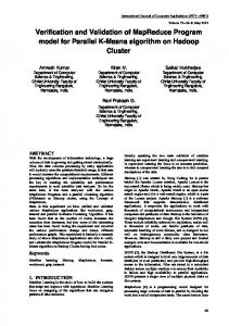
5.1 Improved Visualization Methods for External Validation The approach considered for visualization of external validation results for the GSM takes a number of key system or subsystem quantities and plots these as radial lines on a polar diagram [3, 4]. Values are normalized and shown as points on the radial axes. These points are then joined-up by straight lines to form a polygon, as shown in Figure 1. By plotting a polygon of model results and a polygon of measured results on the same polar diagram, an immediate indication of overall model validity is obtained. Moreover, aspects of the system that are represented more accurately than others are Volume 4, Number 1
JDMS vol 4 no 1 JAN 2007.indd 21
JDMS 21
3/12/2007 12:50:32 PM
Smith, Murray-Smith, and Hickman
c d
b
e
a
f
h
g
Figure 1. Example visualization of validation results: solid lines represent modeled results while broken lines represent corresponding measured results
immediately apparent, and this can highlight areas for further analysis. The polar representation is also an ideal way of displaying the results of sensitivity analysis [1]. The amount of distortion of the polygon resulting from some imposed change provides a visual representation of the relative sensitivities of quantities at system level or subsystem level. Further information may be added easily to this form of diagram. For example, the introduction of information relating to error bounds can indicate the operational limits, both of the system and the model. This approach to visualization of performance of models, although developed independently, has many features that are similar to the use of Kiviat diagrams [7], which are applied in software engineering for visualization of different metrics associated with software performance and computer hardware evaluation. The use of Kiviat diagrams has recently been extended into other fields such as business information [8] and is clearly applicable to problems in many areas where there is a need to depict relationships among multivariable data. Use of such diagrams in a modeling context still appears to be relatively novel, although the use of polygon figures as visualization tools in simulation model evaluation has recently been reported in the context of validation of dynamic simulation models in the paper industry [9]. Although the polygon displays can provide a valuable visual indicator of model performance, some
22 JDMS
means of quantifying the overall validity indicated by such diagrams is still necessary. Generally, the more similar the polygon shapes are for the system and the model the more valid the model is declared to be. The shape-based visualization lends itself to image processing methods for quantification, and a number of different approaches have been considered. Methods found to show promise included an approach to shape similarity assessment based on use of a multilayer perceptron (MLP) [10] and a morphological approach to non-linear image processing based on horizontal and vertical analysis of shapes [11]. In addition, approaches based on a fuzzy feature space similarity metric [12] and on a fuzzy syntactical pattern similarity metric [12] were found to give encouraging results. Consideration must be given to the order in which axes are chosen since altering the order will produce different shapes of polygon and the sensitivity of the tests will be affected. Three approaches have been identified in dealing with this issue. The first is to use prior knowledge and experience to establish the order. This is similar to the approach used for analysis of computer and software systems based on Kiviat diagrams. In that field of application it is common practice to group metrics by function on the diagram so that, for instance, metrics relating to memory usage are adjacent to each other. Such an approach makes all the measures within one category easily identifiable and, similarly, the ordering of axes in a polygon representing aspects of performance of a model could be grouped according to function. The second approach is to use information derived from error analysis and sensitivity analysis to identify critical data couplings and to base the order on those critical quantities. The third option is to consider all possible ordering arrangements and to adopt some indicator of the overall level of agreement based upon all of the available information. That is clearly the most time-consuming approach, but it provides a standard and objective method that is widely applicable and would involve calculating a quantitative measure of similarity for the polygon shapes for model and system results for every possible axis ordering arrangement. Simple statistical quantities, such as the average of all the calculated values of the similarity measures for all the possible ordering arrangements, could then be used to establish an overall quantitative indication of the level of agreement between model and system.
5.2 Illustrative Results Two sets of experiments were conducted to assess the relative merits of the different image processing
Volume 4, Number 1
JDMS vol 4 no 1 JAN 2007.indd 22
3/12/2007 12:50:33 PM
Verification and Validation Issues in a Generic Model of Electro-Optic Sensor Systems
methods in this context. The first set of tests used an artificially generated data set while the second used the results of the GSM together with simulated measurement data from a well-established computerbased model of a thermal imager system. This dual approach, based partly on artificial data, was adopted for two reasons. Firstly, in addition to experimental data from the real system, a straightforward data set was required so that validation issues could be explored and the various different metrics interpreted in a situation that was fully understood. Secondly, by controlling the artificial test data, behavioral characteristics and sensitivities could be set that would fully exercise the methods proposed. Figure 3. Shape comparisons: upper bounds of modeled and “measured” data for Test Set 1
5.2.1 Artificially Generated Data Two data sets were created, each involving five output quantities. These output quantities were chosen to provide appropriate measures of model and system performance for purposes of comparison. A modeled value was assigned to each quantity, and a set of five measurement values exhibiting different variations was also assigned to each quantity. This was equivalent to providing five sets of measured data from the real system. In addition, a relative importance weighting was given to each of the five parameters,
90 Test Set 1
Figure 4. Shape comparisons: lower bounds of modeled and “measured” data for Test Set 1
180
0
270
Figure 2. Polar plot of validation results for Test Set 1: five measurements were made of each of five measured quantities (solid lines indicate upper and lower bounds for the modeled case while broken lines indicate upper and lower bounds for measured quantities)
along with error bounds on the modeled values. The first data set was used for normalization. Figure 2 shows results for one data set (Data Set 1) plotted as a polar diagram. This polar plot has four separate polygons. Two of these polygons show the upper and lower bounds of the modeled case (solid lines), determined through error analysis and sensitivity analysis. The third and fourth polygons show the upper and lower extremes of the measurements (broken lines). The polygon plots of Figure 2 were converted to binary polygon images involving only the upper bounds of modeled and “measured” data, as shown in Figure 3. The validation methods must compare the upper bounds of the modeled results (i.e., the outer polygon) with the upper bounds of the “measured” results for both test sets. The same must be done with the lower bounds of the data. The latter shape comparisons are shown in Figure 4. Volume 4, Number 1
JDMS vol 4 no 1 JAN 2007.indd 23
JDMS 23
3/12/2007 12:50:33 PM
Smith, Murray-Smith, and Hickman
Each of the four image processing methods for polygon comparison, as outlined in section 5.1, was applied to the polygons of Figures 3 and 4. Results obtained using these image processing techniques are summarized in Table 1. The results in Table 1 include values for a second data set (Test Set 2) as well as for Test Set 1, to which Figures 2, 3, and 4 relate. The numerical results show that the MLP neural network performed well and ordered the shapes in agreement with ordering by eye. Values produced by this metric can range from 0 (totally dissimilar shapes) to 1 (identical shapes) but the range of values produced by these four tests was surprisingly large. The metrics based on the morphological horizontal-vertical root mean square (RMS) error are promising, although the table shows only results from the horizontal comparison. In order to fully determine the validity of a model, both horizontal and vertical analyses would be necessary and a final RMS error value formed for both would be required. However, if shapes appear to differ mainly in one direction, a limited morphological analysis may be justifiable. The fuzzy methods provide some interesting results. The approach based on the fuzzy feature space similarity metric was applied to all of the data in Test Set 1 and Test Set 2, using the standard deviation of the ‘measured’ results to define membership functions to compare with the modeled data. The modeled data did not have a distribution and so were set as crisp values. The fuzzy syntactic similarity metric also provided some promising results although there was little spread between the values calculated.
5.2.2 Thermal Imager Data A commercial package used for modeling of thermal imager performance (FLIR92) was chosen to provide a benchmark against which the GSM could be compared. The GSM was configured to represent a specific thermal imager system and a FLIR92 model was set up for the same thermal imager. Results from the two models were compared. The mathematical approaches of the FLIR92 and GSM models differ significantly in a number of important respects [3, 13], and the choice of the quantities used for the model comparisons took full account of those differences. Thermal imager systems are generally modeled as a series of modulation transfer functions (MTFs). Overall system performance may be expressed by a system transfer function or in terms of the minimum resolvable temperature difference (MRTD). A set of eight performance measures was chosen for testing purposes. This involved two subsystem MTFs (for the optics and for the A/D converter), one MTF for the eye (which is a component that is, of course, external to the thermal imager but can be included as a component of the model), two system MTFs for the vertical direction, and one for the horizontal direction. Three different MRTD values were also considered (for horizontal, vertical, and two-dimensional performance). Three different data sets were generated for testing purposes. One was produced using the GSM and the other two from FLIR92. One of the FLIR92 runs included the eye MTF and the other did not. This allowed two comparisons to be made by each validation technique to provide an indication of the sensitivity of each validation method to an element not represented within the GSM.
Table 1. Validation metric test results for artificially generated data. For each of the validation methods the upper bounds of the modeled results (i.e., the outer polygon in Figure 3 in the case of Data Set 1) were compared with the upper bounds of the “measured” results for both test data sets. The same was done with the lower bounds of the data (i.e., the polygons of Figure 4 in the case of Data Set 1).
Validation Method
Validation Parameter
Test Data Set 1 (Upper Bound)
Test Data Set 1 (Lower Bound)
Test Data Set 2 Test Data Set 2 (Upper Bound) (Lower Bound)
Nonlinear methods
RMS error of horizontal analysis of shapes
1.090
1.886
0.059
1.059
Neural networks
Multilayer perceptron (MLP) similarity value
0.839
0.976
0.442
0.123
1-dimensional similarity value
Fuzzy methods
24 JDMS
Syntactic similarity value
0.799 0.908
0.828 0.971
0.963
0.938
Volume 4, Number 1
JDMS vol 4 no 1 JAN 2007.indd 24
3/12/2007 12:50:33 PM
Verification and Validation Issues in a Generic Model of Electro-Optic Sensor Systems
Figure 5. Form of polar diagram for validation test cases for the thermal imager system
Polar diagrams of the form shown in Figure 5 were created for all three test cases. The polygons for test cases involving the GSM and FLIR 92 model without the eye MTF were very similar, whereas the third case for the FLIR92 model with the eye MTF produced a markedly different shape, as expected. As before, the polar diagram polygons were converted to binary images before running validation tests based on the MLP, nonlinear image processing and fuzzy methods, as outlined in section 5.2.1 . Table 2 summarizes the results of tests performed for these cases. These results also include metrics obtained using the cost function of equation (1) and
also using the TIC measure (equation (2)). It should be noted that the metrics of equations (1) and (2) only analyze results in terms of one quantity at a time, while the methods based on polygon images are intended for more complex situations involving several (or many) quantities. In order to compare the more standard validation metrics of equations (1) and (2) with the other methods, a cost value from equation (1) and a TIC value from equation (2) were calculated for each of the eight quantities of Figure 5 and an average taken to give the final value appearing in Table 2. Although the cost values found using equation (1) were disappointingly similar for the data sets with and without the eye MTF, much larger differences were found using some of the other techniques. For example, recalling that TIC has a value of zero for identical outputs and increases in value towards unity as differences increase, it can be seen that the GSM results in Table 2 compare well with the FLIR92 results for the case where the FLIR92 model does not include the eye MTF. However, the values of Table 2 for Theil’s Inequality Coefficient show that they do not compare well when the FLIR92 model does include the eye MTF. The value of TIC in the latter case is about 100 times larger than for the case where the GSM and FLIR92 results are both for the case without an eye MTF. This suggests that the inequality coefficient is a sensitive measure for validation purposes and that analysis based on this measure is potentially useful. Of the three methods that involve measures based on the polygon representation, the neural network and the fuzzy methods appear most promising. Although results obtained with the morphological approach to nonlinear image processing proved that this method can be applied to model validation problems, the processing time required was considerable.
Table 2. Validation test results for thermal imager data Metric Value Validation Method
Validation Parameter
GSM v FLIR92 Model Without Eye MTF
GSM v FLIR92 Model With Eye MTF
Cost function
Average cost
0.499
0.486
Theil’s inequality coefficient (TIC)
Average TIC value
0.003
0.272
Nonlinear methods
RMS error of horizontal count
0.015
0.154
Neural networks
Multilayer perceptron similarity value
0.999
0.533
1-dimensional similarity value
0.921
0.689
Syntactic similarity value
0.996
0.819
Fuzzy methods
Volume 4, Number 1
JDMS vol 4 no 1 JAN 2007.indd 25
JDMS 25
3/12/2007 12:50:33 PM
Smith, Murray-Smith, and Hickman
6. Discussion and Conclusions Limited conclusions can be drawn from the tests outlined here, but enough information has been gleaned to indicate the techniques are worthy of further research. Equally, the work described here allows a number of techniques to be dismissed. The main result from the work described is that the visualization method based on polygon shape comparisons is useful for the validation of complex models involving estimation of many key quantities. The advantage over the use of classical cost functions and measures such as Theil’s inequality coefficient is that the polygonal visualization method provides insight about the overall validity and about key sensitivities. Morphological processing and fuzzy statistical methods require further development to produce a robust metric that can be calculated quickly, although both these approaches show definite promise. The MLP neural network approach has been used to produce a validation metric that has been shown to be fast and incisive, although there is considerable scope for further work on optimization of such networks for validation purposes. Syntactic fuzzy pattern recognition has also been shown to give a useful metric. The value of any model depends greatly on the interpretation and analysis of its outputs. Within the framework of the GSM, a set of generic tools has been developed to allow the automated and easy interrogation of this computer-based description (optimization, sensitivity, and error analysis tools [1]). The development of a model validation tool provides a basis for investigating system model validity using traditional and novel metrics. Output result options for this tool already include tables of data for comparison, graphs, surfaces, and polar plots. The constraints imposed must include strict specification of input data so that true like-with-like comparisons may be made. Model results must also be available on file, with corresponding measured data for exactly the same sets of conditions. The tool thus provides a simple way of providing information about the validity of a model but requires intelligent use. Appropriate data must be compared, and validation metrics must be placed in the context of the intended application. Results must also be analyzed in conjunction with the information obtained from use of the sensitivity analysis and error analysis tools to allow a fuller understanding of the model limitations and its range of validity. Much scope remains for improving the validation tool, including more sophisticated data checking and the inclusion of further validation techniques. Nevertheless, in its
26 JDMS
present form, the validation tool is a valuable addition to the generic modeling framework. In terms of future developments, it is clear that assessment of different types of artificial neural network, the application of different morphological operators, and the extension of fuzzy analysis to n dimensions are all worthy of investigation.
7. References [1] Smith, M. I., D. J. Murray-Smith, and D. Hickman. “Mathematical and Computer Modeling of Electro-Optic Systems Using a Generic Modeling Environment,” Journal of Defense Modeling and Simulation 4 (1, 2007). [2] Murray-Smith, D. J. “Methods for the External Validation of Continuous System Simulation Models: A Review,” Mathematical and Computer Modeling of Dynamical Systems 4 (1, 1998) 5–31. [3] Smith, M. I. “The Design, Verification and Validation of a Generic Electro-optic Sensor Model for System Performance Evaluation,” Ph.D. Thesis, Department of Electronics and Electrical Engineering, University of Glasgow, 1999. [4] Smith, M. I., D. Hickman, and D. J. Murray-Smith. “Test, Verification and Validation Issues in Modeling a Generic Electro-Optic System,” Proceedings of the SPIE Annual Symposium, San Diego. Washington: SPIE Press, 1998. [5] Shakir, L. A. “The Complementary Use of Man-in-the-Loop and Closed-Loop Air Combat Models in Weapon System Effectiveness Studies,” Proceedings of the Second Test and Evaluation International Aerospace Forum, Royal Aeronautical Society, London, 1996. [6] Pace, D. K. “Verification, Validation and Accreditation.” In Applied Modeling and Simulation: An Integrated Approach to Development and Operation, edited by D. J. Cloud and L. B. Rainey, 369–409. New York: McGraw-Hill, 1998. [7] Kolence, K. and P. Kiviat. “Software Unit Profiles and Kiviat Figures, ACM SIGMETRICS,” Performance Evaluation Review 2 (3, 1973): 2–12. [8] Tegarden, D. P. “Business Information Visualization,” Communications of the Association for Information Sciences 1 (Paper 4, 1999): 1–34. Available from: http://cais.isworld.org/ articles/1-4/default.asp?view=html&x=66&y=4 [9] Kamml, G., H.-M. Voigt, and K. Neß. “Development of a Tool to Improve the Forecast Accuracy of Dynamic Simulation Models for the Paper Process.” In Cost Action E36, Modeling and Simulation in Pulp and Paper Industry, Proceedings of Model Validation Workshop, edited by J. Kappen and J. Manninen, VTT Symposium 238, October 6, 2005, VTT Research Centre of Finland, Espoo, Finland, 2005. [10] Rogers, S. K., and M. Kabrisky. An Introduction to Biological and Artificial Neural Networks for Pattern Recognition. Washgington: SPIE Optical Engineering Press, 1991. [11] Sinha, D., and C. R. Giardina. “Discrete Black and White Object Recognition via Morphological Functions,” IEEE Trans. On Pattern Analysis and Machine Intelligence 12 (3, 1990): 275–293. [12] Ross, T. J.Fuzzy Logic with Engineering Applications. McGrawHill, 1995. [13] Anon. FLIR92 Thermal Imaging Systems Performance Model, US Army Night Vision and Sensors Directorate, Doc. RG009993, 1993.
Volume 4, Number 1
JDMS vol 4 no 1 JAN 2007.indd 26
3/12/2007 12:50:33 PM
Verification and Validation Issues in a Generic Model of Electro-Optic Sensor Systems
Acknowledgement The authors are grateful to the reviewers for helpful suggestions that have led to significant improvements in this paper.
Author Biographies Dr. Moira Smith B.Eng., Ph.D., MRAeS, MIEE. Dr. Moira Smith is director of the technology consultancy company Waterfall Solutions Ltd., which specializes in image processing, algorithm and software development, and mathematical modeling, primarily for the defense industry. Heavily involved in the research and development of modeling and processing systems at an international level, Dr. Smith provides subject-matter expertise to the U.K. Ministry of Defence in this area and also leads training courses on data and image fusion. She has also authored papers on modeling and validation, chaired international conferences on EO systems modeling and processing, and is currently on SPIE’s security and surveillance organizing committee. Dr. Smith has a degree in avionics and a Ph.D. Prior to Waterfall Solutions she worked for Thales Optronics’ Algorithm Group developing EO processing algorithms and mathematical models for programs including Eurofighter and Fast Jet MWS. Dr. Smith also previously worked for Logica’s Aerospace and Defense Division developing real-time avionics software for helicopters and spacecraft systems.
Dr. Duncan Hickman B.Sc., M.Sc., Ph.D., M.Inst.P. Currently Chief Engineer for Waterfall Solutions Ltd., Dr. Hickman has responsibility for both design and engineering processes within the company, as well as business and technology strategy for future products. Dr. Hickman has considerable experience of major defense programs, including Eurofighter, TRACER, and FRES, and before joining Waterfall Solutions he was the Engineering Manager for the SeaWolf Mid-Life Update program. His expertise covers a wide range of technical areas, including electro-optical systems design and development, modeling, validation, processing algorithms and systems engineering, as well as group, project, and strategic management. Dr. Hickman holds a B.Sc., M.Sc. and Ph.D. in physics and is a Chartered Physicist. Before joining Waterfall Solutions he worked for BAE Systems Advanced Technology Centre, Oxford University, Matra Marconi Space Systems, Thales Optronics, and BAE Systems Insyte.
Dr. David Murray-Smith, B.Sc.(Eng.), M.Sc., Ph.D., FIEE. David Murray-Smith is an Emeritus Professor of the University of Glasgow. He is also an Adjunct Research Professor within the College of Engineering, Computer Science, and Construction Management at California State University, Chico. Until his retirement in 2005 he was Professor of Engineering Systems and Control in the Department of Electronics and Electrical Engineering at the University of Glasgow. Dr. Murray-Smith’s career began as a development engineer working on navigation systems with Ferranti Ltd., Edinburgh. His move to academic employment in the late 1960s led, over a period of about forty years, to active involvement in research in a number of different application areas including helicopter modeling and system identification, flight control, marine vehicle control, and to broader interests in simulation methodologies and model validation. David Murray-Smith has a B.Sc.(Eng.) in electrical engineering and also M.Sc. and Ph.D. degrees.
Volume 4, Number 1
JDMS vol 4 no 1 JAN 2007.indd 27
JDMS 27
3/12/2007 12:50:34 PM